Submitted:
03 July 2025
Posted:
04 July 2025
You are already at the latest version
Abstract
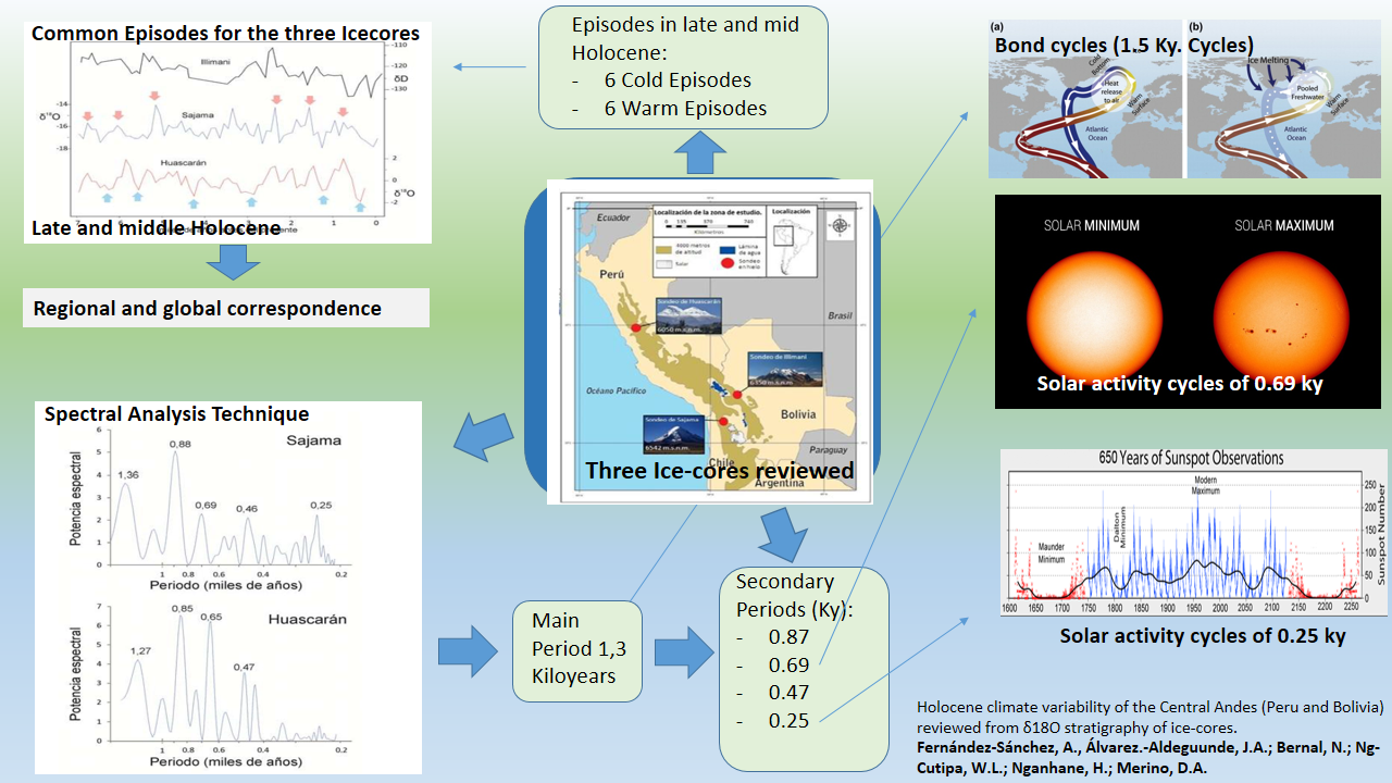
Glacial ice cores are evidence of past environmental conditions through gases and elements trapped inside the drilled material. As Central Andes in the southamerican region are very sensitive to climate changes, a great history of temperature and precipitation variability could be found related to massive Ice Caps. Available oxygen isotope data from glacial ice cores conducted over the last three decades in the Central Andes are reviewed to analyze climate variability over the past seven millennia, a period characterized globally by remarkable climatic stability. The analysis allowed for the identification of climate cycles ranging from secular to millennial in time. These cycles have periods of 1.3, 0.87, 0.67, 0.46, and 0.25 kiloyears (ky.). A series of regional thermal minima and maxima are also defined. This variability in the Andean climate during the mid- and late Holocene is interpreted as being strongly controlled by changes in solar activity, in particular, the forcing of "grand solar minima" is recognized. Likewise, less frequent climate changes could be correlated with Bond cycles and increased or decreased activity of the thermohaline circulation.
Keywords:
palaeoclimatology
; central andes
; past temperatures
; holocene
; stable isotopes
; δ18O stratigraphy
; spectral analysis
1. Introduction
Recent studies highlight the alarming rate at which Andean glaciers are retreating. Total amount includes a 35% faster (0.7 meters by year) retreat than the global average in the last decade [1]. Caro et al. [2] showed an increase of 12% in annual glacier melt for the Andean catchments driven by a 0.4oC shift in temperature and a 9% reduction in precipitation. This rapid loss underscores the urgency of understanding past climate patterns to predict future changes.
The Central Andes of South America have experienced significant climatic shifts during the Holocene period [3,4,5]. Sediment cores over lakes have shown aridity and precipitation changes in the Central Andes, suggesting climate patterns to have a major role on the centennial to millennial scales climate changes [6,7].
That millennial or centennial scale are also well documented in glacial ice cores drilled at high elevations, where no anthropic modifications have reached and representative regional weather conditions are presented. The trapped air bubbles and particulate matter within the ice cores could be a preserved record of past gas variability [8] or even anthropic activities [9]. The water content of each layer in the Ice-cores could have an amount of stable isotpoes (18O and Deuterium, D) representative of past precipitation and temperatures [10,11].
Thirty years of ice cores in the Central Andes have shed light on key aspects of regional climate evolution at the end of the Pleistocene and the Pleistocene-Holocene transition [12,13,14], as well as the last millennia (e.g., Eichler et al. [15]).
However, the results obtained for these time intervals have led to insufficient attention being paid to the more recent part of the record, particularly the interval between 7000 years BP and the last two millennia. This interval, characterized by relative climatic stability on a global scale, exhibits significant variability in the stable isotope records of Andean glacial ice.
By reviewing the stable isotope data series with new techniques, such as the Lomb-Scargle spectral analysis [16], hidden periodicities and variability of the so called “stable age” of the mid and late Holocene can be analyzed. Lomb Scargle periodogram has shown great results in the analysis of climate patterns [17,18], linking nowadays meteorological periodicities to regional atmospheric configurations.
The aim of this work is to review and re-analyze the palaeoclimate variability based on the available data. Specifically, this study reconstructs the palaeotemperatures of the last 7 ky. Before Present (BP). The variability is inferred from stable oxygen isotope stratigraphy in two ice cores in the Central Andes of Peru and Bolivia, primarily, and another complementary core with deuterium data.
1.1. Location of the Study Area
The analyzed ice cores are located in the Central Andes Mountains (Figure 1) of Peru and Bolivia. The Central Andes is a region of the Andean range that extends from Huancabamba (Peru) at 5oS to the Colorado River basin in the north of the province of Neuquén (Argentina), at 30oS. This section of the Andes contains some of the highest peaks in the range, including the Nevado Huascarán (the 5th highest peak in the Andes with 6757 m.) and Nevado Sajama (15th highest peak in the Andes with 6542 m.).
The Central Andes, as high mountains, are fully climate driven by the altitude modification of temperature, their tropical position and the Andean barrier to humidity fluxes from the Amazonia and Pacific Ocean. Precipitation (if solid or liquid) is related mainly to changes in latitude of the Inter Tropical Convergence Zone [19,20] and to El Niño Southern Oscillation pattern [21].
In this context, some Ice-cores samples were drilled between 1995 and 2003 in glacial ice caps. The Huascarán ice core, was drilled in the Cordillera Blanca of Peru (-9.269311, -77.497399, 6050 meters above sea level); while the Sajama core was drilled in the Central Volcanic Zone of Bolivia (-18.111102, -68.883429, 6542 m above sea level). The information is complemented by the stable hydrogen isotope series from the Illimani core that was drilled in the Cordillera Real of Bolivia (-16.630903, -67.791498, 6350 m above sea level).
2. Materials and Methods
The data from the Huascarán and Sajama cores were extracted from the NOAA (National Oceanic and Atmospheric Administration, USA) repository available at www.noaa.gov. These data correspond to the work of Thompson et al. [12,13]. The Illimani data are taken from Ramírez et al. [14]. The ratio of stable oxygen isotopes δ18O and hydrogen δD in glacial ice reflects the isotopic composition of precipitation over the duration of snowfall and, from this, palaeotemperatures can be estimated (e.g., Martín-Chivelet and Muñoz-García or Mc. Dermott [22,23]). The study of δ18O (and δD) stratigraphy allows us to analyze relative temperature variations in the intervals considered.
An important aspect is the resolution of the age models on which the time series of these surveys are based. Ice is very plastic, and layer counting (annual stratigraphy), whether visual or geochemical, can only be applied to the most recent levels (the last few centuries). Furthermore, 14C dating of organic remains trapped in the ice, and correlation with other better-dated records, allowed for a more refined dating of the late Pleistocene levels. However, most of the Holocene ice record (between 3,300 and 9,700 years BP in the case of Sajama and essentially the entire Holocene record in the case of Huascarán) was assigned an age according to a mathematical model. In the case of Illimani, the published age model is based on the correlation of major events (such as the Younger Dryas) with the Sajama survey [14]. The minimum error estimated for all age models is ±200 years. This significant limitation must be considered in intercomparisons between the series from the two surveys.
To simplify the visual and statistical comparison of the paleoclimate series, the proceeding was to eliminate long-term trends (“detrending”) superimposed on variability on a centennial or millennial scale. To achieve this, a linear fit was used in the case of Sajama and a second-order polynomial fit in Huascarán.
A spectral analysis of the Huascarán and Sajama time series was also performed to identify possible periodic elements in climate variability. For this purpose, the software PAST [24] was used, which works with the Lomb periodogram algorithm [16], which allows obtaining spectral diagrams from time series with non-equidistant values.
3. Results
The Sajama and Huascarán δ18O series (Figure 2), which also includes the δD record from the Illimani Ice core, show significant variability. The heaviest δ18O values correspond to higher temperatures and vice versa, allowing us to differentiate a series of alternating centennial-scale warming and cooling intervals in each series, as well as a series of episodes of relative minimum and maximum temperatures. A comparative analysis of the series allows us to identify patterns of common variability.
A tentative correlation of the local climatic maxima and minima is therefore established, assuming that they must have been essentially contemporaneous and that, therefore, the small lags between them can be attributed to the models’ error margins.
On the other hand, the results of the spectral analysis of the two surveys with the largest amount of data, represented in the spectral diagrams (Figure 3), show notable similarities, with spectral maxima around 1.3, 0.87, 0.67, 0.46, and 0.25 kiloyears, although the latter presents a very low level of significance in Huascarán.
4. Discussion
On the one hand, the identification of essentially contemporaneous climate minima and maxima (within the margins of error) in the three ice-cores analyzed, and on the other, the significant coincidences in cyclicity revealed by the spectral analysis, highlight the supraregional nature of the climate changes during the late and middle Holocene period.
To discuss the possible origin of these climate changes, the Andean records were compared with well-contrasted climate forcing and climate patterns time series. Specifically, with the total solar irradiance series [25] and with the relative activity series of the thermohaline circulation in the North Atlantic (records of glacioderived deposits in the North Atlantic, [26]).
Furthermore, glacial deposits derived from the North Atlantic show the existence of five maxima, all of which correspond well with the Andean climatic minima identified in this study (Figure 4). The glacial deposits in the North Atlantic are direct evidences of the thermohaline circulation. The thermohaline, also named as Atlantic Meridional Overturning Circulation (AMOC), is a key climate forcing for its role on energy distribution between hemispheres [27,28].
The AMOC velocity is very related to the meltwater flux that is naturally introduced in the North Atlantic area through Iceberg calving and terrain runoff [29]. These processes occur in cyclic “pulses” known as Heinrich Events, if the temporal scale ranges between 7 – 10 ky., or Dansgaard – Oeschger or Bond Cycles if it occurs each 1.5 ky. While Dansgaard-Oeschger events are related to the Pleistocene period, Bond Cycles are often referred to the Holocene [30]. Changes in the velocity (or a possible shut-off) can modify the interhemispheric energy balance, responding with global temperature variations in a short-term.
Slowing periods in the AMOC are closely related to rapid climate changes of abrupt cooling detected for the North Atlantic, but also for some other interconnected regions [28].
As tropical Atlantic Sea Surface Temperatures influence the large-scale atmospheric circulation, tropical eastern Pacific climate could be linked to AMOC [31]. Thermohaline circulation weakening is also a modulator of the Pacific El Niño pattern [32], which is also directly related to the Central Andes present temperatures [33] and Holocene palaeotemperatures [34].
The previous mentioned Bond cycles have been revealed present in different records sampled worldwide, showing possible Holocene climate teleconnection with North Atlantic. Renland Ice Cap core record (East central Greenland coast) showed climate variabilities in δ18O levels that were matched to a millennial-scale cycle in line with Bond Cycles [35].
Zielhofer et al. [36] found a noticeable lack of winter rain in the western Mediterranean during Early Holocene through δ18O records in Lake Sidi Ali (Morocco). The rain minima were coincident with Bond events while the opposite situation was found for the Late Holocene.
Records of the western European loess cores in Nussloch (Germany) matched also the variability of the North Atlantic, as they showed millennial scale changes in precipitation. This variability was pointed to connections with Bond Cycles [37].
In a local scale it is also possible to watch some coincidences between the Episodes here analyzed and other research. Some of the identified episodes, such as the Cold Episode V, matches cold conditions as marked by Weng et al. [38] in palynological analysis. This palynology also shows dry conditions coincident with the warm Episode IV during 5.0 Ky BP.
The above mentioned research in Nussloch [37] also identified a 4.2 ky potential anomaly that could match the Cold Episode IV (4.0 – 3.9 ka) registered in the Central Andes Ice-cores here revisited.
The cold Episode IV matches perfectly, as well, with glacier advances in the same study area. Cordillera Blanca could stand glacier readvances at 4 ky BP while the Nevado Sajama may have advances around the 4.4 ky BP [13]. The advances support the cold Episode IV, as some other episodes could be missing in the glacier record after geomorphological eroding of longest advances or during Little Ice Age.
Dry conditions [39] and a lack of glacier readvances are also coincident with a halt in climate variability between ~ 1.5 ky BP Cold Episode II and the warm Episode I during 0.4 – 0.7 Ky BP. Cold Episode I is coincident with the regional Little Ice Age so described for the Central Andes, and the researched glacier advances [40,41].
In parallel, the cycles recognized in the spectral analysis could be interpreted as connected to the global climate cycles related to these forcings. Specifically, the cycles defined by the longest periods (around 1.3 ky.) are close to the average length of Bond cycles, 1.5 ky. based on the recurrence of glacioderived deposits in the Atlantic and associated with changes in thermohaline circulation.
Links between North Atlantic Bond cycles and Aegean Sea climate fluctuactions (eastern Mediterranean) were also pointed through Spectral Analysis conducted over Ti/Al and Zr/Si records of a sediment core [42]. Among others, this research found a 1,200 year periodicity, closely related to the variability here found for the Central Andes.
Some authors have questioned the actual existence of Bond Cycles, identifying the origin of climate changes in several coinciding causes rather than just in the melt water origin [43]. As melt water pulses could be the key triggering factor for the abrupt changes in the Early Holocene, some other changes for the Late Holocene could be caused by a combination of mechanisms such as volcanic patterns, orbital insolation or Sun activity [44,45,46].
In this research, shorter-period cycles, of 0.69 and 0.25 ky, could tentatively be correlated with solar activity cycles of comparable duration [47,48].
Comparison of δ18O records from ice cores with forcing factor records (Figure 4) suggests a strong influence of solar activity on the three Central Andes ice cores. The major solar minima that mark the studied interval generally correspond well with episodes of minimum temperatures in the Central Andes.
Solar irradiation is the main driver for climatic circulation on Earth [25] and the paleoclimatic influence of solar activity has been widely proven [49,50].
Tropical Andes have been found to be very sensitive to even small changes in solar radiative forcing. Reduced solar activity in the Andes led to Little Ice Age period with a temperature decline of -3.2 +/-1.4oC at least for the venezuelan Andes [51,52]. Unfortunately, still there is a lack of information in the lower temporal scale to indicate the solar influence on past temperatures, as records are not accurate or have enough resolution [53].
In the Laguna Comercocha of the peruvian Andes, changes in sun activity have been linked to precipitation patterns through the modification of the South American Summer Monsoon intensity [54]. Therefore, directly because of a lack of radiative energy or indirectly because of climate patterns modification, solar forcing could be a key factor for the middle and late Holocene variability as revealed in the three reviewed ice-cores.
From all these findings, it can be deduced that the combined (and possibly interconnected) influence of solar activity and thermohaline circulation exert a strong control on climatic variations in the Southern Hemisphere and, in particular, to the Central Andes.
5. Conclusions
The main cold and warm episodes in the climate evolution of the central Andes over the last seven millennia have been identified using available data from glacial ice cores conducted in the area over the past few decades. The resolution achieved in this study is unprecedented in the Holocene palaeoclimatology of the region.
Spectral analysis techniques have shown to be a powerful tool for understanding the relationship between climate forcings and palaeclimatic variables.
As many other regions, Late and Middle Holocene variability of the Central Andes could be related to not only one single forcing but to more than one direct or indirect causes. A reviewing of stable isotopes from Ice-cores records from Nevado Sajama (Bolivia), Nevado Illimani (Bolivia) and Nevado Huascarán (Peru), could detect periodicities of 1,300 years in the palaeotemperatures. Also, shorter common cycles have been identified for 0.87, 0.69, 0.46 and 0.25 ky.
The longest periodicity identified, the 1.3 ky, suggests Bond Cycles events could be influencing palaeotemperatures in the Central Andes, while shorter cycles such as 0.69 and 0.25 ky. could be matched to solar activity.
Correlation analysis conducted over the ice records have also shown the relationship between minimum temperature episodes and minimum in sun activity. Also, warm and cold episodes have been identified as contemporary to close areas such other Andean regions, or to the Central Andes itself.
Among others, the climate variability is interpreted as related to major changes in solar activity during the Holocene, as well as long-term variations in thermohaline circulation (Bond cycles).
Author Contributions
Conceptualization, Nestor García Bernal; Data curation, Adrián Fernández-Sánchez; Formal analysis, Adrián Fernández-Sánchez; Investigation, Adrián Fernández-Sánchez; Methodology, Adrián Fernández-Sánchez and José Álvarez Aldegunde; Project administration, Helio Vasco Nganhane; Resources, Daniel Merino Panizo; Software, Adrián Fernández-Sánchez and José Álvarez Aldegunde; Supervision, Wai Ng-Cutipa, Helio Vasco Nganhane and Daniel Merino Panizo; Validation, José Álvarez Aldegunde; Visualization, Nestor García Bernal and Wai Ng-Cutipa; Writing – original draft, Adrián Fernández-Sánchez; Writing – review & editing, José Álvarez Aldegunde, Nestor García Bernal, Wai Ng-Cutipa, Helio Vasco Nganhane and Daniel Merino Panizo.
Funding
This research received no external funding
Data Availability Statement
links to publicly archived datasets analyzed https://www.ncei.noaa.gov/access/paleo-search/
Acknowledgments
Authors want to thank the editorial board and anonymous reviewers for their appreciated comments. The team would also like to thank KFA association for the precious support while researching.
Conflicts of Interest
The authors declare no conflicts of interest.
Conference Paper
This article is a revised and expanded version of a paper entitled “Revisión de la estratigrafía del δ 18 O en sondeos de hielo de glaciares de los Andes Centrales: Implicaciones para la variabilidad climática del Holoceno” which was presented at Geo-temas 16, 565-568, in 2016, Huelva, Spain.
Abbreviations
The following abbreviations are used in this manuscript:
| ITCZ | Inter Tropical Convergence Zone |
| ENSO | El Niño Southern Oscillation |
| N. | Nevado |
| BP | Before Present |
| Ky | Kiloyear (one thousand years) |
References
- A. Azoulay, “Message from Ms Audrey Azoulay, Director-General of UNESCO, on the occasion of World Day for Glaciers and World Water Day, 21 and 22 March 2025.” UNESCO Online, Mar. 22, 2025. Accessed: Apr. 20, 2025. [Online]. Available: https://unesdoc.unesco.org/ark:/48223/pf0000393199.
- A. Caro, T. Condom, A. Rabatel, N. Champollion, N. García, and F. Saavedra, “Hydrological Response of Andean Catchments to Recent Glacier Mass Loss,” May 23, 2023. [CrossRef]
- M. Grosjean, C. M. Santoro, L. G. Thompson, L. Núñez, and V. G. Standen, “Mid-Holocene climate and culture change in the South Central Andes,” in Climate Change and Cultural Dynamics, Elsevier, 2007, pp. 51–115. [CrossRef]
- S. Guédron et al., “Holocene variations in Lake Titicaca water level and their implications for sociopolitical developments in the central Andes,” Proc. Natl. Acad. Sci. U.S.A., vol. 120, no. 2, p. e2215882120, Jan. 2023. [CrossRef]
- H. Orellana, C. Latorre, J.-L. García, and F. Lambert, “Spatial analysis of paleoclimate variations based on proxy records in the south-central Andes (18°- 35° S) from 32 to 4 ka,” Quaternary Science Reviews, vol. 313, p. 108174, Aug. 2023. [CrossRef]
- J. A. Nunnery, S. C. Fritz, P. A. Baker, and W. Salenbien, “Lake-level variability in Salar de Coipasa, Bolivia during the past ∼40,000 yr,” Quat. res., vol. 91, no. 2, pp. 881–891, Mar. 2019. [CrossRef]
- J. N. Sae-Lim et al., “Biomarker evidence for arid intervals during the past ∼1,800 years in the central Andean highlands,” Earth and Planetary Science Letters, vol. 662, p. 119407, Jul. 2025. [CrossRef]
- J. Jouzel and V. Masson-Delmotte, “Deep ice cores: the need for going back in time,” Quaternary Science Reviews, vol. 29, no. 27–28, pp. 3683–3689, Dec. 2010. [CrossRef]
- A. Eichler, G. Gramlich, T. Kellerhals, L. Tobler, Th. Rehren, and M. Schwikowski, “Ice-core evidence of earliest extensive copper metallurgy in the Andes 2700 years ago,” Sci Rep, vol. 7, no. 1, p. 41855, Jan. 2017. [CrossRef]
- J. Jouzel et al., “Validity of the temperature reconstruction from water isotopes in ice cores,” J. Geophys. Res., vol. 102, no. C12, pp. 26471–26487, Nov. 1997. [CrossRef]
- S. J. Johnsen et al., “Oxygen isotope and palaeotemperature records from six Greenland ice-core stations: Camp Century, Dye-3, GRIP, GISP2, Renland and NorthGRIP,” J Quaternary Science, vol. 16, no. 4, pp. 299–307, May 2001. [CrossRef]
- L. G. Thompson et al., “A 25.000 Year Tropical Climate history from Bolivian Ice Cores,” Science, vol. 5395, no. 282, pp. 1858-1864., 1998.
- L. G. Thompson et al., “Late Glacial Stage and Holocene Tropical Ice Core Records from Huascarán, Peru,” Science, vol. 269, no. 5220, pp. 46–50, Jul. 1995. [CrossRef]
- E. Ramirez et al., “A new Andean deep ice core from Nevado Illimani (6350 m), Bolivia,” Earth and Planetary Science Letters, vol. 212, no. 3–4, pp. 337–350, Jul. 2003. [CrossRef]
- A. Eichler, G. Gramlich, T. Kellerhals, L. Tobler, and M. Schwikowski, “Pb pollution from leaded gasoline in South America in the context of a 2000-year metallurgical history,” Sci. Adv., vol. 1, no. 2, p. e1400196, Mar. 2015. [CrossRef]
- N. R. Lomb, “Least-squares frequency analysis of unequally spaced data,” Astrophys Space Sci, vol. 39, no. 2, pp. 447–462, Feb. 1976. [CrossRef]
- Y. Akdi and K. D. Ünlü, “Periodicity in precipitation and temperature for monthly data of Turkey,” Theor Appl Climatol, vol. 143, no. 3–4, pp. 957–968, Feb. 2021. [CrossRef]
- J. A. Álvarez Aldegunde, A. Fernández Sánchez, M. Saba, E. Quiñones, and J. Úbeda, “Analysis of PM2.5 and Meteorological Variables Using Enhanced Geospatial Techniques in Developing Countries: A Case Study of Cartagena de Indias City (Colombia),” Atmosphere, vol. 13, no. 506, p. 24, Mar. 2022. [CrossRef]
- T. Schneider, T. Bischoff, and G. H. Haug, “Migrations and dynamics of the intertropical convergence zone,” Nature, vol. 513, no. 7516, pp. 45–53, Sep. 2014. [CrossRef]
- S. Yuan et al., “The strength, position, and width changes of the intertropical convergence zone since the Last Glacial Maximum,” Proc. Natl. Acad. Sci. U.S.A., vol. 120, no. 47, p. e2217064120, Nov. 2023. [CrossRef]
- J. C. Sulca and R. P. D. Rocha, “Influence of the Coupling South Atlantic Convergence Zone-El Niño-Southern Oscillation (SACZ-ENSO) on the Projected Precipitation Changes over the Central Andes,” Climate, vol. 9, no. 5, p. 77, May 2021. [CrossRef]
- J. Martín-Chivelet and M. B. Muñoz García, “Estratigrafía de isótopos de oxígeno: reconstruyendo la variabilidad climática del pasado,” Enseñanza de las ciencias de la tierra: Revista de la Asociación Española para la Enseñanza de las Ciencias de la Tierra, vol. 23, no. 2, pp. 160–170, 2015.
- F. McDermott, “Palaeo-climate reconstruction from stable isotope variations in speleothems: a review,” Quaternary Science Reviews, vol. 23, no. 7–8, pp. 901–918, Apr. 2004. [CrossRef]
- O. Hammer, D. A. T. Harper, and P. D. Ryan, “PAST: Paleontological Statistics Software Package for Education and Data Analysis,” Palaeontologia Electronica, vol. 4, no. 1, p. 9, 2001.
- F. Steinhilber, J. Beer, and C. Fröhlich, “Total solar irradiance during the Holocene,” Geophysical Research Letters, vol. 36, no. 19, p. 2009GL040142, Oct. 2009. [CrossRef]
- G. Bond et al., “Persistent Solar Influence on North Atlantic Climate During the Holocene,” Science, vol. 294, no. 5549, pp. 2130–2136, Dec. 2001. [CrossRef]
- S. Manabe and R. J. Stouffer, “The role of thermohaline circulation in climate,” Tellus B, vol. 51, no. 1, pp. 91–109, Feb. 1999. [CrossRef]
- S. Rahmstorf, “Thermohaline ocean circulaion,” Encyclopedia of Quaternary Sciences, pp. 1–10, 2006.
- Z. Wang and L. A. Mysak, “Ice Sheet-Thermohaline Circulation Interactions in a Climate Model of Intermediate Complexity,” Journal of Oceanography, vol. 57, no. 4, pp. 481–494, 2001. [CrossRef]
- K. Sakai and W. R. Peltier, “A Dynamical Systems Model of the Dansgaard–Oeschger Oscillation and the Origin of the Bond Cycle,” J. Climate, vol. 12, no. 8, pp. 2238–2255, Aug. 1999. [CrossRef]
- A. Timmermann et al., “The Influence of a Weakening of the Atlantic Meridional Overturning Circulation on ENSO,” Journal of Climate, vol. 20, no. 19, pp. 4899–4919, Oct. 2007. [CrossRef]
- M. S. Williamson, M. Collins, S. S. Drijfhout, R. Kahana, J. V. Mecking, and T. M. Lenton, “Effect of AMOC collapse on ENSO in a high resolution general circulation model,” Clim Dyn, vol. 50, no. 7–8, pp. 2537–2552, Apr. 2018. [CrossRef]
- P. Good, N. Boers, C. A. Boulton, J. A. Lowe, and I. Richter, “How might a collapse in the Atlantic Meridional Overturning Circulation affect rainfall over tropical South America?,” Climate Resilience, vol. 1, no. 1, p. e26, Feb. 2022. [CrossRef]
- V. Jomelli et al., “In-phase millennial-scale glacier changes in the tropics and North Atlantic regions during the Holocene,” Nat Commun, vol. 13, no. 1, p. 1419, Mar. 2022. [CrossRef]
- A. G. Hughes et al., “High-frequency climate oscillations in the Holocene from a coastal-dome ice core in east central Greenland,” Feb. 24, 2020. [CrossRef]
- C. Zielhofer, A. Köhler, S. Mischke, A. Benkaddour, A. Mikdad, and W. J. Fletcher, “Western Mediterranean hydro-climatic consequences of Holocene ice-rafted debris (Bond) events,” Clim. Past, vol. 15, no. 2, pp. 463–475, Mar. 2019. [CrossRef]
- D. D. Rousseau et al., “Abrupt millennial climatic changes from Nussloch (Germany) Upper Weichselian eolian records during the Last Glaciation,” Quaternary Science Reviews, vol. 21, no. 14–15, pp. 1577–1582, Aug. 2002. [CrossRef]
- C. Weng, M. B. Bush, J. H. Curtis, A. L. Kolata, T. D. Dillehay, and M. W. Binford, “Deglaciation and Holocene climate change in the western Peruvian Andes,” Quat. res., vol. 66, no. 1, pp. 87–96, Jul. 2006. [CrossRef]
- O. Solomina, V. Jomelli, G. Kaser, A. Ames, B. Berger, and B. Pouyaud, “Lichenometry in the Cordillera Blanca, Peru: ‘Little Ice Age’ moraine chronology,” Global and Planetary Change, vol. 59, no. 1–4, pp. 225–235, Oct. 2007. [CrossRef]
- A. Rabatel, A. Machaca, B. Francou, and V. Jomelli, “Glacier recession on Cerro Charquini (16° S), Bolivia, since the maximum of the Little Ice Age (17th century),” J. Glaciol., vol. 52, no. 176, pp. 110–118, 2006. [CrossRef]
- V. Jomelli, D. Grancher, D. Brunstein, and O. Solomina, “Recalibration of the yellow Rhizocarpon growth curve in the Cordillera Blanca (Peru) and implications for LIA chronology,” Geomorphology, vol. 93, no. 3–4, pp. 201–212, Jan. 2008. [CrossRef]
- A. Noti, M. Geraga, L. J. Lourens, I. Iliopoulos, A. G. Vlachopoulos, and G. Papatheodorou, “Imprints of Holocene aridity variability in the Aegean Sea and interconnections with north-latitude areas,” The Holocene, vol. 34, no. 8, pp. 1036–1050, Aug. 2024. [CrossRef]
- H. Wanner and J. Butikofer, “Holocene bond cycles: Real or imaginary?,” Geografie, vol. 113, no. 4, pp. 338–350, 2008. [CrossRef]
- M. Schulz and A. Paul, “Holocene climate variability on centennial-to-millennial time scales: 1 Climate records from the North-Atlantic realm.,” in Climate development and history of the North Atlantic realm., In Wefer, G. et al., vol. 1, Berlin: Springer, 2002, pp. 41–54.
- M. Moros, J. T. Andrews, D. D. Eberl, and E. Jansen, “Holocene history of drift ice in the northern North Atlantic: Evidence for different spatial and temporal modes,” Paleoceanography, vol. 21, no. 2, p. 2005PA001214, Jun. 2006. [CrossRef]
- P. D. DITLEVSEN, K. K. ANDERSEN, and A. SVENSSON, “The DO-climate events are probably noise induced: statistical inverstigation of the claimed 1470 years cycle,” Climate of the Past, vol. 3, pp. 129–134, 2007.
- A. Asensio Ramos, “Extreme value theory and the solar cycle,” A&A, vol. 472, no. 1, pp. 293–298, Sep. 2007. [CrossRef]
- B. Komitov, “About the Possible Solar Nature of the ~200 yr (de Vries/Suess) and ~2000–2500 yr (Hallstadt) Cycles and Their Influences on the Earth’s Climate: The Role of Solar-Triggered Tectonic Processes in General ‘Sun–Climate’ Relationship,” Atmosphere, vol. 15, no. 5, p. 612, May 2024. [CrossRef]
- J.-M. Carozza et al., “The subfossil tree deposits from the Garonne Valley and their implications on Holocene alluvial plain dynamics,” Comptes Rendus. Géoscience, vol. 346, no. 1–2, pp. 20–27, Jan. 2014. [CrossRef]
- N. Brehm et al., “Eleven-year solar cycles over the last millennium revealed by radiocarbon in tree rings,” Nat. Geosci., vol. 14, no. 1, pp. 10–15, Jan. 2021. [CrossRef]
- P. Polissar, M. Abbott, A. Shemesh, A. Wolfe, and R. Bradley, “Holocene hydrologic balance of tropical South America from oxygen isotopes of lake sediment opal, Venezuelan Andes,” Earth and Planetary Science Letters, vol. 242, no. 3–4, pp. 375–389, Feb. 2006. [CrossRef]
- P. J. Polissar, M. B. Abbott, A. P. Wolfe, M. Bezada, V. Rull, and R. S. Bradley, “Solar modulation of Little Ice Age climate in the tropical Andes,” Proc. Natl. Acad. Sci. U.S.A., vol. 103, no. 24, pp. 8937–8942, Jun. 2006. [CrossRef]
- G. J. M. Versteegh, “Solar Forcing of Climate. 2: Evidence from the Past,” Space Sci Rev, vol. 120, no. 3–4, pp. 243–286, Oct. 2005. [CrossRef]
- K. Schittek, J. Wowrek, N. Käuffer, M. Reindel, and B. Mächtle, “Solar forcing as driver for late Holocene rainfall intensity in the Peruvian Andes,” Quaternary International, vol. 718, p. 109647, Feb. 2025. [CrossRef]
Figure 1.
Geographic location of the analyzed Ice-cores. Coordinates are written down in the main text.
Figure 1.
Geographic location of the analyzed Ice-cores. Coordinates are written down in the main text.
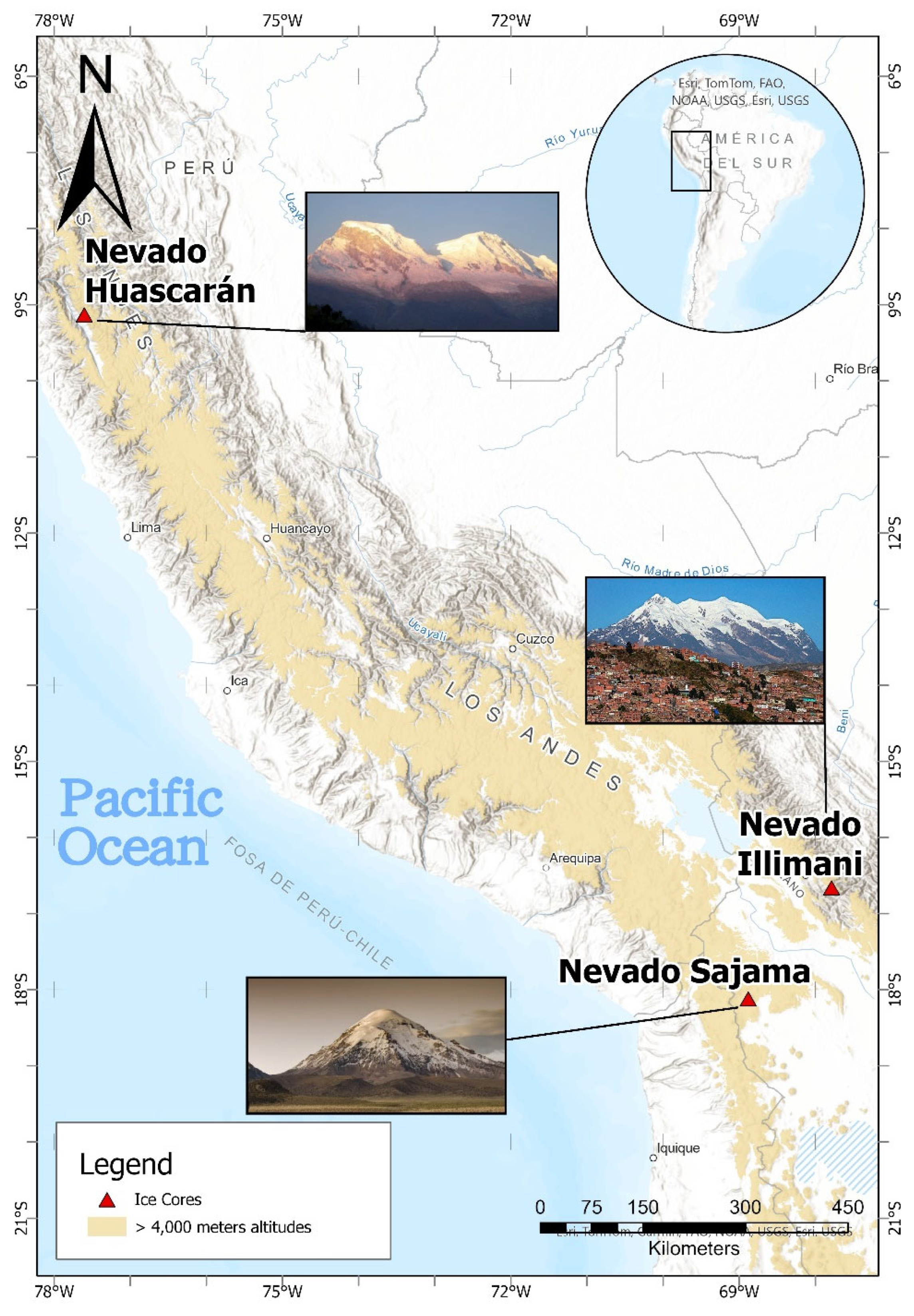
Figure 2.
Temporal data series of stable isotopes (δ18O and δD) contained in the Illimani, Sajama and Huascarán Ice-cores. Blue arrows indicate main cold episodes, while red arrows indicate maximum temperature episodes.
Figure 2.
Temporal data series of stable isotopes (δ18O and δD) contained in the Illimani, Sajama and Huascarán Ice-cores. Blue arrows indicate main cold episodes, while red arrows indicate maximum temperature episodes.
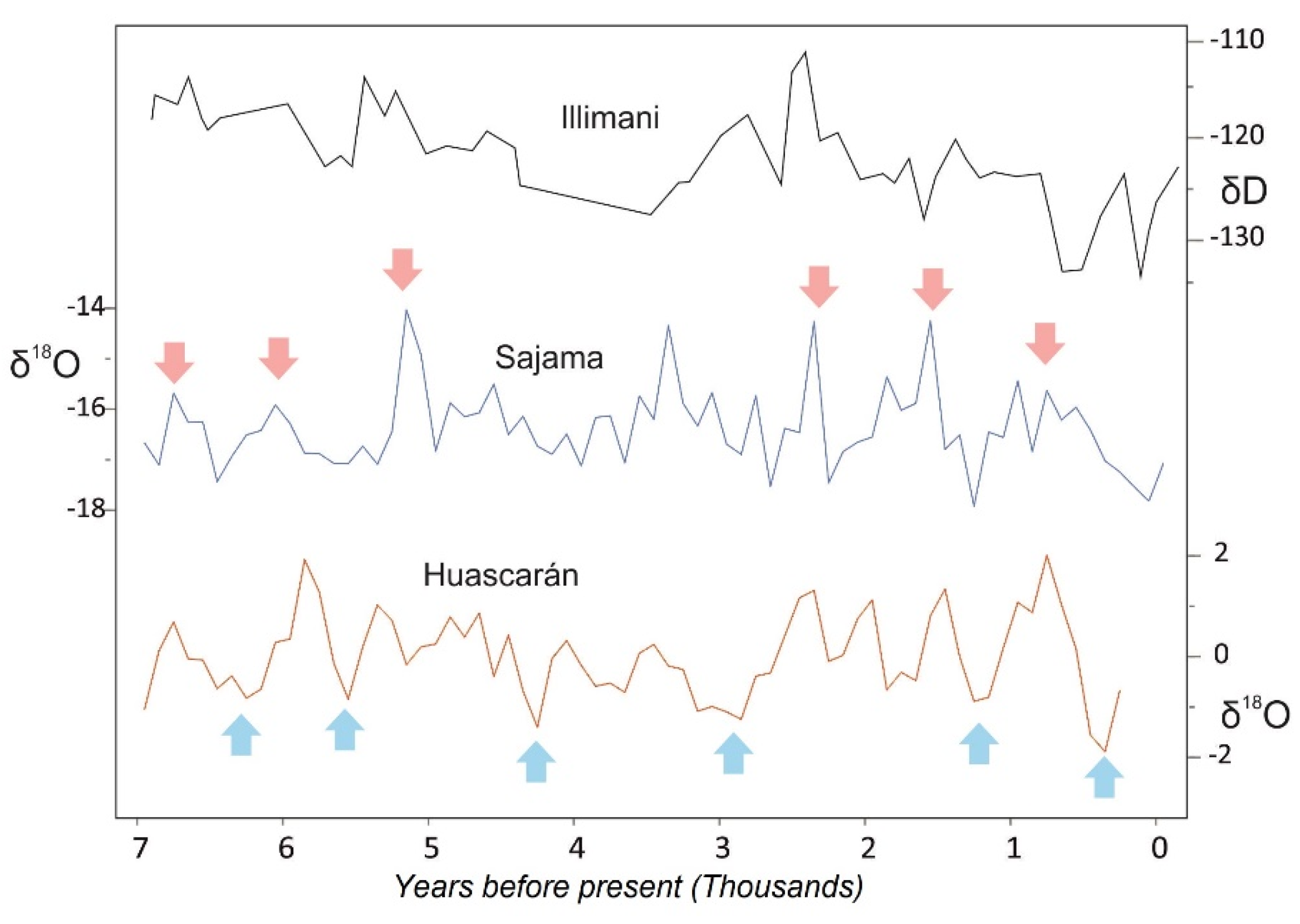
Figure 3.
Spectral diagrams of the oxygen isotopes data series derived from Andean ice-cores. The more significant spectral peaks are indicated in thousands of years.
Figure 3.
Spectral diagrams of the oxygen isotopes data series derived from Andean ice-cores. The more significant spectral peaks are indicated in thousands of years.
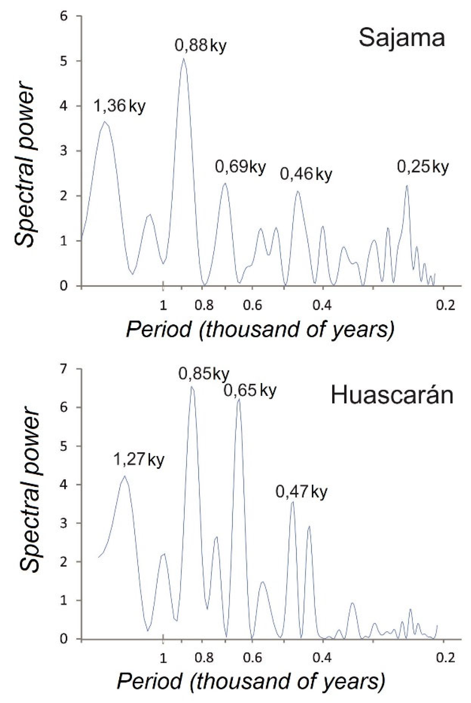
Figure 4.
Comparison of the stable isotopes data series from Sajama and Huascarán Ice-Cores with glacioderivated deposits of the Northern Atlantic (values expressed in percentaje of hematite grains; arrows indicated maximums corresponding to Iceberg massive entrances in the Atlantic, Bond et al. [26]), and with sun activity reconstruction (arrows indicating big solar minima; Steinhilber et al. [25]).
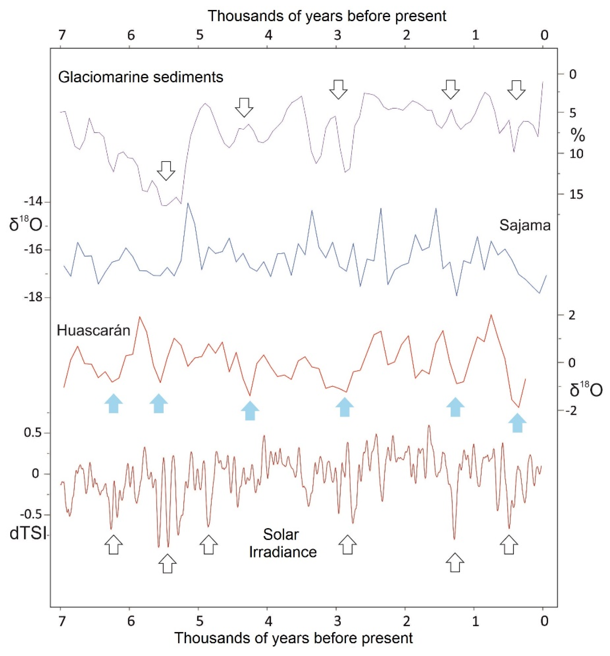

Table 1.
Warm episodes identifyied according to each of the Andean data series. Denomination of each episode is in the main header.
Table 1.
Warm episodes identifyied according to each of the Andean data series. Denomination of each episode is in the main header.
|
Core/ Warm Episode |
Episode VI |
Episode V |
Episode IV |
Episode III |
Episode II |
Episode I |
| N. Huascarán | 6.4 ky | 5.6 ky | 5.0 ky | 2.2 ky | 1.6 ky | 0.5 ky |
| N. Sajama | 6.6 ky | 5.9 ky | 5.0 ky | 2.4 ky | 1.5 ky | 0.7 ky |
| N. Illimani | 6.8 ky | 6.0 ky | 5.4 ky | 2.5 ky | 1.4 ky | 0.4 ky |
1 N. meaning “Nevado”, Spanish word for “high mountain”.
Table 2.
Cold episodes identified according to each of the Andean data series. Denomination of each episode is in the main header.
Table 2.
Cold episodes identified according to each of the Andean data series. Denomination of each episode is in the main header.
|
Core/ Cold Episode |
Episode VI |
Episode V |
Episode IV |
Episode III |
Episode II |
Episode I |
| N. Huascarán | 5.9 ky | 5.2 ky | 4.0 ky | 2.6 ky | 1.4 ky | 0.2 ky |
| N. Sajama | 6.4 ky | 5.5 ky | 3.9 ky | 2.6 ky | 1.2 ky | 0.1 ky |
| N. Illimani | 6.6 ky | 5.7 ky | 3.6 ky | 2.7 ky | - | 0.3 ky |
1 N. meaning “Nevado”, Spanish word for “high mountain”.
Disclaimer/Publisher’s Note: The statements, opinions and data contained in all publications are solely those of the individual author(s) and contributor(s) and not of MDPI and/or the editor(s). MDPI and/or the editor(s) disclaim responsibility for any injury to people or property resulting from any ideas, methods, instructions or products referred to in the content. |
© 2025 by the authors. Licensee MDPI, Basel, Switzerland. This article is an open access article distributed under the terms and conditions of the Creative Commons Attribution (CC BY) license (http://creativecommons.org/licenses/by/4.0/).
Copyright: This open access article is published under a Creative Commons CC BY 4.0 license, which permit the free download, distribution, and reuse, provided that the author and preprint are cited in any reuse.


