Submitted:
03 July 2025
Posted:
04 July 2025
You are already at the latest version
Abstract
This study aims to calibrate a detailed Finite Element (FE) model for simulating tensile tests on flat steel tensile coupons exhibiting a round stress strain behaviour. The model will be based on the widely utilized Johnson-Cook damage model, renowned for its accuracy in capturing material behavior under extreme loading conditions. Calibration will be achieved using experimental data obtained from flat dog bone specimens (tensile coupons) tested in controlled laboratory settings. The developed FE model will incorporate considerations for mechanical and geometric nonlin-earities, as well as the degradation of mechanical properties following necking. Through this research, we seek to enhance the fidelity and predictive capability of FE models by replicating the complex behavior of steel materials subjected to tensile loading.
Keywords:
finite element
; tensile test
; steel
; experimental
; damage
1. Introduction
Tensile testing is a fundamental practice in structural engineering, providing critical insights into the mechanical properties of materials, particularly steel. Understanding the behavior of steel under tensile loading conditions is essential for designing safe and efficient structures. Dog bone specimens, characterized by their standardized shape, play a crucial role in facilitating precise measurements during tensile tests. These specimens offer a consistent geometry that enables researchers to obtain reliable data for analysis.
In adherence to industry standards and guidelines like the ASTM E8/E8M [1], tension testing protocols are established, offering a framework for conducting experiments, including those involving dog bone specimens.
However, while experimental testing yields invaluable empirical data, its interpretation often requires a deeper comprehension of material behaviour under various loading scenarios. Herein lies the significance of Finite Element Method (FEM) modelling, which complements experimental observations with predictive numerical simulations. FEM modelling enables engineers to simulate the complex mechanical behaviour of steel dog bone specimens under diverse loading conditions, providing insights into stress distribution, deformation patterns, and failure mechanisms.
Crucially, the effectiveness of FEM modelling as a predictive tool hinge on the calibration of the numerical model to experimental data. By calibrating the model to accurately represent the physical behaviour observed in experimental tests, engineers ensure its validity and reliability for predictive purposes. This calibration process involves fine-tuning material properties, boundary conditions, and other model parameters to match the experimental results. Once calibrated, the validated FEM model serves as a powerful predictive tool, allowing engineers to explore a wide range of design scenarios and assess the structural performance of steel components with confidence.
Research endeavors have delved deep into understanding the mechanical behavior of steel dog bone specimens, utilizing both experimental approaches and numerical simulations. Studies by Luís P. Páez & José D. Moreira (2019) [2] and M. Melis et al. (2014) [3] have provided valuable insights into factors influencing tensile behavior, such as strain rate, temperature, and stress-strain relationships, through experimental and finite element analyses.
Moreover, investigations into the effects of external factors like heat treatment, alloying elements, and fatigue behavior have shed light on the intricate interplay between material properties and structural performance. Research conducted by A. Guo et al. (2018) [4], H. Wang et al. (2010) [5], and M. Wan et al. (2015) [6] has contributed significantly to this body of knowledge. Pei et al. (2021) [7] have shed light on the impact of sample geometry on material properties derived from uniaxial tensile tests.
Recent advancements in testing techniques, exemplified by studies from Karamoozian et al. (2019) [8], have incorporated digital image correlation (DIC) and acoustic emission (AE) analysis, further enhancing our ability to probe the mechanical properties of steel dog bone specimens.
Additionally, finite element simulation has emerged as a powerful tool in the analysis of tensile behavior. The incorporation of finite element simulation has emerged as a powerful tool in analysing the tensile behaviour of steel dog bone specimens under varying conditions. Studies such as those by Su et al. (2013) [10], Huang & Young (2014) [11], and Eom et al. (2014) [12] have provided valuable insights into various aspects, including plastic behaviour, constitutive relations, evaluation of damage models under tension.
These collective efforts represent a comprehensive state of the art in the field of tensile testing and finite element simulation of steel dog bone specimens. By integrating experimental findings with numerical simulations, researchers continue to advance our understanding of material behavior, informing the design and optimization of structures for enhanced safety and efficiency.
From the analysis of the state of art, it appears that there is a lack of sufficiently detailed studies enabling the full utilization of developed and proposed Finite Element (FE) models. Therefore, the objective of this work is to calibrate a detailed FE model based on the Johnson-Cook damage model, one of the most widely used theoretical models. This calibration will be achieved using experimental results from flat dog bone specimens (tensile coupons) tested in laboratory conditions. The model will account for mechanical and geometric nonlinearities, as well as the degradation of mechanical properties following necking.
2. Experimental Tests
Following two experimental campaigns conducted on Concrete Filled Steel Tubes (CFTs) with both square and circular sections [13,14], steel tensile coupons have been extracted to characterize the mechanical properties of the steel. The experimental campaign has been carried out at the Strength Laboratory of the University of Salerno.
2.1. Experimental Setup
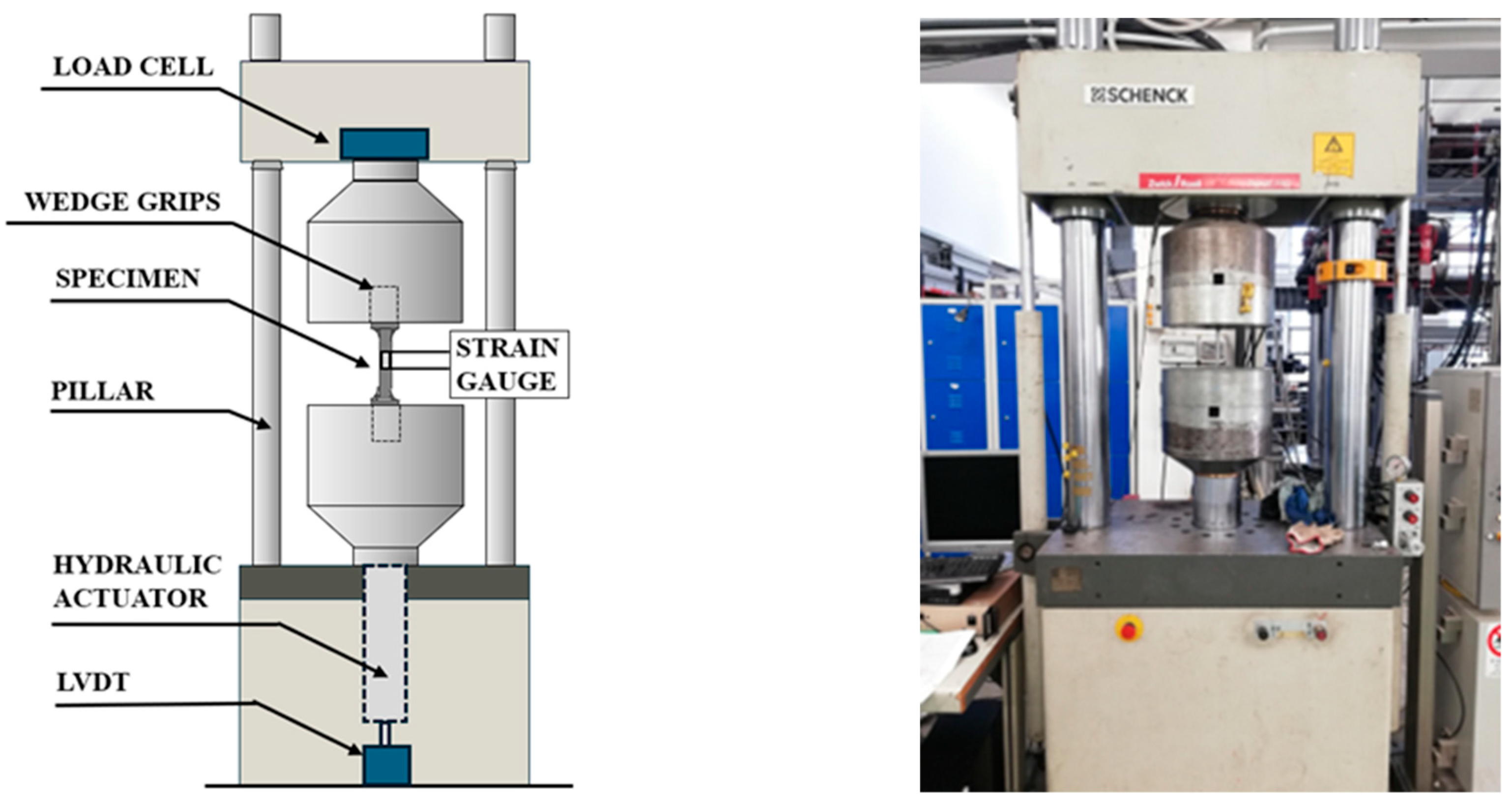
The mechanical properties of the steel tubes have been determined by means of standard tensile tests according to UNI EN ISO 6892-1-1 [15]. In particular, the tensile tests have been performed using a Schenck Hydropuls S56 testing machine with a maximum load of 630 kN and a piston stroke of ±125 mm. Tensile coupons have been extracted along the longitudinal direction of the plate elements constituting the cross-section. The monotonic tests have been conducted under displacement control according to Method A2 as described in [15]. The test speed is computed as a function of the calibrated length and the estimated strain rate :
Four intervals of speed, with the corresponding strain rate, are considered for predicting accurately the elastic and inelastic properties of the material.
The geometric dimensions (scheme in Figure 1) and the test speeds are reported in Table 1, where the tensile coupons derived from the square CFTs are labeled as S1-S8, while the ones derived from the circular CFTs as C1-C8.
The displacement and strain measurement instruments have been arranged as reported in the experimental setup scheme. In particular, strain gauges have been placed at the midspan section of the tested specimen in order to catch the strain evolution.
Figure 2.
Experimental setup scheme.
2.2. Results of the Experimental Tests
Two experimental tests have been performed for each configuration reported in Table 1. The mean values of the measured mechanical properties are reported in Table 2. In particular, the following parameters have been collected: the Young’s modulus , the conventional yield stress at a residual strain of 0.2% , the engineering maximum stress , the engineering strain corresponding to maximum stress and the ultimate strain . Moreover, the mean value of the specimen’s thickness is reported.
The stress-strain curves are reported in Figure 3, where it can be noted that the shape does not present any yielding plateau, but it is almost continuous being more similar to the one characteristic of high strength steel or aluminium.
3. Finite Element Modelling
This section discusses the Finite Element (FE) analysis conducted to simulate the experimental tests presented in Section 2. The analyses have been executed using the FE software Abaqus/CAE 2020, utilizing the Abaqus/explicit solver, known for its efficiency in parallel computing and its ability to manage damage evolution explicitly at each time step, through the state variables. The analysis aims to replicate the tensile behaviour of the tested specimens, considering material nonlinearities and damage behaviour [16,17].
3.1. Geometric Modelling, Boundary Conditions and Meshing Procedure
The geometric model has been reproduced through solid elements according to the dimensions reported in Table 1 and Table 2.
A meticulous partitioning procedure (Figure 4a) has been performed in order to apply a structured Hex-type mesh, known for its computational efficiency and ability to provide accurate results. In particular, three-dimensional, deformable and solid elements (C3D8R eight-node brick element with reduced integration type) have been adopted. Moreover, the Element Deletion feature has been activated, removing elements reaching the maximum allowable damage (), to simulate the failure bahaviour.
A mesh size averaging 3 mm has been chosen to strike a balance between precision and computational efficiency. Beginning with a mesh size of 10 mm, a sensitivity analysis gradually decreased to 1 mm. Below the average size of 5 mm, no notable alterations in the control parameters have been observed. A 3 mm size dimension has been selected to allow for a more accurate assessment of the failure behavior and to provide a finer evaluation of damage effects along the specimen's thickness (Figure 4b).
To impose the boundary conditions (BCs) and replicate the displacement history observed in the experimental test, coupling interactions between the grip surfaces and reference points (RP1, RP2) have been established (Figure 4c). A fixed support has been applied to RP2 while a displacement BC has been applied to RP1 (Figure 4d).
3.2. Modelling of the Mechanical Behaviour of Steel
In this section, the main mechanical properties of steel material are presented. The importance of accurately defining elastic, plastic, and damage behaviour is widely recognized, as it is essential for creating a precise model that can effectively simulate the structural response, including the progression up to failure. The elastic behaviour is described through the Young’s modulus and the conventional yield strength derived by the experimental tests performed on the tensile coupons, whose results are reported in Table 2.
Concerning plastic behavior, ABAQUS exploits the Von Mises yield criterion and an associated flow rule specifically tailored for ductile metals. The characterization of steel material behavior has been achieved through the results derived from experimental tests performed on the specimens, detailed in Section 2. Specifically, a kinematic hardening law has been incorporated, with parameters calibrated based on the true stress-true strain curves derived by the engineering ones reported in Figure 3.
The kinematic component of the hardening law, known as backstress has been defined as the sum of three backstress functions , represented in the stress-strain () plane, considering a reference system with the origin corresponding to the yielding condition point () (Figure 5a). Consequently, the kinematic backstress function can be expressed as follows:
where is the equivalent plastic strain; and are the parameters to be calibrated according to the experimental tests. The initial yield stress , has been set equal to the conventional yield stress . As an example, the calibrated backstress function for the C8 specimen is reported in Figure 5a. The hardening parameters employed for the FE simulation are listed in Table 3.
In the context of characterizing the material damage for steel, the Johnson-Cook damage model is one of the most employed to simulate the progressive degradation and failure of the material under cyclic loading conditions. This model incorporates a damage variable that evolves based on the equivalent plastic strain , equivalent fracture strain , and stress triaxiality , if strain rate and thermal effects are neglected. By defining the initiation of damage () and the failure condition (), the model effectively captures the material's response up to failure (Figure 6). According to this more complex theory, multiple failure modes could be activated.
However, in cases where uniaxial tensile stress states are considered, such as in tensile tests, the stress triaxiality remains constant until reaching the equivalent fracture strain and is set at 1/3. Therefore, for defining the initiation of damage, it becomes unnecessary to provide a complete Johnson-Cook curve. Instead, it suffices to define the stress triaxiality , set at 1/3, and the corresponding equivalent fracture strain to identify the onset of damage.
The equivalent fracture strain for each specimen has been defined according to the engineering maximum stress , reported in Table 2.
Furthermore, for determining the maximum damage (D=1), the displacement at failure is required. The defined FE model involves the activation of the damage function for a specific mesh element experiencing the defined pair. The mesh element will be deleted when reaching the equivalent plastic deformation corresponding to the displacement at failure , expressed as:
where is the equivalent failure strain and is the characteristic length of the mesh element, defined as the volume cubic root length. The failure strain can be obtained by extending the engineering stress-strain curves to the abscissa axis to derive the strain value at the intersection.
The values adopted for the displacement at failure and the characteristic lengths , are reported in Table 4. In particular, for the S1, S3, S4, S7, and S8 the values are not reported as the failure occurred in correspondence of the maximum stress.
4. Finite Element Simulation Results and Discussion
Based on the finite element modeling outlined in Section 3, this section presents and discusses the results of the simulation, starting with the comparison between experimental engineering stress-strain curves and those obtained through the Abaqus software (Figure 7 and Figure 8).
As described in Section 3, the behavior between the onset of damage (D=0) and failure (D=1) has been described as linear. This assumption is evident from the analysis of the figures. Such simplification allows for an accurate capture of stress and strain at failure, albeit losing some details at the elbow of the curve. It is worth noting that some tests failed before the onset of degrading behavior (S1, S3, S7, S8). In such cases, for the simulation, it is possible to impose a failure point close to the maximum stress or continue with a trend derived experimentally from tests with similar characteristics. The fitting is testified by a maximum percentage error in the definition of the maximum stress of 3% and the failure stress of 5%. In addition to showing good fitting, the FEM simulation has respected the various phases encountered by the tensile coupon during the tensile test. In particular, it is possible to observe: 1) elastic phase (Figure 9a); 2) maximum stress and initial necking (Figure 9b); 3) degradation of mechanical properties (Figure 9c); 4) failure of the specimen (Figure 9d).
5. Conclusions
The study herein presented delves into the calibration of a detailed Finite Element (FE) model aimed at simulating tensile tests on flat steel tensile coupons. Tensile testing stands as a cornerstone in structural engineering, offering critical insights into the mechanical properties of materials, and particularly steel. The calibrated FE model, based on a damage model for ductile metals, seeks to refine a predictive numerical simulation model to be applied for other purposes. The main findings of the study are reported in bullets:
- The FE simulation, calibrated based on experimental data, effectively captures the mechanical behaviour of steel under tensile loading conditions.
- The linear assumption between the onset of damage and failure allows for accurate prediction of stress and strain at failure, with minor loss of detail.
- The simulation results closely match the experimental observations, with a maximum percentage error within acceptable limits (3-5%).
- The FEM model accurately replicates the various phases of the tensile test, demonstrating its reliability and predictive capability.
- These findings underscore the importance of detailed calibration and validation of FE models for accurately simulating material behaviour and structural response.
Author Contributions
Conceptualization, V.P., E.N and R.M.; Methodology, P.T, E.N., V.P and R. M.; Software, E.N. and P. T.; Validation, E.N., and P.T.; Formal analysis, E.N and P.T.; Investigation, E.N. and P.T.; Writing – original draft, E.N. and P.T.; Writing – review & editing, R.M. and V.P.; Supervision, V.P. and R.M.
Funding
This research received no external funding.
Conflicts of Interest
The authors declare no conflicts of interest.
References
- ASTM International, Standard Test Methods for Tension Testing of Metallic Materials, ASTM E8/E8M-22, 2022, Volume 03.01. [CrossRef]
- Páez, L.P.; Moreira, J.D. Tensile behavior of structural steel dog-bone specimens: Experimental and numerical analysis. Thin-Walled Struct. 2019, 144, 106403.
- Melis, M. Experimental and numerical study on the tensile behavior of dog-bone specimens made of steel grade S1100. In Procedia Engineering; [Editors], Eds.; Elsevier: Amsterdam, The Netherlands, 2014; Volume 88, pp. 85–91.
- Guo, A. Effect of heat treatment on the microstructure and mechanical properties of 12CrNi2 steel dog bone specimens. J. Iron Steel Res. Int. 2018, 25(11), 1195–1201.
- Wang, H. Tensile properties and microstructure of a high strength steel under different alloying element conditions. Mater. Sci. Eng. A 2010, 527(9-10), 2516–2523.
- Wan, M. Low cycle fatigue behavior of Cr–Mo–V–Ni–Al steel at room and elevated temperatures. Mater. Sci. Eng. 2015, 648, 329–336.
- Pei, M., Zou, D., Gao, Y., Zhang, J., Huang, P., Wang, J., Huang, J., Li, Z., & Chen, Y. The influence of sample geometry and size on porcine aortic material properties from uniaxial tensile tests using custom-designed tissue cutters, clamps and molds. PLoS One, 2021, 16(2), e0244390. [CrossRef]
- Karamoozian, S.; Experimental investigation on the effect of artificial aging treatment on the mechanical properties of AA7150 aluminum alloy. Mater. Sci. Eng. 2019, 742, 309–317.
- Joun, M., Choi, I., Eom, J., & Lee, M. Finite element analysis of tensile testing with emphasis on necking. Comp. Mat. Sci., 2007, 41, 63-69. [CrossRef]
- Su, J., Guo, W., Meng, W., & Wang, J. Plastic behavior and constitutive relations of DH-36 steel over a wide spectrum of strain rates and temperatures under tension. Mech. Mater., 2013, 65, 76-87. [CrossRef]
- Huang, Y., & Young, B. The Art of Coupon Tests. J. Constr. Steel Res., 2014, 96, 159-175. [CrossRef]
- Eom, J., Kim, M., Lee, S., Ryu, H., & Joun, M. Evaluation of damage models by finite element prediction of fracture in cylindrical tensile test. J. Nanosci. Nanotechnol., 2014, 14(10), 8019-8023. [CrossRef]
- Montuori R., Nastri E., Piluso V., Pisapia A., Todisco P. Experimental study and finite element damage modelling of concrete-filled structural elements under pure bending (2025) Structures, 74, art. no. 108574. [CrossRef]
- Montuori, R., Nastri, E., Piluso, V., Todisco, P., “Experimental and analytical study on the behaviour of circular concrete filled steel tubes in cyclic bending”, (2024) Engineering Structures, Volume 304, 117610, ttps://doi.org/10.1016/j.engstruct.2024.117610.
- UNI-EN-ISO 6892-1: “Metallic materials – Tensile testing – Part 1: Method of test at room temperature”, European Standard, 2020.
- Ribeiro J., Santiago A., Rigueiro C. “Damage model calibration and application for S355 steel” (2016) Procedia Structural Integrity, 2, pp. 656 - 663. [CrossRef]
- Montuori R., Nastri E., Piluso V., Todisco P. Finite element analysis of concrete filled steel tubes subjected to cyclic bending (2024) Engineering Structures, 314, art. no. 118364. [CrossRef]
Figure 1.
Tensile coupon dimensions scheme (a) and example of tested specimens (b).
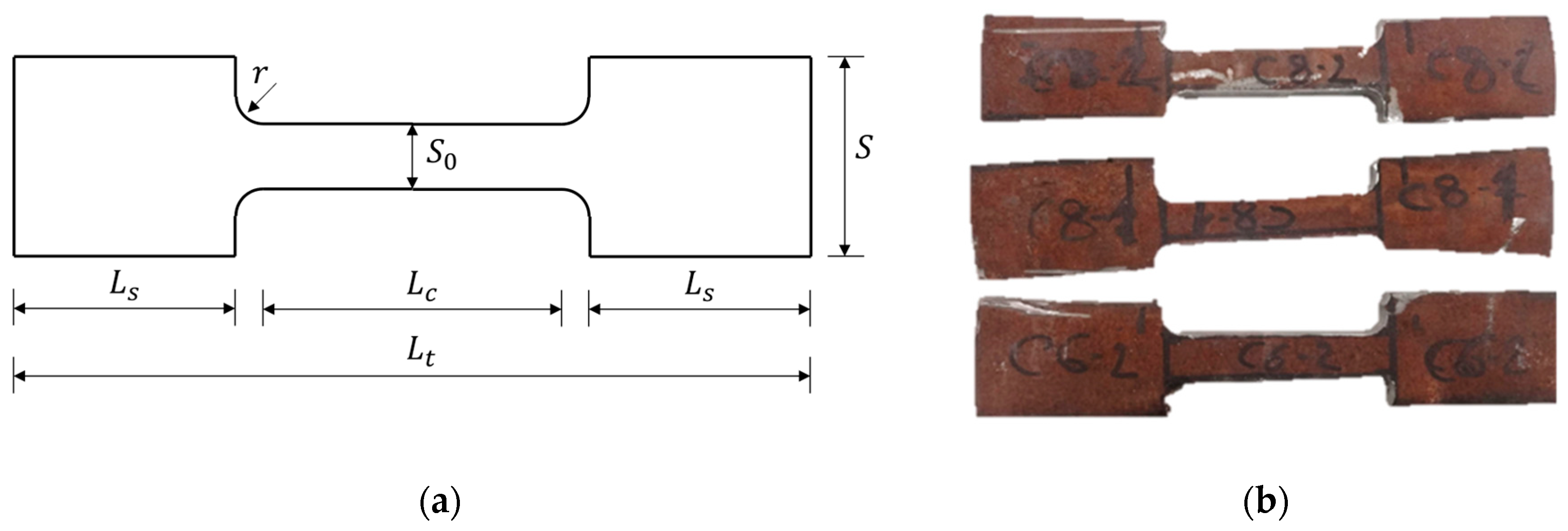
Figure 3.
Results of the experimental tests: S1-S8 (a); C1-C8 (b).
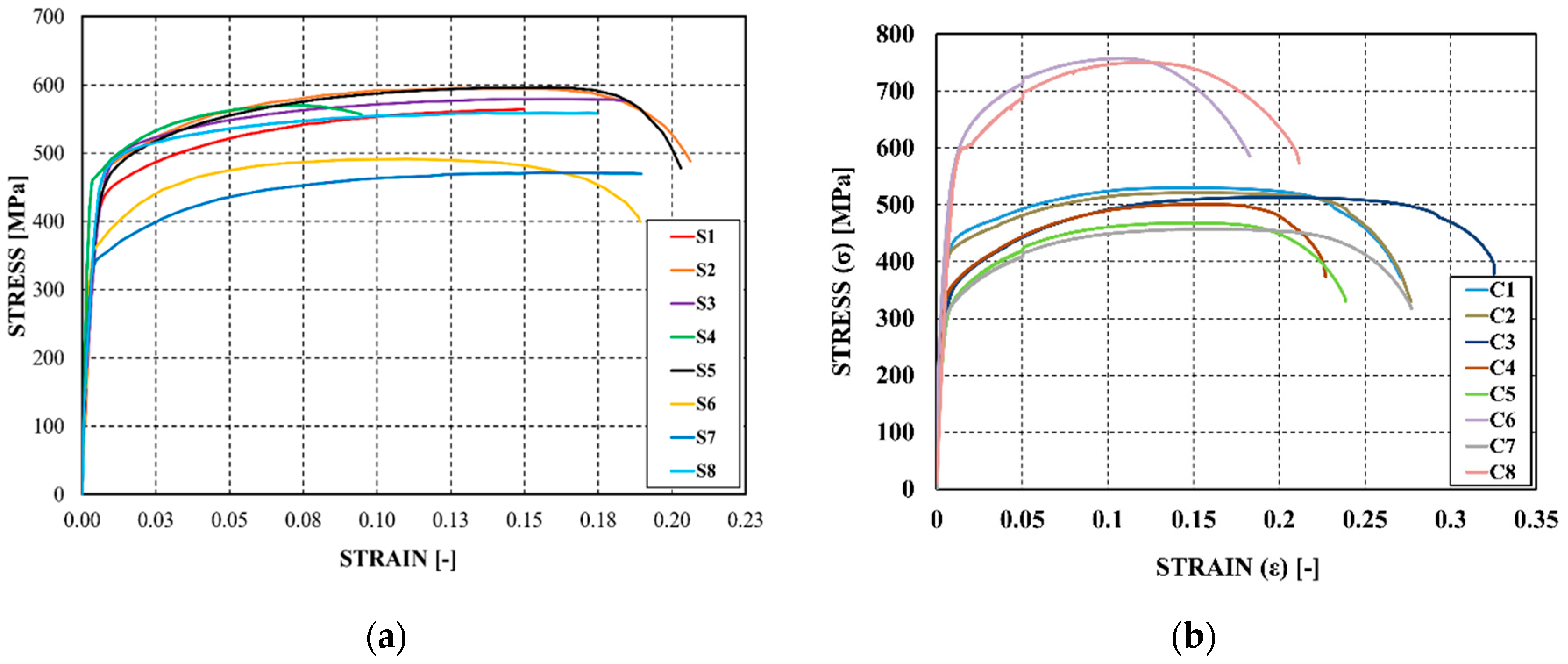
Figure 4.
Partitioning procedure (a); interactions (b); boundary conditions (c); mesh pattern (d).
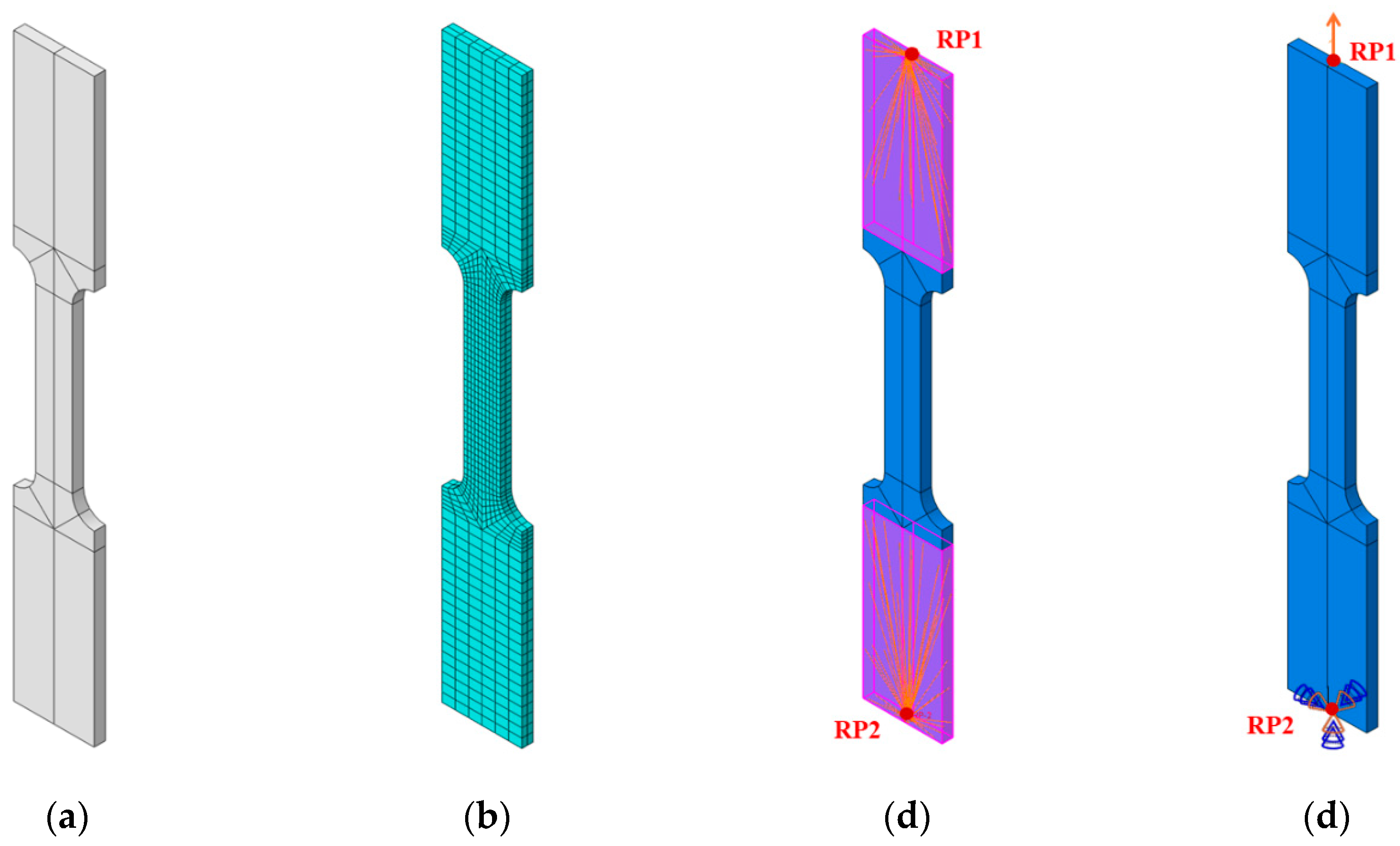
Figure 5.
Backstress reference system (a); Backstress function calibration - C8 specimen (b).

Figure 6.
Damage model for ductile metals.
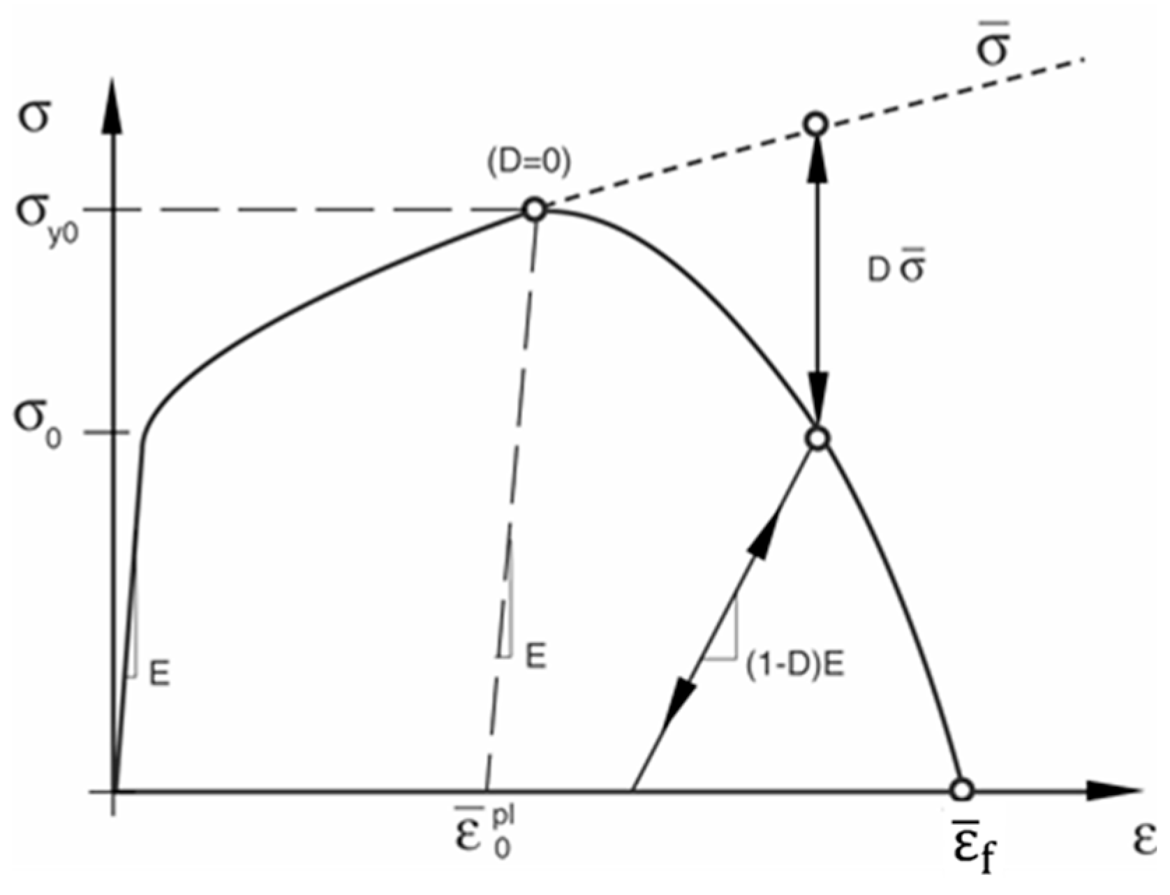
Figure 7.
Comparison between experimental and FE simulation Stress-strain curves (S1-S8).
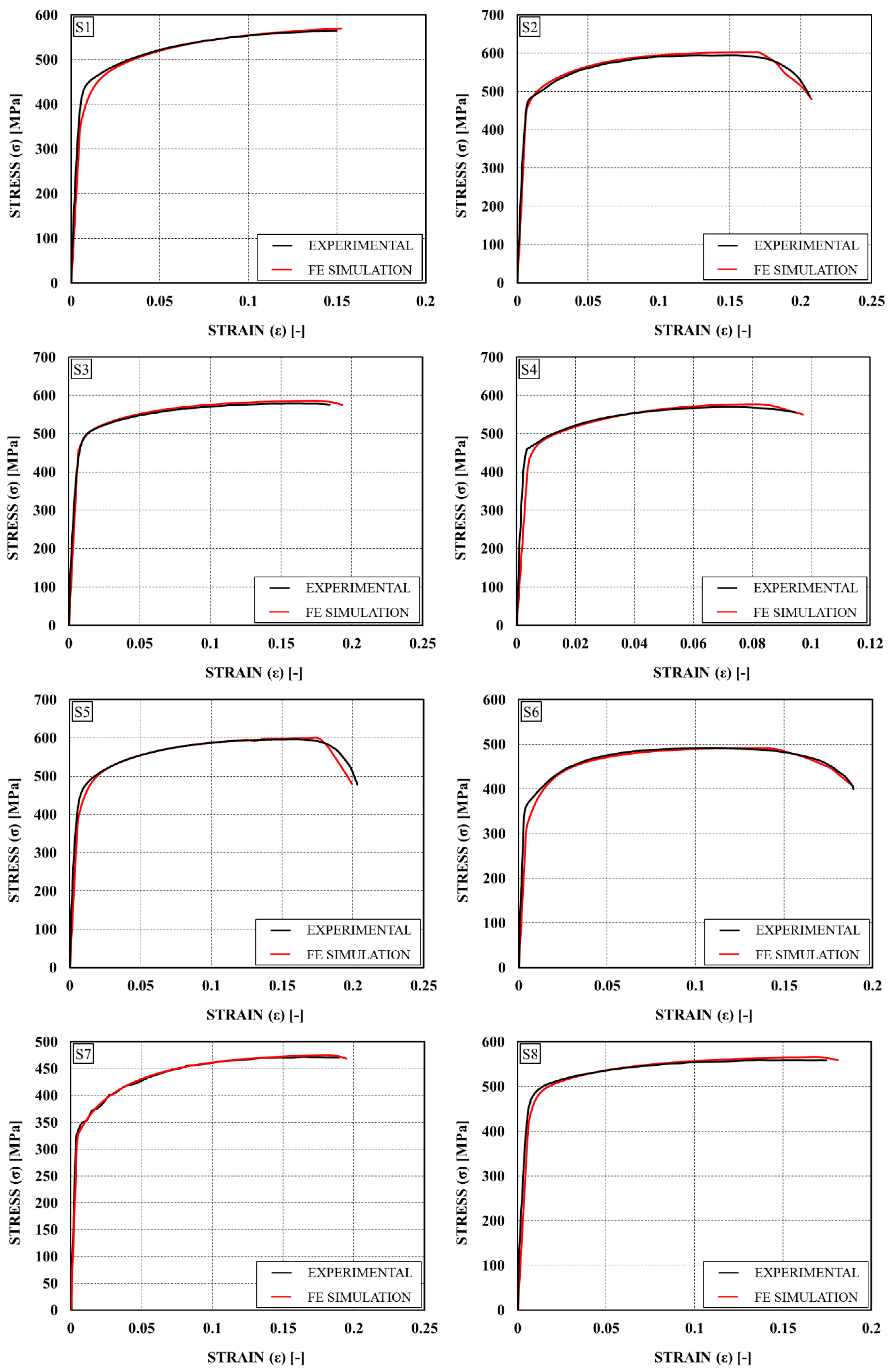
Figure 8.
Comparison between experimental and FE simulation Stress-strain curves (C1-C8).
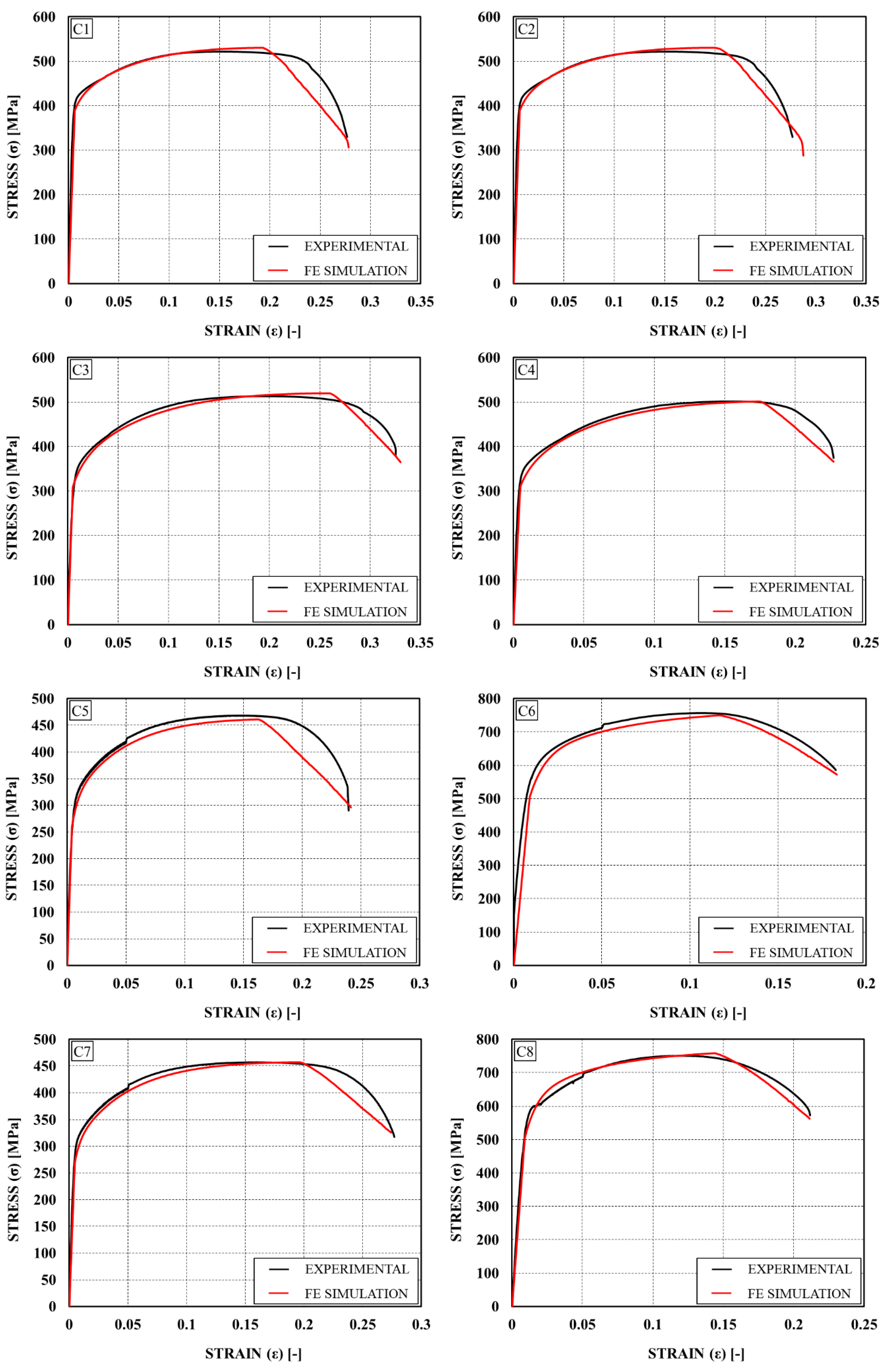
Figure 9.
Elastic phase (a); maximum stress (b); degradation of mechanical properties (c); failure (d).
Figure 9.
Elastic phase (a); maximum stress (b); degradation of mechanical properties (c); failure (d).
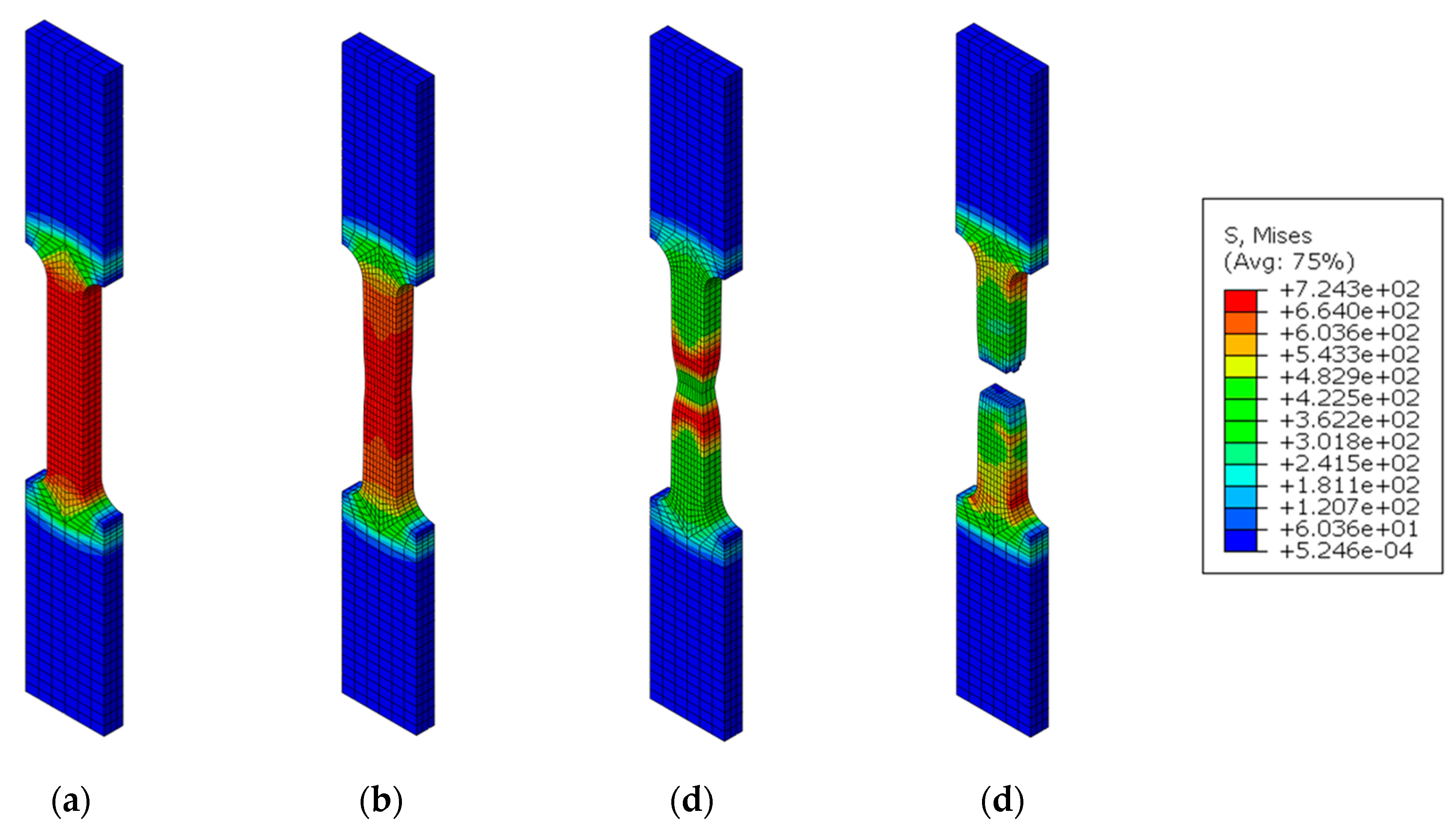

Table 1.
Geometric configuration and test speeds of the tested specimens.
| Label |
[mm] |
[mm] |
[mm] |
[mm] |
[mm] |
[mm] |
[mm/s] |
[mm/s] |
[mm/s] |
[mm/s] |
|---|---|---|---|---|---|---|---|---|---|---|
| S1, S3, S5, S8 | 39 | 90 | 160 | 100 | 360 | 15 | 0.0112 | 0.040 | 0.32 | 1.072 |
| S2, S4, S6, S7 | 30 | 90 | 160 | 100 | 360 | 15 | 0.0112 | 0.040 | 0.32 | 1.072 |
| C1-C8 | 20 | 44 | 90 | 93 | 300 | 12 | 0.0063 | 0.0225 | 0.18 | 0.603 |
Table 2.
Mean values of the measured mechanical properties and thickness of the specimens.
| Label |
[mm] |
[MPa] |
[MPa] |
[MPa |
[-] |
[-] |
|---|---|---|---|---|---|---|
| S1 | 7.70 | 428.34 | 564.28 | 564.28 | 0.15 | 0.15 |
| S2 | 6.10 | 493.31 | 595.08 | 488.19 | 0.12 | 0.21 |
| S3 | 7.70 | 462.28 | 579.35 | 576.80 | 0.16 | 0.16 |
| S4 | 6.10 | 459.93 | 570.49 | 556.89 | 0.07 | 0.09 |
| S5 | 7.80 | 447.87 | 596.25 | 477.98 | 0.16 | 0.20 |
| S6 | 4.90 | 359.80 | 491.25 | 399.24 | 0.11 | 0.19 |
| S7 | 4.90 | 342.63 | 471.58 | 469.44 | 0.15 | 0.19 |
| S8 | 7.80 | 428.34 | 564.28 | 558.49 | 0.15 | 0.17 |
| C1 | 9.50 | 375.05 | 500.94 | 331.99 | 0.16 | 0.27 |
| C2 | 9.50 | 387.51 | 510.17 | 374.93 | 0.14 | 0.26 |
| C3 | 6.40 | 357.54 | 508.46 | 335.33 | 0.18 | 0.30 |
| C4 | 6.40 | 352.60 | 495.82 | 293.51 | 0.13 | 0.22 |
| C5 | 6.10 | 252.61 | 458.40 | 564.44 | 0.17 | 0.26 |
| C6 | 10.40 | 522.53 | 746.00 | 296.15 | 0.10 | 0.16 |
| C7 | 6.20 | 267.48 | 440.74 | 535.77 | 0.15 | 0.21 |
| C8 | 10.60 | 542.49 | 732.47 | 331.99 | 0.12 | 0.20 |
Table 3.
Kinematic hardening parameters.
| Label |
[-] |
[-] |
[-] |
[-] |
[-] |
[-] |
|---|---|---|---|---|---|---|
| S1 | 22000 | 250 | 2600 | 28 | 920 | 1 |
| S2 | 10000 | 250 | 2500 | 25 | 800 | 1 |
| S3 | 11500 | 250 | 1750 | 25 | 800 | 1 |
| S4 | 15000 | 280 | 3500 | 28 | 450 | 1 |
| S5 | 18000 | 200 | 2400 | 21 | 800 | 1 |
| S6 | 16000 | 200 | 2850 | 28 | 580 | 1 |
| S7 | 5800 | 200 | 2600 | 22 | 590 | 1 |
| S8 | 1500 | 250 | 2050 | 28 | 750 | 1 |
| C1 | 3400 | 150 | 2200 | 20 | 550 | 1 |
| C2 | 3500 | 150 | 2000 | 18 | 650 | 1 |
| C3 | 4700 | 100 | 2250 | 15 | 700 | 1 |
| C4 | 5100 | 150 | 3200 | 20 | 600 | 1 |
| C5 | 10500 | 150 | 3700 | 20 | 500 | 1 |
| C6 | 21000 | 200 | 3200 | 25 | 1150 | 1 |
| C7 | 10000 | 210 | 3600 | 25 | 650 | 1 |
| C8 | 12000 | 200 | 2600 | 25 | 1050 | 1 |
Table 4.
Displacement at failure and characteristic length values.
| Label |
[mm] |
[mm] |
|---|---|---|
| S1 | - | 2.49 |
| S2 | 0.95 | 2.30 |
| S3 | - | 2.49 |
| S4 | - | 2.30 |
| S5 | 0.90 | 2.50 |
| S6 | 0.65 | 2.14 |
| S7 | - | 2.14 |
| S8 | - | 2.50 |
| C1 | 0.95 | 2.67 |
| C2 | 0.95 | 2.67 |
| C3 | 1.15 | 2.35 |
| C4 | 1.00 | 2.35 |
| C5 | 0.92 | 2.30 |
| C6 | 1.46 | 3.46 |
| C7 | 1.00 | 2.31 |
| C8 | 1.77 | 3.53 |
Disclaimer/Publisher’s Note: The statements, opinions and data contained in all publications are solely those of the individual author(s) and contributor(s) and not of MDPI and/or the editor(s). MDPI and/or the editor(s) disclaim responsibility for any injury to people or property resulting from any ideas, methods, instructions or products referred to in the content. |
© 2025 by the authors. Licensee MDPI, Basel, Switzerland. This article is an open access article distributed under the terms and conditions of the Creative Commons Attribution (CC BY) license (http://creativecommons.org/licenses/by/4.0/).
Copyright: This open access article is published under a Creative Commons CC BY 4.0 license, which permit the free download, distribution, and reuse, provided that the author and preprint are cited in any reuse.


