
Submitted:
02 July 2025
Posted:
03 July 2025
You are already at the latest version
Abstract
Accurate soil moisture (SM) monitoring at high spatial resolution remains challenging in heterogeneous tropical landscapes, where terrain, vegetation, and soil properties interact to drive complex hydrological dynamics. This study develops a Relative Soil Moisture Index (RSMI) by integrating multi-temporal Sentinel-1 Synthetic Aperture Radar (SAR), Sentinel-2 optical imagery, terrain indices, and detailed pedological attributes within a Random Forest machine learning framework. Field sampling campaigns synchronized with satellite overpasses across ten dates during a full seasonal cycle yielded 1,560 gravimetric SM observations from 52 sites representing diverse physiographic units of the Brazilian Federal District in the Cerrado biome. Feature selection combined correlation analysis and Gini importance scores to identify the most informative covariates. The model achieved high predictive performance (R² = 0.78; RMSE = 3.4%), successfully capturing spatial-temporal SM variability across landforms and management systems. The RSMI normalized site-specific dynamics, enabling consistent moisture assessment across varying conditions. Spatial mapping revealed physiographic controls on moisture persistence, with terrain, clay content, and vegetation cover emerging as dominant drivers. The proposed RSMI framework demonstrates strong potential for operational SM monitoring, providing a scalable tool to support precision agriculture, drought risk management, and sustainable land use planning in tropical environments.
Keywords:
Soil moisture retrieval
; Sentinel-1
; Sentinel-2
; Cerrado
; Pedometrics
1. Introduction
Soil moisture (SM) is a critical hydrological variable with broad implications for agriculture, climate regulation, drought monitoring, and ecosystem functioning (Baghdadi et al., 2019; Singh et al., 2023). Accurate estimation of surface SM supports irrigation optimization, crop yield forecasting, land degradation assessment, and the understanding of land-atmosphere feedbacks (El Hajj et al., 2017; Nativel et al., 2022). In highly seasonal and spatially variable tropical regions such as the Brazilian Cerrado, reliable SM monitoring is essential for sustainable land and water management aligned with global sustainability targets (United Nations, 2015).
Traditional in-situ SM measurements, though accurate, are limited by their high cost, labor intensity, and sparse spatial coverage (Singh et al., 2023). Remote sensing (RS) technologies, particularly Synthetic Aperture Radar (SAR), offer valuable capabilities for large-scale SM estimation due to their ability to penetrate clouds and operate independently of solar illumination (Sano et al., 2020). However, SAR-based SM retrieval is challenged by vegetation cover, surface roughness, and terrain geometry effects that reduce retrieval accuracy (Benninga et al., 2020; Schönbrodt-Stitt et al., 2021). To address these limitations, multi-source data fusion approaches combining SAR with optical imagery (e.g., Sentinel-2), terrain indices, and pedological information have demonstrated improved performance (Gao et al., 2017; Zribi et al., 2018; Shen et al., 2023).
Several global SM products, including the Soil Moisture and Ocean Salinity (SMOS), Soil Moisture Active Passive (SMAP), Global Land Data Assimilation System (GLDAS), Global Land Evaporation Amsterdam Model (GLEAM), and European Space Agency Climate Change Initiative (ESA CCI), provide long-term SM estimates widely used in climate and hydrological studies (Dorigo et al., 2021). However, their coarse resolution and globally calibrated retrieval algorithms limit their ability to capture fine-scale variability driven by land use, soil properties, and complex physiography in tropical regions like the Brazilian Cerrado (El Hajj et al., 2017; Sano et al., 2020; Dorigo et al., 2021). Recent global benchmarking studies highlight the need for high-resolution, regionally calibrated SM products capable of capturing local spatial heterogeneity and seasonal dynamics (Xiao et al., 2024), particularly for operational management in complex tropical landscapes (Novais et al., 2021; 2023).
Machine learning (ML) methods, particularly Random Forest (RF), have proven effective for integrating multi-source RS data in SM prediction, handling nonlinear relationships and multicollinearity while requiring modest training data (Breiman, 2001; Hengl et al., 2018; Datta et al., 2020; Singh et al., 2023). Recent advances in hybrid data fusion frameworks have further improved SM retrieval accuracy by combining SAR, optical, and ancillary data within ML models (Shen et al., 2023; Wang et al., 2023). Nevertheless, most studies still focus on point-based absolute SM estimation over short time periods, with limited attention to multi-temporal indices that reflect seasonal soil moisture variability and relative fluctuations across physiographic gradients. Furthermore, dense vegetation introduces additional challenges due to SAR signal attenuation, motivating recent approaches that integrate vegetation indices into the modeling (Tao et al., 2024).
In response to these gaps, we propose a novel approach by developing a Relative Soil Moisture Index (RSMI), which integrates multi-temporal Sentinel-1 SAR, Sentinel-2 optical data, terrain indices, and detailed pedological attributes through an RF model validated by synchronized field observations. Unlike traditional absolute SM retrieval, the RSMI normalizes temporal SM fluctuations relative to site-specific extremes, enabling spatially consistent monitoring across diverse soil, land use, and topographic conditions. This approach offers new opportunities for linking RS-derived SM estimates to underlying pedomorphological processes and operational land management applications.
This research addresses key knowledge gaps in SM monitoring by (i) evaluating seasonal SM dynamics across multiple campaigns; (ii) incorporating legacy pedological data into RS-based models; and (iii) developing scalable, regionally calibrated indices applicable for operational monitoring in data-scarce tropical regions. The proposed RSMI framework offers an interpretable, transferable tool for supporting precision agriculture, drought assessment, and environmental management in complex tropical landscapes.
2. Material and Methods
2.1. Study Area and Sampling Design
The study was conducted in the Brazilian Federal District (DF), located within the Cerrado biome, encompassing approximately 5760 km². The region exhibits a subtropical savanna climate (Köppen Cwa), characterized by distinct wet (October to April) and dry (May to September) seasons, with annual rainfall ranging from 1200 mm to 1800 mm (Silva et al., 2017). The landscape comprises a mosaic of natural vegetation, croplands, urban development, and diverse pedomorphological formations, including Ferralsols, Plinthosols, Arenosols, and Regosols (Novais et al., 2021).
Recognizing the spatial complexity of the DF, we employed a stratified sampling design based on geomorphological classification (Novaes-Pinto, 1987) and pedological legacy maps (Reatto et al., 2004). The study area was divided into four representative physiographic regions (A, B, C, and D), with 52 fixed sampling sites (13 per region) strategically distributed across varying landforms, soil types, and land use classes. This design prioritized the representation of key terrain and land use conditions while balancing logistical feasibility for repeated temporal measurements.
At each site, undisturbed surface soil samples (0–5 cm depth) were collected using stainless steel cores arranged in a triangular configuration (three subsamples spaced 10 m apart) to account for micro-scale heterogeneity.
Figure 1.
Schemes of the study area and flowchart of the procedures: a) Location of sampling in Federal District, Brazil. The background map shows geomorphological surfaces adapted from Novaes Pinto (1987); b) a general flowchart of the work methodology. GS—Geomorphological surface; DEM—Digital Elevation Model; IA—Incidence Angle; NDVI—Normalized Difference Vegetation Index; TRI—Terrain Roughness Index; TWI—Topographic Wetness Index; TPI—Topographic Position Index; CV—Soil Moisture Coefficient of Variation; RSMI—Relative Topsoil Moisture Index.
Sampling was performed across ten synchronized campaigns between October 2020 and September 2021 (Table 1), aligning with Sentinel-1 overpasses to ensure temporal consistency between field observations and SAR acquisitions. To minimize intra-day variability highlighted in recent studies (Peng et al., 2022), all field sampling was conducted in the morning period (09:00 to 12:00 local time), which corresponds to the typical satellite overpass window and minimizes diurnal fluctuations in surface soil moisture.
2.2. Field Soil Analysis
Following sample collection, undisturbed soil cores were transported to the laboratory for gravimetric soil moisture determination. Each core was weighed immediately after collection to obtain the wet mass, then oven-dried at 105°C for 24 hours to determine the dry mass, following standardized protocols (Teixeira et al., 2017; Schoeneberger et al., 2012). The gravimetric soil moisture content was calculated as:
where: SMg is the gravimetric soil moisture; mw corresponds to the wet soil weight; md is the dry soil weight. This procedure was repeated for all 1560 observations (52 sites × 3 subsamples × 10 sampling rounds), ensuring a comprehensive temporal dataset across the rainfall cycle.
In addition to moisture determination, composited disturbed samples from two depths (0–20 cm and 20–100 cm) at each site were processed for physico-chemical characterization. Analyses included pH, exchangeable bases (Ca2+, Mg2+, K+), aluminum (Al3+), phosphorus (P), cation exchange capacity (CEC), base saturation (V%), aluminum saturation (m%), organic matter content (OM), and particle size distribution (clay, silt, sand) following standard laboratory methods (Teixeira et al., 2017). These pedological attributes provided critical ancillary variables for modeling and interpreting SM variability.
2.3. Preparation of Covariates
To enhance the robustness of soil moisture (SM) modeling, multiple environmental covariates were derived from RS and terrain data sources, in addition to the field-collected soil properties.
2.3.1. Synthetic Aperture Radar (SAR) Data
Time series of Sentinel-1A Ground Range Detected (GRD) products were acquired via Google Earth Engine (GEE) for the study period covering October 2020 to September 2021, coinciding with each field sampling campaign. Sentinel-1 operates in C-band (5.4 GHz, 5.6 cm wavelength) in both VV (vertical transmit and vertical receive) and VH (vertical transmit and horizontal receive) polarizations. Standard pre-processing steps were applied following Torres et al. (2012), including orbit correction, thermal noise removal, radiometric calibration, terrain correction (using 30 m SRTM DEM), and conversion to backscatter coefficients (σ⁰). Backscatter values were calculated as shown the Eq. 2:
where DN represents the digital number of the radar image.
SAR data were selected due to their proven sensitivity to surface SM, particularly under low to moderate vegetation cover (Gao et al., 2017; Zribi et al., 2018). Both VV and VH backscatter coefficients, as well as the local incidence angle (IA), were used as dynamic covariates. VH polarization has been shown to correlate more strongly with surface SM under partial vegetation conditions (El Hajj et al., 2017).
2.3.2. Optical Remote Sensing Data (Vegetation Indices)
Sentinel-2 imagery, available through GEE, derived the Normalized Difference Vegetation Index (NDVI) from the Red (Band 4, 665 nm) and Near Infrared (Band 8, 842 nm) bands using:
To minimize cloud contamination during the rainy season, a 15-day median composite was generated around each sampling date to ensure cloud-free NDVI values. NDVI serves as a proxy for vegetation density and phenology, which directly affect SAR signal penetration and SM retrieval accuracy (Baghdadi et al., 2019; Nativel et al., 2022).
2.3.3. Terrain Attributes
A high-resolution 10 m Digital Elevation Model (DEM) was generated using a dense point cloud derived from 50,000 elevation points collected across the Federal District. From the DEM, the following topographic indices were calculated using RStudio (R Core Team, 2021):
- Terrain Roughness Index (TRI; Riley et al., 1999), capturing surface heterogeneity.
- Topographic Wetness Index (TWI; Beven & Kirkby, 1979), representing potential water accumulation zones.
- Topographic Position Index (TPI; Weiss, 2001), indicating slope position.
These terrain parameters influence soil water redistribution processes and can improve SM model performance when combined with RS data (Schönbrodt-Stitt et al., 2021).
2.3.4. Pedological Covariates
Pedological attributes derived from laboratory analyses (Section 2.2) were initially considered as stable covariates, including: clay content, organic matter (OM), pH, cation exchange capacity (CEC), base saturation (V%), and aluminum saturation (m%). These variables contribute to soil water holding capacity, infiltration, and drainage behavior.
2.3.5. Covariate Selection and Redundancy Reduction
To avoid multicollinearity and select the most informative predictors, two feature selection procedures were applied: A) Pearson’s Correlation Coefficient (PCC) was calculated between covariates and SM measurements for each sampling round. Variables showing weak correlations (|r| < 0.4) were excluded from further analysis (Miller, 2017). B) The Gini importance metric, derived from RF internal calculations, was used to rank the relative importance of remaining covariates across the full time series (Breiman, 2001; Hengl et al., 2018). After removing weakly correlated covariates (|r| < 0.4), we ranked the remaining predictors using Gini importance scores derived from the RF model. As a result, the final set of significant covariates included VH and VV backscatter, incidence angle, NDVI, TRI, TWI, and selected pedological attributes (primarily OM and clay content). The combination of dynamic (SAR, NDVI) and static (terrain, soil) predictors aimed to maximize model accuracy while maintaining model parsimony.
2.4. Random Forest Model Development
The RF algorithm was implemented to predict soil moisture using the selected covariates described in Section 2.3. RF is an ensemble learning method that builds multiple decision trees during training and outputs the mean prediction of the individual trees, providing robust handling of nonlinearity, multicollinearity, and interactions between predictors (Breiman, 2001). The ability of RF to manage multicollinearity and complex interactions makes it well-suited for regional SM modeling (Wang et al., 2023).
2.4.1. Model Training and Validation
The dataset comprised 1560 soil moisture observations paired with corresponding covariate values. To assess model performance, the dataset was randomly split into training (80%) and validation (20%) subsets, ensuring representative distribution across physiographic regions and sampling periods. A 10-fold cross-validation approach was additionally employed to evaluate model stability and mitigate overfitting (Hastie et al., 2009).
2.4.2. Hyperparameter Tuning
Key RF hyperparameters were optimized using grid search to maximize model performance:
- Number of trees (n_estimators): tested between 100 and 1000.
- Maximum depth of trees: varied from 5 to 25.
- Minimum samples per leaf: tested values from 1 to 10.
- Number of features considered at each split (max_features): set to the square root of the total number of predictors.
The final model configuration selected 500 trees, a maximum depth of 15, and minimum samples per leaf of 3, which balanced prediction accuracy and computational efficiency.
2.4.3. Comparative Model Assessment
To address concerns regarding model selection (Reviewer 1), additional machine learning algorithms were tested for comparative purposes, including Support Vector Regression (SVR) with radial basis kernel and Multilayer Perceptron (MLP) neural networks. These models were calibrated using the same training-validation data split and standardized hyperparameter tuning protocols.
The RF model consistently outperformed both SVR and MLP in terms of coefficient of determination (R²), root mean square error (RMSE), and mean absolute error (MAE) across all sampling rounds, particularly under conditions of moderate vegetation cover where SAR signal penetration is most challenged. The superior performance of RF is attributed to its capacity to handle complex interactions between dynamic (SAR, NDVI) and static (terrain, pedology) variables, as well as its resilience against noise inherent to RS data.
2.4.4. Model Evaluation Metrics
Model performance was assessed using standard accuracy metrics:
- Coefficient of Determination (R²)
- Root Mean Square Error (RMSE)
- Mean Absolute Error (MAE)
These metrics were calculated for both training and validation datasets. Additionally, temporal stability was evaluated by analyzing model performance separately for dry and wet seasons, providing insights into the seasonal robustness of the RF model.
2.5. Development of Relative Soil Moisture Index (RSMI)
While traditional soil moisture retrieval approaches focus on point-based absolute moisture content, the Relative Soil Moisture Index (RSMI) was developed in this study to capture the spatio-temporal variability of surface soil moisture in a normalized and scalable manner. This index emphasizes relative differences across the landscape and over time, facilitating regional monitoring and decision-making for land and water management.
2.5.1. Rationale and Conceptual Basis
The RSMI builds upon the observation that absolute soil moisture levels fluctuate widely depending on soil texture, vegetation, topography, and management practices. Direct comparison of absolute values across heterogeneous landscapes can obscure meaningful patterns, particularly when attempting to integrate multi-temporal observations. By normalizing predicted soil moisture values (Eq. 4) against observed long-term minima and maxima for each site, RSMI enables consistent comparison across physiographic contexts while preserving dynamic moisture variability.
This approach aligns with previous studies proposing relative indices to address spatial heterogeneity in soil moisture dynamics (Famiglietti et al., 2008; Brocca et al., 2014), but extends existing concepts by integrating multi-source covariates (SAR, optical, terrain, and pedological attributes) within a machine learning framework and validating results over an entire seasonal cycle.
where RSMIt corresponds to the relative topsoil moisture index, SMpred, i, is the RF-predicted gravimetric soil moisture for observation ; and SMmin and SMmáx are the minimum and maximum RF-predicted soil moisture values observed across all time points for the corresponding sampling site. This normalization scales the RSMI between 0 (site-specific minimum moisture) and 1 (site-specific maximum moisture), allowing direct inter-comparison of temporal soil moisture dynamics independent of absolute soil type differences.
2.5.3. Advantages of RSMI for Regional Soil Moisture Monitoring
The RSMI provides several advantages over absolute soil moisture predictions:
- Reduces biases arising from spatial variability in soil properties.
- Facilitates the detection of anomalous wet or dry conditions relative to typical site behavior.
- Simplifies visualization of landscape-scale moisture patterns for management applications.
- Allows integration with legacy pedological maps to interpret moisture dynamics within known soil classes.
2.5.4. Spatial Mapping of RSMI
After calculating RSMI values for all observation dates, spatial prediction surfaces were generated using the full set of RF model covariates across the study area. A regular grid at 30 m spatial resolution was adopted to match Sentinel-2 data, producing 10 seasonal RSMI maps representing soil moisture conditions throughout the rainfall cycle. These maps were further analyzed to characterize seasonal dynamics, evaluate land use influences, and identify moisture persistence zones relevant for agricultural planning, drought risk assessment, and soil conservation initiatives.
2.6. Error Analysis and Uncertainty Assessment
Comprehensive error analysis was conducted to evaluate model performance, identify potential sources of uncertainty, and address representativeness limitations noted in previous studies and reviewer feedback.
2.6.1. Model Performance Evaluation
Model accuracy was assessed for both training and validation datasets using coefficient of determination (R²), root mean square error (RMSE), and mean absolute error (MAE) metrics. Additionally, performance was evaluated separately for dry and wet seasons to capture potential seasonal biases in model predictions.
2.6.2. Sampling Representativeness and Spatial Bias
Although the stratified sampling design ensured coverage of diverse landforms and land use types, certain physiographic units such as steep dissected valleys were underrepresented due to logistical constraints. This introduces spatial limitations in model generalizability, particularly in highly variable terrain. The impact of sample size (52 sites) was mitigated through multiple temporal observations (10 campaigns), resulting in a robust temporal dataset. However, future studies should expand sampling density in underrepresented physiographic regions to improve extrapolation reliability.
2.6.3. Temporal Synchronization and Intra-Day Variability
To minimize temporal mismatch between field data and satellite acquisitions, all sampling campaigns were synchronized with Sentinel-1 overpasses, and field sampling was consistently performed between 09:00 and 12:00 local time. This protocol reduced diurnal variability effects, though residual intra-day fluctuations may still contribute minor uncertainty, particularly under rapidly changing meteorological conditions.
2.6.4. Vegetation Influence and Signal Saturation
Vegetation canopy attenuates SAR backscatter sensitivity to SM, especially under dense cover during the peak rainy season. The integration of NDVI as a dynamic covariate helped account for vegetation effects, but partial signal saturation remains a source of model uncertainty in highly vegetated areas. Future integration of additional vegetation indices or passive microwave observations may further improve model performance.
2.6.5. Error Sources from Remote Sensing Data
SAR measurements are sensitive to surface roughness, sensor noise, and local incidence angle variations. Terrain correction and careful pre-processing (Section 2.3) mitigated these effects, but residual errors may persist in complex topography or rough soil surfaces. Additionally, optical data remain vulnerable to cloud contamination, despite the use of 15-day median NDVI composites.
2.6.6. Uncertainty Propagation in RSMI Calculation
The normalization process used to compute RSMI reduces systematic biases associated with absolute moisture prediction but may amplify relative uncertainty when site-specific moisture ranges are narrow. Sensitivity analysis indicated that RSMI uncertainty remains lowest for sites exhibiting wider moisture dynamics across seasons. Overall, the combination of multi-source covariates, synchronized temporal design, and comprehensive error analysis provides a robust framework for generating reliable regional-scale soil moisture assessments despite the inherent limitations of RS-based retrieval methods.
2.7. Soil Moisture Variation and Pedomorphogeological Relationships
The RSMI map was submitted for qualitative and quantitative evaluation, observing matching or mismatching with the thematic cartographic material of the study area, in which we utilized soil (Reatto et al., 2004), geology (Freitas-Silva & Campos, 1998), geomorphology (Novaes-Pinto, 1987) and LULC (SEMA, 2021) maps. By overlaying the vector data via map algebra, we performed the accounting (percentage) of the overlapping areas of the features of each source with the RSMI. We considered only 85% of the study area because of the suppression of areas with dense vegetation and water bodies (Novais et al., 2021).
3. Results
3.1. Field Soil Characterization and Classification
Regarding soil attributes, Figure 2a, 2b, and 2c show that texture varies from very clayey to sandy in surface and subsurface horizons. This characteristic reflects pelitic rocks from the Paranoá and Bambuí Groups. Very clayey to clayey soils generally occur in flat to smooth-wavy areas of GS-I and GS-II influenced by parent material. Soils from the Araxá and Canastra Groups presented lower evolution degrees at dissected valleys (GS-III). Sandy soils usually occur on quartzite matrices’ edges of the high plateau. The mean pH characterizes acidic soils (5.4 and 5.6 for the surface and subsurface horizons, respectively) (Figure 2d). The high levels of assimilable phosphorus shown in Figure 2e are justified by the phosphate fertilization in areas under a no-tillage system. The mean related to aluminum (Figure 2f, g) was below the values for tropical Savannah soils.
As shown in Figure 2g, the SB contents’ mean (2 cmol dm-3) was within the expectation for Cerrado soils. Because these soils have low natural fertility, as revealed by the CEC values (Figure 2h and 2i, respectively). There were varied exchangeable bases in the different LULC classes in which we sampled soils as a result of soil correcting and fertilizing practices, which also contributed to aluminum saturation values (m%) decreasing (Figure 2j) and base saturation percentages (V%) increasing (Figure 2k). V% mean values around 35% and low m% characterize dystrophic soils, typical of tropical soils. Regarding OM contents, illustrated in Figure 2l, they are high due to soils under vegetation or no-tillage agricultural systems.
Table 2 shows the soil classes and the number of sampled profiles. Dystric Rhodic Ferralsol predominated, with more than 30% of the profiles analyzed. Dystric Haplic Ferralsol totalized five profiles and seven Dystric Haplic Ferralsols, which are soils with a concretionary inner layer (petroplinthic horizon) that hinders water percolation into the profile, causing hydromorphism and yellowish colors by goethite prevalence. The Petric Dystric Plinthosol typically presents a concretionary character, but the entire profile contributes nine examples. Eight profiles were classified as Haplic Dystric Plinthosol, soils characterized by a dense clay layer a few centimeters from the surface, constituting the C horizon, whose oscillation of water saturation promotes the redox environment (plinthic horizon). Dystric Arenosols have three profiles identified among soils with the lowest degree of evolution. There were four Dystric Regosol with a thin and very clayey A horizon (< 15 cm) over the C horizon and a dense layer of highly weathered rocks, hindering water infiltration and promoting soil erosion.
3.2. Soil Moisture Covariates Assessment
Correlation coefficient graph (Figure 3a) demonstrates a high correspondence between the covariates that can compose the predictive models. This representation makes it possible to observe the strong positive correlation between SM and backscatter values derived from Sentinel-1 in all data series. Based on the Gini method, the importance of the covariate highlighted SAR as the most relevant for RF modeling during the time series (Figure 3b).
SM measured, and RS covariates demonstrated interdependence. SAR covariates achieved a high correlation with the SM observed. The VH cross-polarization exhibited the highest coefficient of determination with the measured SM with a mean of 0.73 (Figure 3c), followed by the VV polarization, which presented 0.59 correspondence with the field SM. The IA followed the tendency of VH and VV polarizations; however, it presented a lower coefficient of determination with R2 of 0.32 (Figure 3d). NDVI behavior during the series under study showed a strong relationship with the rainfall cycle in the DF. According to Figure 3e, drought periods demonstrated the minimum NDVI values (I, II, and X) and the maximum in the period of more significant rainfall (IV, V, VI, and VII).
The terrain attributes (Figure 3f) presented correlation values with field SM, reaching a mean of 0.19 for TPI to 0.55 for TWI, and TRI has the most significant relationship (0.59) among these covariates, possibly due to SAR signal interference caused by terrain roughness. However, the high autocorrelation presented by the covariates influenced the decision to exclude the TPI data from the analyses by filtering the Gine importance analysis. Hence, the TRI and TWI covariates were the best terrain attributes for SM prediction in these conditions. Chemical and physical covariates showed non-significant relationships with SM measured. Therefore, they were filtered by the relevance analysis. The OM values, for example, showed a moderate correlation with SM, and it was filtered. In contrast, the other soil attributes showed a weak correlation, diverging from series I, which exhibited strong and negative correlation values for V% and a positive correlation with SM.
3.3. Time Series of Predicted Soil Moisture Maps
The SM retrieved in the time series (Figure 4) showed distinct spatial variation in the images analyzed. There was more significant spatial variation, as the analyzed dates present greater rainfall than the other established regions. In these maps, it is possible to identify the main differences between dry (Figure 4a, 4b and 4j) and rainy (Figure 4d, 4e, 4f, 4g) seasons as well as the intermediate period (Figure 4c, h, i). The SM recovered variation between 6% and 38%. The highest percentages of SM occurred in January and February 2020, mainly in floodplain regions.
4. Discussion
4.1. SM Prediction Performance
The RF algorithms could predict SM using significant covariates. The minimum R2 value was 59% in the data validation stage (Table 4). The testing steps reach superior for models, reaching 95% of R2, while validation achieves 81% as the R2 maximum for the dry period. The F1 score metric presented a mean of 0.49 for the time series. This value reveals moderate accuracy, following error tendencies, especially for datasets from rainy seasons, because of its independence of correlated data, as Hengl and McMillan (2018) stated. These results reveal the RF algorithm’s capacity to model SM, supported by the insertion of covariates in models (Datta et al., 2020).
The R2 values between the SM values measured and predicted presented a standard error ranging from 1.1% in IX to 2.6% in VI during the training stage, from 1.1% to 2.5% in the model testing process, and from 2.1% to 4.4% for validation. Similarly, Sano et al. (2020) reported the model’s sensitivity to rainy seasons. The data referring to the dry season had the best performance compared to the SM extracted in the rainy season. RSME from 3% to 16%. The influence of more dynamic vegetation and irregularly distributed rainfall can explain these results, negatively impacting the SAR signal (Gao et al., 2017; Zhang et al., 2018).
Comparing observed and predicted data trends, SM followed the daily rainfall curve, showing a strong correlation with the data collection period (Figure 5a). In dry periods (series I, II, IX, and X), there was more significant variation in SM and, while the lowest variations occurred when considering the validation points in the rainy months (III to VIII), similarly to findings of Zhang et al. (2018). The joint evaluation of the data revealed areas with a minimum SM of 4.1% for October 2020 and September 2021, respectively (dry season). In a similar study in China, Zhang et al. (2018) estimated the SM index using multitemporal images from the Sentinel-1 satellite and concluded that the best results occurred in the dry periods. Although soils occurred with values lower than 3% SM, we did not identify these percentages during the samplings. These results are acceptable, considering the not-masked features, such as road pavements and buildings or rocky upwelling. The highest SM predicted values reached 46%, including drought seasons, which can either represent hydromorphic soil presence or will be outliers in modeling.
In addition, the other series reached intermediate SM variation, similar to field measurements, especially series II, which presented an SM variation from 4.9% to 21.6%. The modeling metrics revealed the procedures’ overall performance, reinforcing the RF method’s efficiency, as Datta et al. (2020) observed. The error distribution shows the noise minimization during the rainy season compared to the regression model. Despite the lower error values in the dry season, we observed limitations to extrapolating the SM spatially in all seasons. The physicochemical data insertion in the models may have negatively affected the results in both algorithms despite the importance of filtering via the Gini method.
In Figure 5b and 5c, we present the observed and predicted values of SM used in the validation stage. In this illustration, it is possible to observe higher SM percentages for 1-FRha, 11-FRha, and 15-PTpt in the reference data (Figure 5b), mainly caused by the clayey texture that increases the soil water holding capacity (Novais et al., 2021). SM modeled in sandy soils had a higher oscillation (Figure 5c, 35-ARdy). However, compared to the reference SM (Figure 5b, 35-ARdy) data, the values are variated less in time series, exhibiting the lowest mean percentages of SM. The structure rich in quartz particles in these soils promotes a rapid water infiltration into the conditioned profile, with lesser expression due to the local slope, as they occur in flat to gently-undulated relief (Novais et al., 2021). Ferralsols showed intermediate variation for both observed and predicted SM. In the 9-FRro profile, there was low variation in surface SM, evidencing that this validation point is altered by comparing it with other profiles. The land use is a pasture with constant herd trampling, causing soil compaction and hindering water infiltration. In contrast, 37-FRro is under preserved natural vegetation, increasing soil water holding capacity.
4.2. Spatial and Temporal SM Variability
The soil moisture Coefficient of Variation (CV) map (Figure 6a) shows an irregular distribution along with the DF. The CV features in this data reached percentages from 7.6% to 46.6%, demonstrating the heterogeneity of the data in the time series studied. The features characterized by angular patterns showed the influence of anthropic activities, dominant in the eastern portion of the DF, an area occupied by anthropic activities of agricultural exploitation, predominantly under the no-tillage system (El Hajj et al., 2017). High variability in anthropized places showed CV > 40% predominance, denoting the highest data variability (Miller, 2017). Zribbi et al. (2018) analyzed Sentinel-1’s potential for SM estimates. They stated that SAR data has a high sensitivity in identifying SM from the bare soil but low performance in dense canopy features.
The CV map also shows highlighted areas of natural vegetation preservation in the Brasília National Park, northwest of the study region. In these areas, CV was predominantly between 10% and 20%. Similarly, the percentages of RSMI (Figure 6b) ranged between 0% and 82%. About 60% of the area showed low to medium variability and 40% for those regions with high to very high variation along with the time series. Several authors have also reported the negative effect of vegetated areas and sloping terrain on SM modeling using Sentinel-1 data (Alexakis et al., 2017; El Hajj et al., 2017; Zhang et al., 2018; Baghdadi et al., 2019; Hachani et al., 2019; Benninga et al., 2020; Datta et al., 2020; Sekertekin et al., 2020; Schönbrodt-Stitt et al., 2021). We observed that these areas tend to maintain SM for a longer time, and consequently, there was low variation throughout the year.
RSMI map (Figure 6b) demonstrates different features compared to the CV map. It is possible to observe the concentration of areas with low variation in the central part of the Brazilian Federal District, especially under preserved natural vegetation. At the extremes, there was a predominance of high variability in the eastern portion, and the western part also showed a high variation in SM. However, unlike the east portion, it is marked by the landscape of a dissected valley (Novaes-Pinto, 1987). The northern and southern portions of the Federal District showed an intermediate behavior, interleaving areas with high SM variation and others with lower percentages of RSMI. This region is on GS-III, a dissected region of valleys whose predominate sparse Cerrado vegetation with some agricultural areas on flat relief (Novaes Pinto, 1987).
In Figure 6c, it is possible to observe CV and RSMI curves with similar data distribution in the time series. In general, the RSMI curve is consistent to the CV, demonstrating that the percentages of variation were higher in dry seasons and lowered in wet seasons. Despite the collinearity between the matrix data, the different methods demonstrated differences. There was a highlighting in the variability of RSMI compared to the CV data set, as also verified by Datta et al. (2020). This evidencies that RSMI is better than CV to enhance the SM values in time series. Zhang et al. (2018) also demonstrated distinct seasonal SM variation in time series but directly in the values predicted and measured.
As mentioned, vegetation and geomorphological patterns also affected modeling performance. Higher RSMI persistence zones generally corresponded to flat, clay-rich Ferralsol areas with moderate vegetation cover, while rapid temporal fluctuations occurred over sandy Arenosols and sloped terrains, consistent with pedological and topographic controls on infiltration and drainage (Novais et al., 2021; Reatto et al., 2004).
Underrepresented physiographic classes such as dissected valleys likely contributed to localized uncertainties in spatial extrapolation, as also noted in Schönbrodt-Stitt et al. (2021). Gao et al. (2017) estimated SM in Europe using Sentinel-1 and Sentinel-2 images at a regional scale and reached similar results. Also, El Hajj et al. (2017) performed a synergic use of Sentinel-1 and Sentinel-2 data for SM mapping over agricultural areas. Zribi et al. (2018) estimated SM at a field scale of farming areas using similar techniques. All these authors also related the Sentinel-1 and Sentinel-2 potential in SM estimates. Nativel et al. (2022), in turn, modeled the SM, demonstrating the limitations associated with vegetation, and they recommend including auxiliary information such as soil properties and LULC to improve results.
4.3. Relative Topsoil Moisture Index and Legacy Maps Relationship
Table 5 shows the overlapping percentages of the evaluated polygons. The lower SM variation areas coincided with the soil classes known to have the higher capacity to maintain water in the profile for extended periods, such as Haplic and Petric Plinthosols. Likewise, sandy-textured soils presented low RSMI. Soils with intermediate water retention capacity, such as Ferralsol, had a higher RSMI due to their clayey texture and high porosity, as Novais et al. (2021) reported. In contrast, there was low variability of SM to Haplic Plinthosols. These plinthosols have a subsurface diagnostic horizon (C horizon) near-surface formed partially decomposed bedrock, generating a very clayey layer that keeps water in the profile for extended periods, often causing flooding yearly.
Soil classes that retain moisture for extended periods were highlighted with the highest SM levels, such as the Petric Plinthosols, Haplic Plinthosols, and Haplic Ferralsols concretionary horizons, which present low percentages of RSMI. However, soils with low water holding capacity, such as Dystric Arenosols, showed slight variation in this index, reinforcing the attributes and properties of soils strongly influencing the SM variation. The spatial-temporal variation of SM measured in the surface layer occurs mainly due to the evaporation rate, in which the type of soil, precipitation events, cloud cover, relative SM, wind speed, and air temperature influence SM oscillations (Silva et al., 2017). The distance between the points also affects the variation, as localized rainfall influences the instantaneous SM measurement (Zhang et al., 2018).
As the RSMI demonstrated, natural vegetation presents higher levels of water-holding capacity, dropping considerably in anthropized areas, reinforcing that the soil, in its natural state, tends to retain, supplying the water table gradually (Kampf & Curi, 2012). Sekertekin et al. (2020) analyzed data from two microwave sensors modeling surface SM over Turkey’s bare and vegetated agricultural fields, finding a correlation between the NDVI and SM. Corroborating by Nativel et al. (2022), who tested a hybrid SM estimation using Sentinel-1 and Sentinel-2, proposed to improve estimates by combining change detection with the empirical model.
4.4. Challenges and Study Limitations
We encountered several methodological challenges during this study that deserve careful consideration. First, the spatial representativeness of sampling was limited in areas of highly dissected relief, which restricted coverage of certain physiographic classes (Novaes-Pinto, 1987; Reatto et al., 2004). As pointed out by Schönbrodt-Stitt et al. (2021), topographic complexity may exacerbate uncertainties in SAR signal behavior and soil moisture retrieval under diverse slope and aspect conditions. Second, despite synchronizing field sampling with Sentinel-1 overpasses and restricting sampling to morning hours (09:00–12:00), residual intra-day variability in surface soil moisture remains a known source of uncertainty in RS retrievals (Peng et al., 2022). Diurnal fluctuations driven by evapotranspiration or rainfall events could introduce noise in the ground reference data, particularly in the tropics where short-term meteorological dynamics are intense.
Third, vegetation canopy attenuates SAR backscatter sensitivity to soil moisture, especially under dense cover during the peak rainy season (El Hajj et al., 2017; Gao et al., 2017; Nativel et al., 2022; Tao et al., 2024). While we incorporated NDVI as a dynamic covariate to partially compensate for vegetation effects (Baghdadi et al., 2019), signal saturation during peak vegetation periods likely reduced sensitivity to shallow moisture variations. Fourth, although RF outperformed Support Vector Regression and neural networks, no single machine learning model fully captures the complexity of soil-vegetation-atmosphere interactions (Hengl et al., 2018; Datta et al., 2020). Data-driven models remain highly dependent on training data representativeness and may be sensitive to extrapolation in regions with unobserved combinations of environmental conditions.
4.5. Perspectives and Future Research Directions
The RSMI framework offers a transferable tool for operational soil moisture monitoring, aligning with recent advances in regional-scale remote sensing-based SM mapping (Xiao et al., 2024). Future studies should prioritize increasing the density and diversity of sampling sites, especially in steep and heterogeneous landscapes, to better capture physiographic extremes (Sano et al., 2020; Singh et al., 2023). Additional RS data sources could further enhance model robustness. For example, passive microwave systems such as SMOS and SMAP offer direct sensitivity to soil moisture, although with coarser spatial resolution (Dorigo et al., 2021). Integrating multi-frequency SAR (e.g., combining C-band with L-band or X-band sensors) may mitigate signal saturation under dense vegetation, as suggested by Benninga et al. (2020).
From a modeling perspective, hybrid modeling approaches combining physically-based and machine learning frameworks may further enhance soil moisture retrieval performance (Hu et al., 2025). Incorporating land surface modeling and data assimilation strategies may provide additional capacity to account for complex soil-water-atmosphere feedbacks across temporal scales (Schönbrodt-Stitt et al., 2021). Finally, validating the RSMI approach across additional tropical and subtropical regions would be essential to evaluate its transferability and contribute to global efforts in developing high-resolution operational soil moisture monitoring systems, particularly in data-scarce environments.
5. Conclusions
In this study, we successfully developed and validated a novel Relative Soil Moisture Index (RSMI) that integrates multi-temporal SAR, optical RS, terrain, and pedological data through a RF machine learning framework. By synchronizing extensive field sampling with satellite overpasses and incorporating comprehensive laboratory soil analyses, we generated a robust dataset that enabled accurate soil moisture prediction across physiographically complex tropical landscapes.
The RSMI approach allowed us to normalize soil moisture dynamics relative to site-specific extremes, facilitating spatially consistent monitoring of moisture variability across diverse landforms and management systems. The RF model demonstrated superior performance compared to alternative ML methods, highlighting the strength of multi-source data integration for regional soil moisture assessment. Our findings emphasize the value of combining dynamic RS indicators with static soil and terrain attributes to improve the reliability and interpretability of moisture retrievals. Higher RSMI persistence zones generally corresponded to flat, clay-rich Ferralsol areas with moderate vegetation cover, while rapid temporal fluctuations occurred over sandy Arenosols and sloped terrains, consistent with pedological and topographic controls on infiltration and drainage (Novais et al., 2021; Reatto et al., 2004).
The proposed RSMI framework thus offers not only scientific insights but also a directly transferable tool for operational agencies seeking cost-effective, high-resolution soil moisture monitoring in complex tropical settings. This product provides a practical and transferable tool for operational soil moisture monitoring, supporting applications in precision agriculture, drought risk assessment, soil conservation, and land management planning. Future research should focus on expanding sampling coverage to underrepresented terrain units, incorporating additional RS sources such as passive microwave or hyperspectral data, and testing hybrid model architectures to further enhance prediction accuracy and generalizability.
References
- Alexakis, D.D., Mexis, F.D.K., Vozinaki, A.E.K., Daliakopoulos, I.N., Tsanis, I.K., (2017). Soil moisture content estimation based on Sentinel-1 and auxiliary Earth observation products. A Hydrological Approach. Sensors. 17, 1455. [CrossRef]
- Baghdadi, N., Hajj, M., Zribi, Mehrez., 2019. Soil moisture retrieval algorithm using Sentinel-1 images. Int. Sci. Pract. Conf. Samarkand, Uzbekistan. https://hal.inrae.fr/hal-02631815.
- Benninga, H. J. F., van der Velde, R., Su, Z., 2020. Sentinel-1 soil moisture content and its uncertainty over sparsely vegetated fields, J. Hydrol. X, 9. [CrossRef]
- Beven, K.J., Kirkby, M.J., 1979. A physically based, variable contributing area model of basin hydrology. Hydrol. Sci. J. 24, 43−69. [CrossRef]
- Breiman, L. (2001). Random Forests. Machine Learning. 45, 5–32. [CrossRef]
- Chinchor, Nancyr, MUC-4 Evaluation Metrics. In MUC4 ‘92: Proceedings the 4th conference on Message understandingJune 1992 Pages 22–29. [CrossRef]
- Datta, S., Das, P., Dutta, D., Giri, R, Kr., 2021. Estimation of surface moisture content using Sentinel-1 C-band SAR data through machine learning models. J. Indian Soc. Remote Sens. 49, 887–896. [CrossRef]
- El Hajj, M., Baghdadi, N., Zribi, M., Bazzi, H., 2017. Synergic use of Sentinel-1 and Sentinel-2 images for operational soil moisture mapping at high spatial resolution over agricultural areas. Remote Sens. 9, 1292. [CrossRef]
- El Hajj, M., Baghdadi, N., Zribi, M., Belaud G., Cheviron, B., Courault, D., Charron, F., 2016. Soil moisture retrieval over irrigated grassland using X3 band SAR data. Remote Sens. Env. 176, 202−218. [CrossRef]
- ESA—European Spatial Agency, 2012. Sentinel-2: ESA’s radar observatory mission for GMES operational services. ESA SP-1322/2. https://sentinels.copernicus.eu/documents/247904/349490/S2_SP-1322_2.pdf.
- Freitas-Silva, F.H., Campos, J.E.G., 1998. Geologia do Distrito Federal. In: SEMARH. Inventário hidrogeológico e dos recursos hídricos superficiais do Distrito Federal. Parte I. IEMASEMATEC/ Universidade de Brasília. 86 p.
- Gao, Q., Zribi, M., Escorihuela, Mj, Baghdadi, N., 2017. Synergetic use of Sentinel-1 and Sentinel-2 data for soil moisture mapping at 100 m resolution. Sensors. 17, 1966. [CrossRef]
- García, G., Brogioni, M., Venturini, V., Rodriguez, L., Fontanelli, G., Walker, E., Graciani, S., Macelloni, G., 2016. Determinación de la humedad del suelo mediante regresión lineal múltiple con datos TerraSAR-X. Rev. Teledetección, 46, 73−81. [CrossRef]
- Gorelick, N., Hancher, M., Dixon, M., Ilyushchenko, S., Thau, D., & Moore, R. (2017). Google Earth Engine: Planetary-scale geospatial analysis for everyone. Remote Sensing of Environment, 202, 18-27. [CrossRef]
- Hachani, A., Ouessar, M., Paloscia, S., Santi, E., Pettinato, S., 2019. Soil moisture retrieval from Sentinel-1 acquisitions in an arid environment in Tunisia: application of artificial neural networks techniques. Int. J. Remote Sens. 40, 9159–9180. [CrossRef]
- Hengl T., Nussbaum M., Wright Mn, Heuvelink G.B.M., Gräler B., 2018. Random forest as a generic framework for predictive modeling of spatial and spatio-temporal variables. PeerJ. V. 6:e5518. [CrossRef]
- Hengl, T., Macmillan, R.A., 2019. Predictive soil mapping with R. OpenGeo Hub foundation, Wageningen, the Netherlands, 370 p. www.soilmapper.org.
- Hu, W., Liu, Y., & Chen, C. (2025). Data assimilation and hybrid models for improving soil moisture estimation: A review of recent advances. Earth-Science Reviews, 245, 104089.
- IUSS Working Group WRB, 2015. World reference base for soil resources 2014 International soil classification system, World Soil Resources Reports No. 106. FAO.
- Kenney, J. F., Keeping, E. S. 1962. Root Mean Square. In: Mathematics of Statistics, Pt. 1, 3rd ed. Princeton, NJ: Van Nostrand, pp. 59-60.
- Köppen, W., 1918. Classification of climates according to temperature, precipitation and seasonal cycle. Petermanns Geographische Mitteilungen. 64, 193–203.
- Lacerda, M.P.C., Barbosa, I.O., 2012. Relações pedomorfogeológicas e distribuição de pedoformas na Estação Ecológica de Águas Emendadas, Distrito Federal. Rev. Bras. Cienc. Solo. 36, 3, 709–721. [CrossRef]
- Miller, J.D., 2017. Statistics for data science. Leverage the power of statistics for data analysis, classification, regression, machine learning, and neural networks. Packt Publishing. Birmingham, UK. 279 p. http://www.elfhs.ssru.ac.th/morakot_wo/file.php/1/9781788290678-STATISTICS_FOR_DATA_SCIENCE.pdf.
- Munda, M.K., Parida, B.R. (2023). Soil moisture modeling over agricultural fields using C-band synthetic aperture radar and modified Dubois model. Appl Geomat 15, 97–108. [CrossRef]
- Nativel, S.; Ayari, E.; Rodriguez-Fernandez, N.; Baghdadi, N.; Madelon, R.; Albergel, C.; Zribi, M. Hybrid Methodology Using Sentinel-1/Sentinel-2 for Soil Moisture Estimation. Remote Sens. 2022, 14, 2434. [CrossRef]
- Novaes-Pinto, M., 1987. Superfícies de aplainamento do Distrito Federal. Rev. Bras. Geog. 49, 9–27. www.rbg.ibge.gov.br/index.php/rbg/article/view/955/659.
- Novais, J.J., Lacerda, M.P.C., Sano, E.E., Demattê, J.A.M., Oliveira Júnior, M.P., 2021. Digital soil mapping using multispectral modeling with Landsat time series cloud computing based. Remote Sens. 13, 1181. [CrossRef]
- Novais, J.J.; Poppiel, R.R.; Lacerda, M.P.C.; Oliveira, M.P., Jr.; Demattê, J.A.M. Spectral Mixture Modeling of an ASTER Bare Soil Synthetic Image Using a Representative Spectral Library to Map Soils in Central-Brazil. AgriEngineering 2023, 5, 156-172. [CrossRef]
- R Core Team. (2021). R: Language and environment for statistical computing. R Foundation for Statistical Computing. https://www.r-project.org/.
- Reatto, A., Martins, E.S., Farias, M.F.R., Silva, A.V., Carvalho, O.A.J., Oliveira, R.C.J., Rodrigues, T.E., Santos, P.L., Valente, M.A., 2004. Mapa pedológico digital—SIG atualizado do Distrito Federal, escala 1:100.000 e uma síntese do texto explicativo. Planaltina, DF: Embrapa Cerrados, https://ainfo.cnptia.embrapa.br/digital/bitstream/CPAC-2009/26344/1/doc_120.pdf.
- Riley, S.J., Gloria, S.D., Elliot, R., 1999. A terrain ruggedness index that quantifies topographic heterogeneity. Intermountain J. Sci. 5, 1−4. https://download.osgeo.org/qgis/doc/reference-docs/Terrain_Ruggedness_Index.pdf.
- Rouse, J.W., Haas, R.H., Schell, J.A., Deering, D.W., 1974. Monitoring vegetation systems in the Great Plains with ERTS. In Freden, S.C, Mercanti, E.P., Becker, M. (eds.) Third Earth Resources Technology Satellite—1st Symposium. v I: Technical Presentations, SP-351, NASA, Washington, DC. pp. 309-317.
- Sano, E.E., Matricardi, E.A.T., Camargo, F.F., 2020. Estado da arte do sensoriamento remoto por radar: Fundamentos, sensores, processamento de imagens e aplicações. Rev. Bras. Cart. 72, 1458-1483, . [CrossRef]
- Sano, E.E., Rodrigues, A.A., Martins, E.S., Bettiol, G.M., Bustamante, M.M.C., Bezerra, A.S., Couto, A.F., Vasconcelos, V., Schüler, J., Bolfe, E.L., 2019. Cerrado ecoregions: A spatial framework to assess and prioritize Brazilian savanna environmental diversity for conservation. J. Environ. Manage., 232, 818−828.
- Schoeneberger, P.J., Wysocki, D.A., Benham, E.C., 2012. Field book for describing and sampling soils, Version 3.0. Lincoln, NE: Soil Survey Staff. Natural Resources Conservation Service. 300 p. https://www.nrcs.usda.gov/Internet/FSE_DOCUMENTS/nrcs142p2_0525 23.pdf.
- Schönbrodt-Stitt, S., Ahmadian, N., Kurtenbach. M., Conrad, C., Romano, N., Bogena, H.R., Vereecken, H., Nasta, P., 2021. Statistical exploration of Sentinel-1 data, terrain parameters, and in-situ data for estimating the near-surface soil moisture in a Mediterranean agroecosystem. Front. Water 3, 655837. [CrossRef]
- Sekertekin, A., Marangoz, A.M., Abdikan, S., 2020. ALOS-2 and Sentinel-1 SAR data sensitivity analysis to surface soil moisture over bare and vegetated agricultural fields. Comput. Electron. Agric. 171, 105303. [CrossRef]
- SEMA. 2021. Mapa da cobertura vegetal e uso do solo do Distrito Federal. Brasília, http://www.sema.df.gov.br/mapa-da-cobertura-vegetal-e-uso-do-solo-do-distrito-federal/.
- Setiyono, T.D., Holecz, F., Khan, N.I., Barbieri, M., Quicho, E., Collivignarelli, F., Romuga, G.C., 2017. Synthetic aperture radar (SAR)-based paddy rice monitoring system: Development and application in key rice producing areas in tropical Asia. IOP Conference Series: Earth Environ. Sci. 54, 012015. [CrossRef]
- Shen, Y., Wu, T., Wang, S., & Zhu, Q. (2023). A hybrid deep learning framework for high-resolution soil moisture estimation integrating Sentinel-1 SAR and Sentinel-2 optical data. Remote Sensing of Environment, 294, 113668. [CrossRef]
- Silva, F.A.M., Evangelista, B.A., Malaquias, J.V., Oliveira, A.D., Muller, A.G., 2017. Análise temporal de variáveis climáticas monitoradas entre 1974 e 2013 na estação principal da Embrapa Cerrados. Planaltina, DF: Embrapa Cerrados, 122 p. http://bbeletronica.cpac.embrapa.br/versaomodelo/html/2017/bolpd/bold_340.shtml.
- Singh, A., Gaurav, K., Sonkar, G. K., & Lee, C.-C. (2023). Strategies to measure soil moisture using traditional methods, automated sensors, remote sensing, and machine learning techniques: Review, bibliometric analysis, applications, research findings, and future directions. IEEE Access, 11, 13605-13635. [CrossRef]
- Tao, H., Zhang, G., & Lv, Z. (2024). Improving soil moisture retrieval from Sentinel-1 over dense vegetation using synergistic SAR and vegetation indices. IEEE Transactions on Geoscience and Remote Sensing, 62(1), 1–14.
- Teixeira, P.C., Donagemma, G.K., Fontana, A., Teixeira, W.G., 2017. Manual de métodos de análise de solos. Rio de Janeiro, RJ: Embrapa Solos, 3rd ed. 576 p. https://www.infoteca.cnptia.embrapa.br/infoteca/bitstream/doc/1085209/1/ManualdeMetodosdeAnalisedeSolo2017.pdf.
- Torres, R., Snoeij, P., Geudtner, D., Bibby, D., Davidson, M., Attema, E., Rostan, F., 2012. GMES Sentinel-1 mission. Remote Sens. Environ. 120, 9–24. [CrossRef]
- United Nations. Global Sustainable Development Report 2019: The Future is Now—Science for Achieving Sustainable Development, United Nations, New York, 2019.
- Wang, J., Zhang, L., Guo, Z., Zhang, H., & Chen, Y. (2023). Multi-source data fusion using Random Forest and deep ensemble learning for soil moisture mapping in complex terrains. Journal of Hydrology, 620, 129473. [CrossRef]
- Weiss, A., 2001. Topographic position and landforms analysis. In: Poster presentation, ESRI user conference. San Diego, CA, Vol. 200.
- Xiao, P., Li, X., Liu, S., Zhang, Y., & Li, R. (2024). Regional scale soil moisture mapping using Sentinel-1 SAR and machine learning: A global benchmarking study. ISPRS Journal of Photogrammetry and Remote Sensing, 210, 420–434. [CrossRef]
- Zhang, Y., Gong, J., Sun, K., Yin, J., Chen, X., 2018. Estimation of soil moisture index using multi-temporal Sentinel-1 images over Poyang Lake ungauged zone. Remote Sens. 10, 12. [CrossRef]
- Zribi, M., Baghdadi, N., Bousbih, S., El-Hajj, M., Gao, Q., Escorihuela, M.J., Muddu, S., 2018. Soil surface moisture estimation using the synergy S1/S2 data. IGARSS, 2018 IEEE International Geoscience and Remote Sensing Symposium (IGARSS 2018), Valencia, Spain, 22−27 July 2018, pp. 6119−6122. [CrossRef]
- Zribi, M., Muddu, S., Bousbih, S., Al Bitar, A., Tomer, S.K., Baghdadi, N., Bandyopadhyay, S., 2019. Analysis of L-band SAR data for soil moisture estimations over agricultural areas in the tropics. Remote Sens. 11, 1122. [CrossRef]
Figure 2.
Box plots of soil attribute: (a) clay; (b) silt; (c) sand; (d) pH in H2O; (e) assimilable phosphorus; (f) Hydrogen + Aluminum; (g) exchangeable aluminum; (h) sum of exchangeable bases; (i) potential cation exchange capacity; (j) aluminum saturation; (k) base saturation; and (l) organic matter.
Figure 3.
Relationship between soil moisture observed data and covariates. (a) Pearson’s correlogram, in which blue dots are positive, red dots are negative and white dots do not correlate; (b) mean importance of Gini with covariates relevance for the time series; (c) backscattering of VH and VV polarization, (d) local incidence angle, (e) summary of NDVI thresholds in time series, and (f) terrain attributes derived from the Digital Elevation Model. VH—Vertical-Horizontal polarization; VV—Vertical-Vertical polarization; IA—Incidence Angle; TRI—Terrain Roughness Index; TPI—Topographic Position Index; TWI—Topographic Wetness Index; NDVI—Normalized Difference Vegetation Index; CEC—Cation Exchange Capacity; V—Saturation of Bases; m—Saturation of Aluminum; OM—Organic Matter; SD—standard deviation.
Figure 4.
Soil moisture maps demonstrating the variation through the time series studied. I—October (a), II—October (b), III—November (c), IV—December (d), V—January (e), VI—February (f), VII—March (g), VIII—April (h), IX—June (i) and X—September (j).
Figure 4.
Soil moisture maps demonstrating the variation through the time series studied. I—October (a), II—October (b), III—November (c), IV—December (d), V—January (e), VI—February (f), VII—March (g), VIII—April (h), IX—June (i) and X—September (j).
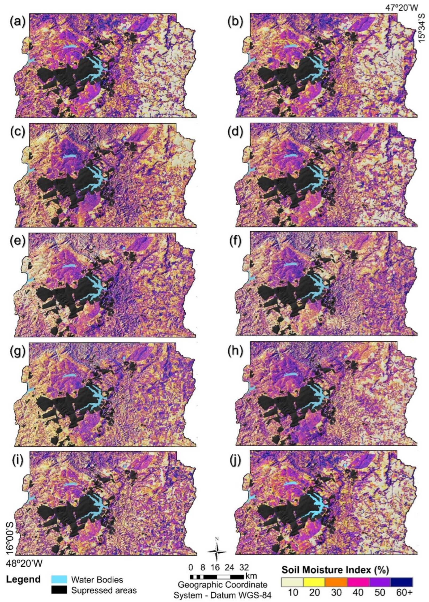
Figure 5.
Variation in soil moisture (SM) in time series and validation stage: (a) observed SM (green boxes) and predicted (yellow boxes) and daily rainfall (gray columns); (b) validation SM points (reference SM observed); (c) SM predicted by Random Forest algorithm. Where, FRha, Haplic Ferralsol; PTha, Haplic Plinthosol; FRro, Rhodic Ferralsol; ARdy, Dystric Arenosol; RGdy, Dystric Regosol; SD +, high standard deviation, SD -, Low standard deviation.
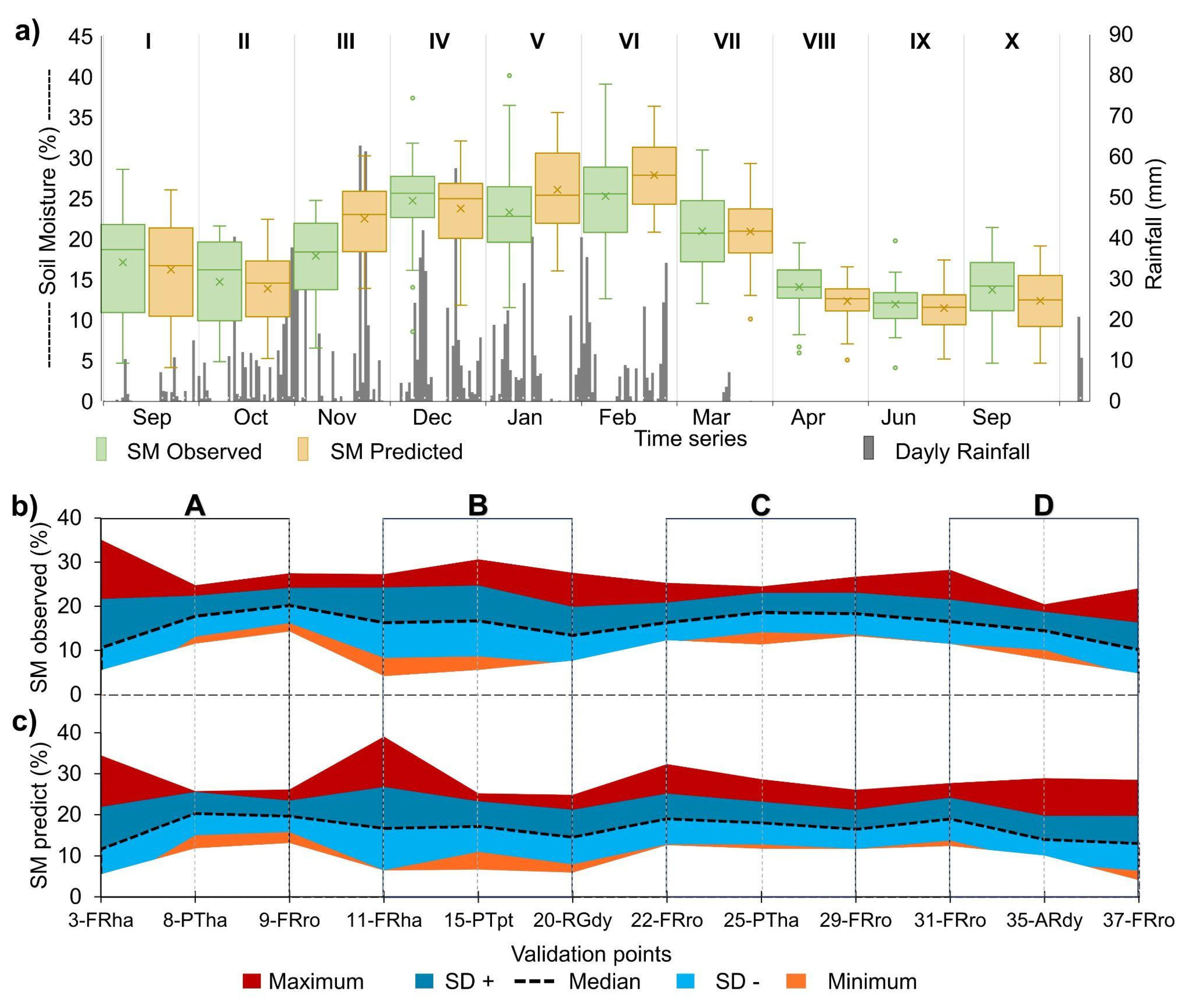
Figure 6.
Soil moisture variation in maps and time series chart. (a) soil moisture coefficient of variation (CV), (b) Relative Topsoil Moisture Index (RMSI), and (c) time series of predicted soil moisture variation coefficient and relative topsoil moisture curves.
Figure 6.
Soil moisture variation in maps and time series chart. (a) soil moisture coefficient of variation (CV), (b) Relative Topsoil Moisture Index (RMSI), and (c) time series of predicted soil moisture variation coefficient and relative topsoil moisture curves.
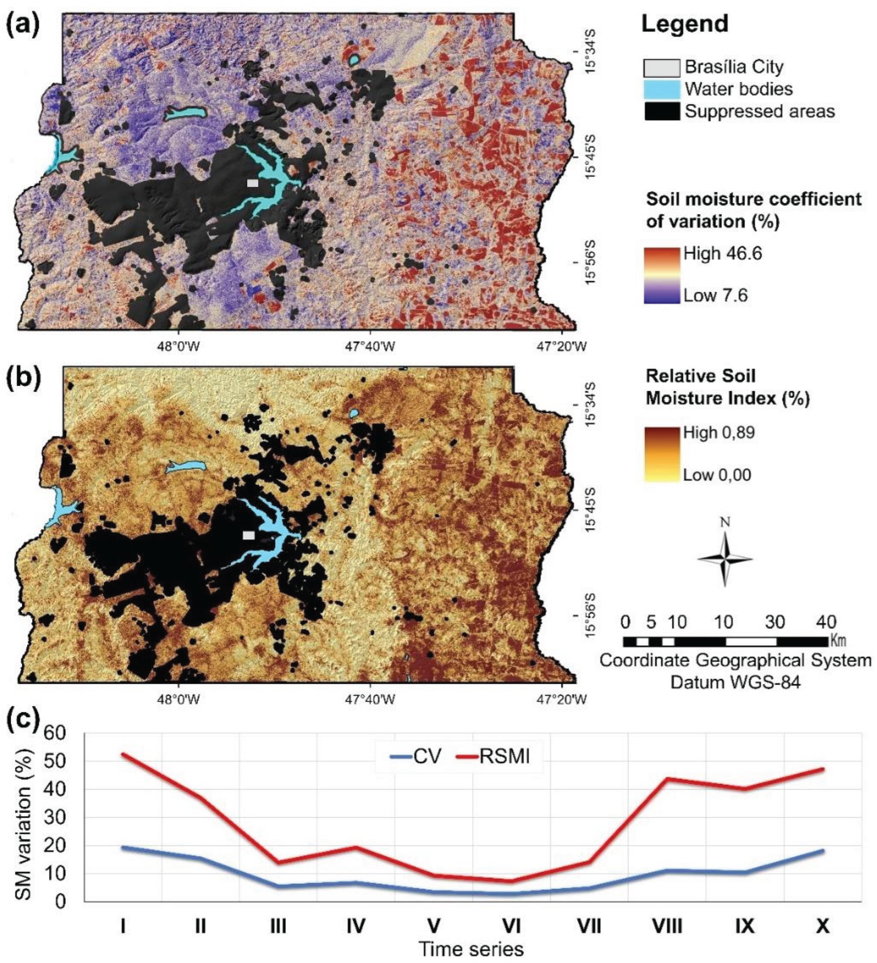

Table 1.
Date of Sentinel-1 time-series imagery and soil sampling.
| Series1 | I | II | III | IV | V | VI | VII | VIII | IX | X |
|---|---|---|---|---|---|---|---|---|---|---|
| Month | Oct | Oct | Nov | Dec | Jan | Feb | Mar | Apr | Jun | Sep |
| Day | 5th | 29th | 22th | 16th | 21th | 14th | 9th | 14th | 25th | 17th |
| Year | 2020 | 2020 | 2020 | 2020 | 2021 | 2021 | 2021 | 2021 | 2021 | 2021 |
1 The series refers to sampling dates, which served as a reference for Sentinel-1 acquisition and cloud-free Sentinel-2 for NDVI calculation.
Table 2.
Soil classes, texture, sample amount total, and distribution per established region.
| Soil Class 1 | Acronym | Texture ranging | Sample amount 2 | |||||
|---|---|---|---|---|---|---|---|---|
| A | B | C | D | T | ||||
| Dystric Rhodic Ferralsol | FR ro,dy | from very clayey to clayey | 4 | 3 | 4 | 5 | 16 | |
| Dystric Haplic Ferralsol | FR ha,dy | from very clayey to clayey | 1 | 2 | 2 | 5 | ||
| Petric Dystric Haplic Ferralsol | FR ha,pt | from very clayey to loam-clayey | 3 | 2 | 2 | 7 | ||
| Dystric Arenosol | AR dy | sandy | 1 | 1 | 1 | 3 | ||
| Dystric Regosol | RG dy | very clayey | 2 | 1 | 1 | 4 | ||
| Haplic Dystric Plinthosol | PT ha,dy | from very clayey to clayey | 3 | 2 | 3 | 8 | ||
| Petric Dystric Plinthosol | PT pt,dy | from very clayey to sand-loamy | 1 | 3 | 2 | 3 | 9 | |
1 Soil classes according to the IUSS Working Group WRB (2015); 2 Sample amounts per region (A, B, C, and D); and (T) the total of samples per soil class.
Table 4.
Metrics of modeling of SM via the Random Forest algorithm.
| N | F-1 | Training | Test | Validation | ||||||
|---|---|---|---|---|---|---|---|---|---|---|
| R2 | SE | RMSE | R2 | SE | RMSE | R2 | SE | RMSE | ||
| I | 0.54 | 0.95 | 0.02 | 0.04 | 0.95 | 0.01 | 0.01 | 0.81 | 0.02 | 0.03 |
| II | 0.81 | 0.84 | 0.02 | 0.04 | 0.88 | 0.02 | 0.04 | 0.78 | 0.03 | 0.09 |
| III | 0.58 | 0.86 | 0.02 | 0.04 | 0.84 | 0.02 | 0.04 | 0.74 | 0.03 | 0.09 |
| IV | 0.43 | 0.82 | 0.02 | 0.04 | 0.90 | 0.02 | 0.04 | 0.69 | 0.03 | 0.09 |
| V | 0.66 | 0.88 | 0.02 | 0.04 | 0.93 | 0.02 | 0.04 | 0.73 | 0.03 | 0.09 |
| VI | 0.57 | 0.87 | 0.03 | 0.09 | 0.82 | 0.03 | 0.09 | 0.60 | 0.04 | 0.16 |
| VII | 0.39 | 0.89 | 0.02 | 0.04 | 0.84 | 0.02 | 0.04 | 0.60 | 0.04 | 0.16 |
| VIII | 0.36 | 0.83 | 0.01 | 0.01 | 0.89 | 0.01 | 0.01 | 0.69 | 0.03 | 0.16 |
| IX | 0.24 | 0.86 | 0.01 | 0.01 | 0.88 | 0.01 | 0.01 | 0.70 | 0.02 | 0.04 |
| X | 0.33 | 0.90 | 0.02 | 0.04 | 0.92 | 0.01 | 0.01 | 0.72 | 0.02 | 0.04 |
| 0.49 | 0.87 | 0.02 | 0.02 | 0.89 | 0.02 | 0.02 | 0.71 | 0.03 | 0.10 | |
N—Serie number; R2—Coefficient of determination; SE—Standard error; RMSE—Root mean square error; —metrics mean.
Table 5.
Percentages of overlap between the variation in SM over the analyzed time series and soil classes, geomorphology, geology, and LULC maps.
Table 5.
Percentages of overlap between the variation in SM over the analyzed time series and soil classes, geomorphology, geology, and LULC maps.
| Legacy maps | Soil moisture variation classes (%) | |||||||
|---|---|---|---|---|---|---|---|---|
| Soil Class1 | 10 | 20 | 30 | 40 | 50 | 60 | 70+ | Subtotal |
| Rhodic Acrisol | 0.0 | 0.7 | 0.1 | 0.0 | 0.0 | 0.0 | 0.0 | 0.8 |
| Haplic Acrisol | 0.0 | 1.7 | 0.5 | 0.1 | 0.0 | 0.0 | 0.0 | 2.2 |
| Cambisol | 1.2 | 15.4 | 14.8 | 0.6 | 0.5 | 0.2 | 0.0 | 32.8 |
| Chernozems | 0.0 | 0.0 | 0.1 | 0.0 | 0.0 | 0.0 | 0.0 | 0.1 |
| Plinthosol | 0.0 | 0.1 | 0.0 | 0.0 | 0.0 | 0.0 | 0.0 | 0.1 |
| Rhodic Ferralsol | 4.4 | 15.7 | 14.4 | 4.9 | 1.6 | 0.2 | 0.1 | 41.2 |
| Haplic Ferralsol | 0.9 | 8.6 | 5.3 | 1.3 | 0.2 | 0.2 | 0.0 | 16.5 |
| Fluvisols | 0.0 | 0.2 | 0.0 | 0.0 | 0.0 | 0.0 | 0.0 | 0.2 |
| Arenosol | 0.0 | 0.4 | 0.1 | 0.0 | 0.0 | 0.0 | 0.0 | 0.5 |
| Nitisol | 0.0 | 0.7 | 0.7 | 0.0 | 0.0 | 0.0 | 0.0 | 1.4 |
| Haplic Plinthosol | 0.0 | 0.1 | 0.3 | 0.0 | 0.0 | 0.0 | 0.0 | 0.4 |
| Hydromorphic Soils | 0.0 | 2.3 | 1.2 | 0.1 | 0.0 | 0.0 | 0.0 | 3.7 |
| Geomorphological Surface (GS) 2 | 10 | 20 | 30 | 40 | 50 | 60 | 70+ | Subtotal |
| GS-I | 2.3 | 16.1 | 13.2 | 2.5 | 0.8 | 0.2 | 0.1 | 35.2 |
| GS-II | 2.1 | 15.0 | 12.2 | 2.3 | 0.7 | 0.2 | 0.1 | 32.7 |
| GS-III | 2.1 | 14.7 | 12.1 | 2.3 | 0.7 | 0.2 | 0.1 | 32.1 |
| Geological group 3 | 10 | 20 | 30 | 40 | 50 | 60 | 70+ | Subtotal |
| Araxá | 0.4 | 2.8 | 2.3 | 0.4 | 0.1 | 0.0 | 0.0 | 6.2 |
| Bambuí | 1.2 | 8.2 | 6.7 | 1.3 | 0.4 | 0.1 | 0.0 | 17.9 |
| Canastra | 1.1 | 7.8 | 6.4 | 1.2 | 0.4 | 0.1 | 0.0 | 17.0 |
| Paranoá | 3.9 | 27.0 | 22.1 | 4.2 | 1.3 | 0.4 | 0.1 | 58.9 |
| Land Use and Land Cover 4 | 10 | 20 | 30 | 40 | 50 | 60 | 70+ | Subtotal |
| Shrub field | 0.1 | 0.8 | 0.7 | 0.1 | 0.0 | 0.0 | 0.0 | 1.9 |
| Forest formation | 0.8 | 5.4 | 4.4 | 0.8 | 0.3 | 0.1 | 0.0 | 11.7 |
| Savannah | 0.2 | 1.3 | 1.0 | 0.2 | 0.1 | 0.0 | 0.0 | 2.8 |
| Mining | 0.1 | 0.9 | 0.7 | 0.1 | 0.0 | 0.0 | 0.0 | 1.9 |
| Perennial Crop | 1.2 | 8.5 | 7.0 | 1.3 | 0.4 | 0.1 | 0.0 | 18.6 |
| Temporary Crop | 0.1 | 0.9 | 0.7 | 0.1 | 0.0 | 0.0 | 0.0 | 2.0 |
| Pasture | 1.2 | 8.6 | 7.1 | 1.3 | 0.4 | 0.1 | 0.0 | 18.8 |
| Farming | 1.5 | 10.3 | 8.5 | 1.6 | 0.5 | 0.2 | 0.0 | 22.6 |
| Forestry | 1.3 | 9.1 | 7.4 | 1.4 | 0.5 | 0.1 | 0.0 | 19.8 |
| Subtotal | 6.5 | 45.8 | 37.5 | 7.1 | 2.3 | 0.7 | 0.1 | 100.0 |
1 Soil map (Reatto et al., 2004) adapted for IUSS Working Group WRB (2015); 2 Geomorphological map (Novaes-Pinto, 1987); 3 Geology map (Freitas-Silva & Campos, 1998) and 4 Land Use and Land Cover map (SEMA, 2021).
Disclaimer/Publisher’s Note: The statements, opinions and data contained in all publications are solely those of the individual author(s) and contributor(s) and not of MDPI and/or the editor(s). MDPI and/or the editor(s) disclaim responsibility for any injury to people or property resulting from any ideas, methods, instructions or products referred to in the content. |
© 2025 by the authors. Licensee MDPI, Basel, Switzerland. This article is an open access article distributed under the terms and conditions of the Creative Commons Attribution (CC BY) license (http://creativecommons.org/licenses/by/4.0/).
Copyright: This open access article is published under a Creative Commons CC BY 4.0 license, which permit the free download, distribution, and reuse, provided that the author and preprint are cited in any reuse.


