Submitted:
02 July 2025
Posted:
03 July 2025
You are already at the latest version
Abstract
Recently, time-series forecasting foundation models trained on large, diverse datasets have demonstrated robust zero-shot and few-shot capabilities. Given the ubiquity of time-series data in IoT, finance, and industrial applications, rigorous benchmarking is essential to assess their forecasting performance and overall value. In this study, our objective is to benchmark foundational models from Amazon, Salesforce, and Google against traditional statistical and deep learning baselines on both public and proprietary industrial datasets. We evaluate zero-shot, few-shot, and full-shot scenarios using metrics such as sMAPE and NMAE on fine-tuned models, ensuring reliable comparisons. All experiments are conducted with onTime, our dedicated open-source library that guarantees reproducibility, data privacy, and flexible configuration. Our results show that foundation models often outperform traditional methods with minimal dataset-specific tuning, underscoring their potential to simplify forecasting tasks and bridge performance gaps in data-scarce settings. Additionally, we address non-performance criteria—such as integration ease, model size, and inference/training time, which are critical for real-world deployment.
Keywords:
zero-shot forecasting
; foundation models
; model benchmarking
; time series analysis
; industrial applications
1. Introduction
The ability to forecast is one of the most prevalent uses of modeling. From weather forecasting to anomaly detection for specific industrial machines, accurately predicting the next few data points can significantly impact outcomes. Therefore, to be able to choose the right predictor is of capital importance.
In this paper, we explore some of the most recent modeling methods to predict time series. Those models are called foundation models and are becoming gradually more prevalent in the literature. For instance, notable examples include Chronos by Amazon, Moirai by Salesforce, and TimesFM by Google [1,2,3]. These models are based on methods similar to those used in foundation models for other applications, such as NLP.
Today, data scientists can rely on existing benchmarks such as GIFT-Eval or ProbTS to guide the selection of foundation models [4,5]. However, when applying these models to their own datasets, the results may differ from those reported. Furthermore, the benchmarks often consider the zero-shot scenario of those models, whereas the latter models can be trained and used in few-shot, or full-shot scenarios as well, leaving practitioners with an incomplete view of the models’ true potential.
Therefore, our research question revolves around the use of time series with foundation models, and is the following: "What is the performance of foundation models for time series forecasting and analysis on industrial datasets, particularly in the context of few-shot and zero-shot learning for specific use cases?"
Given the modernity of these models, this task involves challenges. Each model is rather large, requires significant computational power, has no unified interface, can treat time series differently (e.g. uni- or multi-variate, etc.), and metrics are difficult to choose.
In summary, the ability to position the performance of a given model on a specific dataset is of utmost importance. It enables practitioners to leverage these models and accelerates the technological transfer from academia to the industry.
The outline of our paper is structured within the framework of the scientific method. First, we explain the method based on a benchmarking tool that we developed. Second, we present the results of our benchmark. Finally, we discuss the implications of these results.
2. Materials and Methods
Our work’s objective is to evaluate the performance of recent foundation models in comparison with traditional methods. The following sections introduce our method, which aims to be as fair as possible. First, we present the choice of datasets, models, and metrics. Then, we introduce our method that fits different training and evaluation scenarios.
2.1. Datasets
Our datasets selection, presented in Table 1, aims to represent both reference data frequently used in academia and industrial data that no model has ever seen at training time. All academic datasets were sourced through the Darts Python library [6]. For consistency, a context window of 512 time steps is used across all datasets. We evaluate forecasting performance at horizons of 24, 48, 96, and 192 time steps, with a particular focus on the 96-step horizon in most experiments.
The Energy dataset covers hourly energy generation and weather in Spain from 2015 to 2018; eight constant features were removed. ETTh1 and ETTm1 contain hourly and 15-minute multivariate data from an electricity transformer, used to forecast oil temperature based on power load features. ExchangeRate contains daily exchange rates for eight countries from 1990 to 2016. Weather includes 21 weather indicators, such as temperature and humidity, recorded every 10 minutes in Germany during 2020. ZurichElectricity reports 15-minute resolution electricity consumption in Zurich up to 2022, combining household and business usage with interpolated weather data. HEIA reports hourly electricity consumption from eight buildings at our engineering school in Fribourg, Switzerland. Finally, MeteoSwiss provides 10-minute meteorological data from Fribourg/Grangeneuve, with features like pressure, wind, and humidity.
The datasets are split in a standard way, with 80% used for training and 20% for testing. For the deep learning models presented in the next section, the data are standardized to zero mean and unit variance using z-score normalization. In contrast, no normalization is applied to the statistical models, while for the foundation models, data normalization is handled internally by their respective implementations.
2.2. Models
Table 2 presents all models we considered for our benchmark. The 16 models can be split into three categories: (1) statistical, (2) deep learning, and (3) foundational. Those models have different characteristics: some are able to model multivariate data, while others focus on univariate series; their number of parameters varies; and one statistical model is included as a naive baseline for reference.
The hyperparameters of the deep learning models are optimized using the Optuna library in Python [20]. While each model has its own specific set of tunable parameters, several common hyperparameters—such as output chunk length, learning rate and its scheduler, dropout rate, and batch size—were consistently optimized across all models.
2.3. Metrics
The different metrics chosen for this benchmark must enable comparison across datasets and model characteristics (for instance, uni- vs multivariate output). Therefore, scale-independent metrics such as sMAPE and NMAE were chosen over traditional metrics like MSE or MAE.
sMAPE (Symmetric Mean Absolute Percentage Error) evaluates the relative error as a percentage, symmetrically penalizing over- and under-predictions. sMAPE is calculated as shown in Equation 1. Unlike traditional MAPE, sMAPE avoids division by zero and ensures that the metric remains bounded, making it well-suited for datasets with values near zero.
NMAE (Normalized Mean Absolute Error) expresses the total absolute error relative to the total magnitude of the true values. It provides an interpretable, scale-independent measure of forecast accuracy, particularly useful for comparing performance across datasets with different units or scales. NMAE is computed as shown in Equation 2.
By normalizing the absolute error by the total observed magnitude, NMAE avoids scale-related issues and allows a fair evaluation across different datasets or targets.
For multivariate forecasting, metrics are computed per component and averaged to yield a single aggregated performance score across all target variables.
2.4. Scenarios
Once the trio of models, datasets, and metrics is defined, different training scenarios are tested along two dimensions : (1) the amount of training data and (2) the prediction length.
The amount of training data can vary from none (zero-shot), a little (few-shots), to most of the dataset (full-shot). Statistical and deep-learning models have been trained in full-shot setting on the datasets from Section 2.1. Foundation models are first evaluated in a zero-shot setting, then fine-tuned for few-shot scenarios of varying training data proportion, and finally for full-shot. This dimension allows us to understand how effectively a model can capture patterns or characteristics within the data.
Regarding the prediction length, the lengths mentioned in Section 2.1 are considered (24, 48, 96, and 192 time-steps). This allows evaluating the ability of a model to capture dependencies as a function of time.
2.5. Evaluation Framework and Infrastructure
To create this benchmark, we developed an evaluation framework based on the onTime library [21]. This tool eases the development of all scenarios while increasing the certainty that experiments are executed in the exact same way. To define such experiments, the trio datasets, models, and metrics can be defined easily in a Python file. This framework is extensible via abstract classes, which allows a practitioner to specify a custom implementation.
While training is handled by each model’s implementation, evaluation is performed in a unified way across all models to ensure fair comparison. Specifically, a sliding window with a stride equal to the prediction horizon is used to generate multiple input–target samples from the test set. These are provided to the model after training, or directly in the case of zero-shot foundation models. Figure 1 illustrates this sampling process.
In terms of infrastructure, all experiments are performed on a Slurm cluster in version 24.05.3 with the following NVIDIA GPUs: (1) RTX A6000 with 48GB, (2) A40 with 48GB and (3) TITAN RTX with 24GB. Once all models are trained, a single GPU (A40) is used to compute all inference times, thus allowing a fair comparison.
3. Results
In this section, we present the results of the benchmark described in Section 2. First, we report the performance of the baseline models and compare them to the foundation models in a zero-shot setting (Section 3.1). Next, we analyze the performance of the foundation models across varying prediction horizons (Section 3.2). Finally, we evaluate the foundation models in few-shot settings, considering different proportions of the training data (Section 3.3).
3.1. Predictions Across Models
The baseline results from Table 3 feature deep learning and statistical models. The results are consistent across metrics, and TiDE provides the best predictions in most cases, followed by Naïve Seasonal and AutoARIMA.
In Table 4, we observe that foundation models perform better than the best baseline from Table 3. The best foundation models are Chronos Bolt Base, and Chronos Large, followed by Chronos Tiny and TimesFM. For some datasets, the performance across metrics shows a slight instability.
Figure 2 illustrates the trade-off between inference efficiency and forecasting error on the HEIA dataset. The bar chart (on the right) shows large differences in inference time across models: deep learning models are generally faster than foundation models, although lightweight variants like Chronos Bolt Tiny and Moirai Small also exhibit low inference times. In contrast, larger models such as Chronos Large and Moirai MoE Base are slower, as well as AutoARIMA and Exponential Smoothing.
The scatter plot (on the left) highlights that foundation models offer the best accuracy while maintaining competitive latency. Chronos Bolt and Moirai models represent a favorable trade-off, achieving both low error and fast inference.
3.2. Predictions Horizons
In terms of prediction horizon, Table 5 showcases the ability of models to predict different horizons. The best models align with the results from the previous Table 4. The awaited result is that the longer the prediction horizon, the more difficult it is to predict. However, when looking at the scores, the aforementioned statement is not always confirmed, which can be interpreted as instabilities difficult to characterize.
3.3. Few-Shot Learning with Various Data Proportions
Finally, we test the gain in score as a function of the proportion of the data seen by the model. Table 6 reports forecasting performance for 0% (zero-shot), 33%, 67%, and 100% (full-shot) scenarios. The results indicate that fine-tuning provides added value in most cases. However, Chronos Large appears to benefit less from fine-tuning compared to other models. Additionally, fine-tuning does not yield improvements when the data presents a more random character, which could indicate a data issue.
4. Discussion
In the context of this benchmark, we asked ourselves: What is the performance of foundation models for time series forecasting and analysis on industrial datasets, particularly in the context of few-shot and zero-shot learning for specific use cases?. To answer this question, we performed an extensive analysis of the models listed in Table 2 with an evaluation procedure testing cases such as datasets, prediction length, and data quantity.
The results presented in the previous section show the superiority of foundational models when compared with traditional methods in various contexts. First, as seen on Table 4, the latter models mostly provide better resulting metrics on prediction tasks. Second, as seen on Figure 2, when their size remains small, their inference speed is on par with the fastest traditional models. Third, when used in zero-shot settings, they do not require model-specific retraining.
However, such models are not a solution to all predictive needs. Having sizes varying from 8M to 700M parameters, their larger versions are computationally intensive and slow, limiting applications in resource-constrained contexts. Albeit, the smallest versions do provide great predictive performances compared to most baseline models (see Figure 2) within a very portable model, thus allowing for numerous applied usages.
When benchmarking, we noted interesting features of foundation models regarding (1) their prediction stability, (2) their prediction length performance, and (3) their fine-tuning process.
Regarding the prediction stability, when looking at the metrics across datasets, it seems like foundation models are more frequently specialized for some datasets (see Chronos Bolt Base) whereas baseline models (see TiDE and NaiveSeasonal) obtained great performance for 50% of the datasets. This seems slightly counterintuitive since one of the basic concepts of foundation models is to perform well across different datasets.
Concerning prediction performance, irregular behaviors have been observed across different prediction lengths. Indeed, longer predictions are usually harder to predict, and when looking at Table 5, some errors did decrease. The case of the Weather dataset is particularly special and may be due to the sampling length giving samples that are difficult to predict.
With respect to fine-tuning, such a process requires quite extensive knowledge, compute, and can deliver a wide range of results depending on the chosen dataset; e.g. marginal gains on the HEIA dataset and significant ones on the MeteoSwiss and ZurichElectricity datasets. Therefore, such a process should be done carefully and is, for now, limited to practitioners having access to great compute resources.
Finally, we can’t say that one foundation model is better than all others, but given our quantitative evaluation, Chronos seems to perform generally better. However, the testing of such models should also be done with a qualitative mindset and visual analysis, for instance, to validate their performance together with applied experts.
5. Conclusions
This study benchmarks foundation models for industrial time series forecasting, highlighting their superior zero-shot accuracy compared to traditional methods. Compact models, such as Chronos Bolt Tiny, provide an optimal balance of speed and performance, suitable for resource-constrained scenarios. However, larger models require substantial computational resources, and their performance varies across datasets and prediction horizons. Future work should focus on improving model stability, simplifying fine-tuning processes, and incorporating qualitative assessments to enhance practical usability.
Author Contributions
Conceptualization, B.P., F.M. and B.W.; methodology, B.P. and F.M.; software, B.P. and F.M.; validation, F.M. and B.W.; formal analysis, B.P.; investigation, B.P. and F.M.; resources, B.P., F.M. and B.W.; data curation, B.P.; writing—original draft preparation, F.M. and B.P.; writing—review and editing, F.M., B.P., B.W.; visualization, B.P.; supervision, B.W., F.M.; project administration, B.W.; funding acquisition, B.W. All authors have read and agreed to the published version of the manuscript.
Funding
This research is funded through a research grant of the University of Applied Sciences and Arts of Western Switzerland, HES-SO.
Data Availability Statement
Section 2.1 presents all datasets available in this study. The datasets Energy, ETTh1, ETTm1, ExchangeRate, Weather, and ZurichElectricity are available in Darts Python library [6]. The dataset MeteoSwiss is available on request from the authors.
Conflicts of Interest
The authors declare no conflicts of interest.
References
- Ansari, A.F.; Stella, L.; Turkmen, C.; Zhang, X.; Mercado, P.; Shen, H.; Shchur, O.; Rangapuram, S.S.; Pineda Arango, S.; Kapoor, S.; et al. Chronos: Learning the Language of Time Series. arXiv preprint arXiv:2403.07815 2024.
- Liu, X.; Liu, J.; Woo, G.; Aksu, T.; Liang, Y.; Zimmermann, R.; Liu, C.; Savarese, S.; Xiong, C.; Sahoo, D. Moirai-MoE: Empowering Time Series Foundation Models with Sparse Mixture of Experts, 2024, [arXiv:cs.LG/2410.10469].
- Das, A.; Kong, W.; Sen, R.; Zhou, Y. A decoder-only foundation model for time-series forecasting, 2024, [arXiv:cs.CL/2310.10688].
- Aksu, T.; Woo, G.; Liu, J.; Liu, X.; Liu, C.; Savarese, S.; Xiong, C.; Sahoo, D. GIFT-Eval: A Benchmark For General Time Series Forecasting Model Evaluation, 2024, [arXiv:cs.LG/2410.10393].
- Zhang, J.; Wen, X.; Zhang, Z.; Zheng, S.; Li, J.; Bian, J. ProbTS: Benchmarking Point and Distributional Forecasting across Diverse Prediction Horizons, 2024, [arXiv:cs.LG/2310.07446].
- Herzen, J.; Lässig, F.; Piazzetta, S.G.; Neuer, T.; Tafti, L.; Raille, G.; Pottelbergh, T.V.; Pasieka, M.; Skrodzki, A.; Huguenin, N.; et al. Darts: User-Friendly Modern Machine Learning for Time Series. Journal of Machine Learning Research 2022, 23, 1–6.
- Energy Consumption, Generation, Prices and Weather, 2019. Accessed: 2024-11-17.
- Zhou, H.; Zhang, S.; Peng, J.; Zhang, S.; Li, J.; Xiong, H.; Zhang, W. Informer: Beyond Efficient Transformer for Long Sequence Time-Series Forecasting. In Proceedings of the The Thirty-Fifth AAAI Conference on Artificial Intelligence, AAAI 2021, Virtual Conference. AAAI Press, 2021, Vol. 35, pp. 11106–11115.
- Lai, G.; Chang, W.C.; Yang, Y.; Liu, H. Modeling Long- and Short-Term Temporal Patterns with Deep Neural Networks. In Proceedings of the The 41st International ACM SIGIR Conference on Research & Development in Information Retrieval, New York, NY, USA, 2018; SIGIR ’18, p. 95–104. [CrossRef]
- Max Planck Institute for Biogeochemistry. Weather Data from the Max Planck Institute for Biogeochemistry, Jena, Germany. https://www.bgc-jena.mpg.de/wetter/, 2025. Accessed: 2025-05-16.
- Umwelt- und Gesundheitsschutz Zürich. Stündlich aktualisierte Meteodaten, seit 1992. https://data.stadt-zuerich.ch/dataset/ugz_meteodaten_stundenmittelwerte, 2025. Accessed: 2025-05-16.
- Elektrizitätswerk der Stadt Zürich. Viertelstundenwerte des Stromverbrauchs in den Netzebenen 5 und 7 in der Stadt Zürich, seit 2015. https://data.stadt-zuerich.ch/dataset/ewz_stromabgabe_netzebenen_stadt_zuerich, 2025. Accessed: 2025-05-16.
- MeteoSwiss. Federal Office of Meteorology and Climatology, 2024. Accessed: 2024-11-18.
- Hyndman, R.J.; Khandakar, Y. Automatic Time Series Forecasting: The forecast Package for R. Journal of Statistical Software 2008, 27, 1–22. [CrossRef]
- Cho, K.; van Merrienboer, B.; Gulcehre, C.; Bahdanau, D.; Bougares, F.; Schwenk, H.; Bengio, Y. Learning Phrase Representations using RNN Encoder-Decoder for Statistical Machine Translation, 2014, [arXiv:cs.CL/1406.1078].
- Das, A.; Kong, W.; Leach, A.; Mathur, S.; Sen, R.; Yu, R. Long-term Forecasting with TiDE: Time-series Dense Encoder, 2024, [arXiv:stat.ML/2304.08424].
- Lim, B.; Arık, S.Ö.; Loeff, N.; Pfister, T. Temporal Fusion Transformers for interpretable multi-horizon time series forecasting. International Journal of Forecasting 2021, 37, 1748–1764. [CrossRef]
- Chen, S.A.; Li, C.L.; Yoder, N.; Arik, S.O.; Pfister, T. TSMixer: An All-MLP Architecture for Time Series Forecasting, 2023, [arXiv:cs.LG/2303.06053].
- Woo, G.; Liu, C.; Kumar, A.; Xiong, C.; Savarese, S.; Sahoo, D. Unified Training of Universal Time Series Forecasting Transformers, 2024, [arXiv:cs.LG/2402.02592].
- Akiba, T.; Sano, S.; Yanase, T.; Ohta, T.; Koyama, M. Optuna: A Next-generation Hyperparameter Optimization Framework. In Proceedings of the Proceedings of the 25th ACM SIGKDD International Conference on Knowledge Discovery & Data Mining, New York, NY, USA, 2019; KDD ’19, p. 2623–2631. [CrossRef]
- ontime.re. onTime: Your Library to Work with Time Series. GitHub repository, 2024. https://github.com/ontime-re/ontime (accessed on 18.11.2024).
Figure 1.
Sliding window sampling on the test set. Each sample includes an input (context) and a target (ground truth for the prediction horizon).
Figure 1.
Sliding window sampling on the test set. Each sample includes an input (context) and a target (ground truth for the prediction horizon).
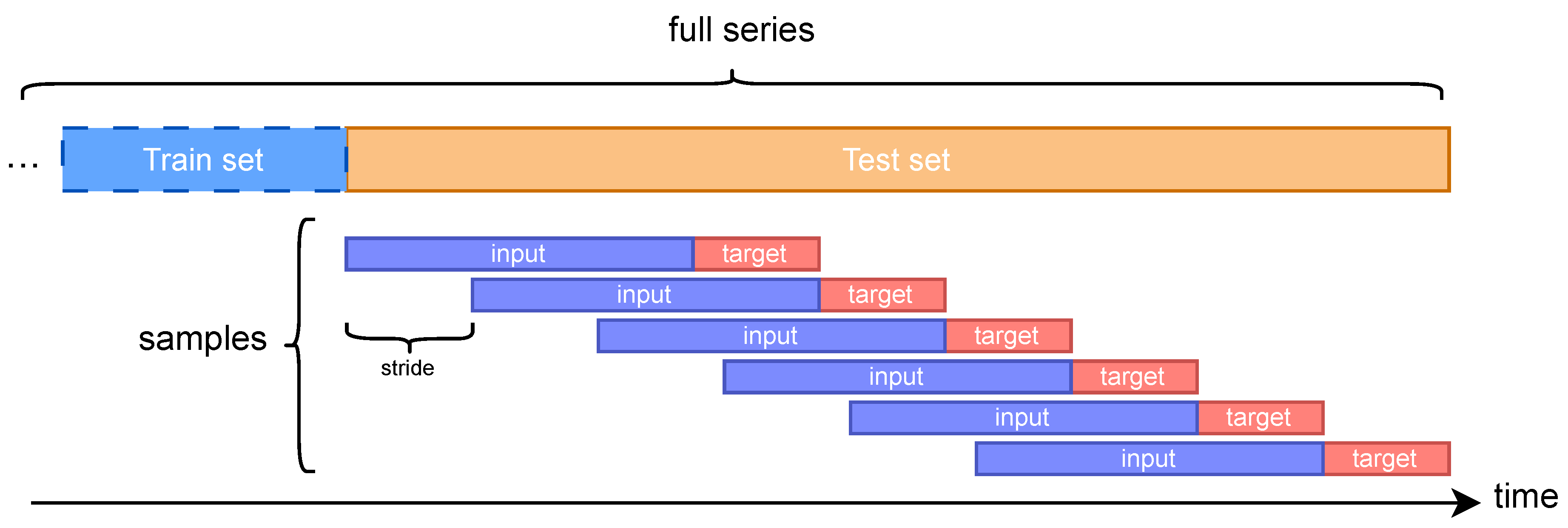
Figure 2.
Comparison of forecasting models trade-off between inference time (log scale) and forecasting accuracy measured by NMAE on the HEIA dataset.
Figure 2.
Comparison of forecasting models trade-off between inference time (log scale) and forecasting accuracy measured by NMAE on the HEIA dataset.
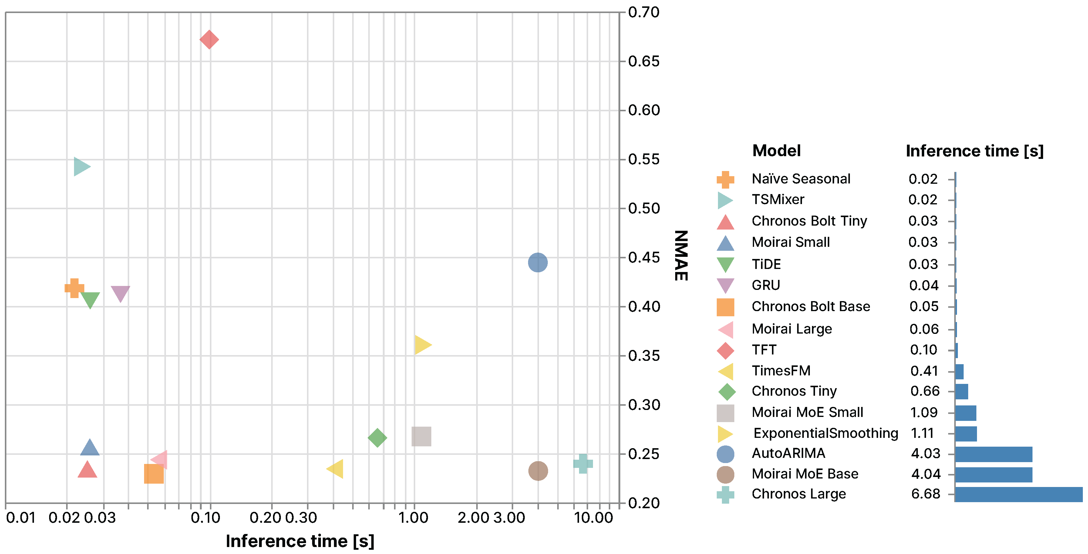

Table 1.
All datasets used to train the models. These datasets cover a wide range of use cases.
| Dataset | Type | # Features | Resolution | # Target Features | Size |
|---|---|---|---|---|---|
| Energy [7] | Academic | 20 | 1 hour | 1 (Total load) | 35,064 |
| ETTh1 [8] | Academic | 7 | 1 hour | 1 (Oil temp.) | 17,420 |
| ETTm1 [8] | Academic | 7 | 15 minutes | 1 (Oil temp.) | 69,680 |
| ExchangeRate [9] | Academic | 8 | 1 day | 8 (All) | 7,588 |
| Weather [10] | Academic | 21 | 10 minutes | 21 (All) | 52,704 |
| ZurichElectricity [11,12] | Academic | 10 | 15 minutes | 2 (Consumption) | 93,409 |
| HEIA1h | Industrial | 8 | 1 hour | 8 (All) | 11,664 |
| MeteoSwiss [13] | Industrial | 8 | 10 minutes | 24 (All) | 105,264 |
Table 2.
Overview of all models used for the benchmark. † These models are also finetuned.
| Model | Type | Prediction type | # Parameters |
|---|---|---|---|
| NaïveSeasonal | Statistical | Univariate | Not applicable |
| AutoARIMA [14] | Statistical | Univariate | < 100 |
| ExpotentialSmoothing | Statistical | Univariate | Not applicable |
| GRU [15] | Deep learning | Multivariate | 3-160K |
| TiDE [16] | Deep learning | Multivariate | 285K-8.5M |
| TFT [17] | Deep learning | Multivariate | 3-36K |
| TSMixer [18] | Deep learning | Multivariate | 19-931K |
| Chronos Tiny† [1] | Foundation | Univariate | 8M |
| Chronos Large† [1] | Foundation | Univariate | 710M |
| Chronos Bolt Small [1] | Foundation | Univariate | 48M |
| Chronos Bolt Base [1] | Foundation | Univariate | 205M |
| Moirai small† [19] | Foundation | Multivariate | 14M |
| Moirai large† [19] | Foundation | Multivariate | 311M |
| Moirai MoE Small [2] | Foundation | Multivariate | 117M |
| Moirai MoE Base [2] | Foundation | Multivariate | 935M |
| TimesFM [3] | Foundation | Univariate | 500M |
Table 3.
Forecasting performance of baseline models on a prediction horizon of 96 time steps. The best score per row is in bold, the second best is underlined. † ES = Exponential Smoothing.
Table 3.
Forecasting performance of baseline models on a prediction horizon of 96 time steps. The best score per row is in bold, the second best is underlined. † ES = Exponential Smoothing.
| Deep learning | Statistical | |||||||
|---|---|---|---|---|---|---|---|---|
| Metrics | GRU | TFT | TiDE | TSMixer | Naive Seasonal | AutoARIMA | ES† | |
| Energy | sMAPE | 13.49 | 15.25 | 8.102 | 9.724 | 20.56 | 13.34 | 22.67 |
| NMAE | .1332 | .1507 | .0825 | .0952 | .1946 | .1318 | .2215 | |
| ETTh1 | sMAPE | 35.00 | 47.15 | 40.11 | 38.13 | 34.49 | 33.60 | 35.80 |
| NMAE | .4003 | .6310 | .4097 | .5261 | .3627 | .3526 | .3781 | |
| ETTm1 | sMAPE | 32.11 | 41.53 | 55.02 | 26.05 | 22.27 | 23.59 | 24.55 |
| NMAE | .3190 | .6568 | 1.040 | .2950 | .2325 | .2369 | .2462 | |
| ExchangeRate | sMAPE | 15.55 | 18.06 | 11.45 | 15.34 | 2.336 | 2.514 | 2.537 |
| NMAE | .1428 | .1631 | .1049 | .1416 | .0234 | .0249 | .0252 | |
| Weather | sMAPE | 79.09 | 81.48 | 62.53 | 65.67 | 54.58 | 61.77 | 66.82 |
| NMAE | 250.0 | 223.5 | 50.21 | 39.41 | 1.073 | 10.85 | 38.16 | |
| ZurichElectricity | sMAPE | 14.20 | 21.87 | 5.395 | 8.260 | 18.53 | 18.49 | 23.39 |
| NMAE | .1401 | .2160 | .0548 | .0835 | .1871 | .1858 | .2416 | |
| HEIA | sMAPE | 42.26 | 52.47 | 29.56 | 39.48 | 39.99 | 41.65 | 31.28 |
| NMAE | .5380 | .6706 | .3240 | .5422 | .4182 | .4445 | .3606 | |
| MeteoSwiss | sMAPE | 75.64 | 89.08 | 64.64 | 80.11 | 68.98 | 71.96 | 72.76 |
| NMAE | 1.641 | 2.170 | 1.085 | 1.810 | 2.152 | 1.768 | 2.664 | |
Table 4.
Forecasting performance of foundation models on a prediction horizon of 96 time steps, evaluated in a zero-shot setting. Best baselines scores from Table 3 are also reported. The best score per row is in bold, the second best is underlined. † TFM = TimesFM, ‡ BB = Best baselines.
Table 4.
Forecasting performance of foundation models on a prediction horizon of 96 time steps, evaluated in a zero-shot setting. Best baselines scores from Table 3 are also reported. The best score per row is in bold, the second best is underlined. † TFM = TimesFM, ‡ BB = Best baselines.
| Moirai | Moirai-MoE | Chronos | Chronos Bolt | TFM† | BB‡ | ||||||
|---|---|---|---|---|---|---|---|---|---|---|---|
| Metrics | Small | Large | Small | Base | Tiny | Large | Tiny | Base | |||
| Energy | sMAPE | 7.360 | 7.134 | 7.088 | 7.062 | 7.508 | 4.854 | 6.183 | 5.095 | 7.035 | 8.102 |
| NMAE | .0744 | .0718 | .0719 | .0718 | .0751 | .0491 | .0622 | .0511 | .0708 | .0825 | |
| ETTh1 | sMAPE | 32.64 | 34.61 | 33.25 | 34.04 | 31.15 | 30.68 | 31.95 | 30.56 | 31.40 | 33.60 |
| NMAE | .3382 | .3344 | .3333 | .3370 | .3242 | .3217 | .3408 | .3334 | .3231 | .3526 | |
| ETTm1 | sMAPE | 23.66 | 24.64 | 24.78 | 23.64 | 22.95 | 21.61 | 21.58 | 22.40 | 22.45 | 22.27 |
| NMAE | .2461 | .2658 | .2569 | .2488 | .2347 | .2303 | .2346 | .2329 | .2521 | .2325 | |
| ExchangeRate | sMAPE | 2.505 | 2.687 | 2.470 | 2.535 | 2.714 | 2.583 | 2.412 | 2.552 | 2.565 | 2.336 |
| NMAE | .0251 | .0273 | .0248 | .0255 | .0270 | .0260 | .0242 | .0255 | .0256 | .0234 | |
| Weather | sMAPE | 64.20 | 64.43 | 62.01 | 59.47 | 63.47 | 61.83 | 62.40 | 61.81 | 45.05 | 54.58 |
| NMAE | 2.663 | 9.052 | 11.05 | 5.192 | 13.03 | .4987 | 6.455 | 4.629 | 1.243 | 1.073 | |
| ZurichElectricity | sMAPE | 17.92 | 18.06 | 17.30 | 15.63 | 8.368 | 6.119 | 5.635 | 4.177 | 7.292 | 5.395 |
| NMAE | .1769 | .1804 | .1727 | .1540 | .0872 | .0639 | .0592 | .0440 | .0768 | .0548 | |
| HEIA | sMAPE | 22.74 | 20.89 | 23.31 | 20.20 | 23.33 | 20.73 | 20.37 | 19.71 | 20.67 | 29.56 |
| NMAE | .2570 | .2423 | .2670 | .2321 | .2687 | .2411 | .2343 | .2294 | .2343 | .3240 | |
| MeteoSwiss | sMAPE | 67.72 | 66.98 | 66.14 | 66.49 | 67.99 | 62.95 | 67.58 | 65.18 | 62.74 | 64.64 |
| NMAE | .8146 | 1.488 | 2.442 | 1.173 | 1.657 | 1.662 | .9932 | 1.377 | .9777 | 1.085 | |
Table 5.
Forecasting performance of foundation models on different prediction horizons, evaluated in a zero-shot setting. NMAE is reported. The best score per row is in bold, the second best is underlined. †TFM = TimesFM.
Table 5.
Forecasting performance of foundation models on different prediction horizons, evaluated in a zero-shot setting. NMAE is reported. The best score per row is in bold, the second best is underlined. †TFM = TimesFM.
| Moirai | Moirai-MoE | Chronos | Chronos Bolt | TFM† | ||||||
|---|---|---|---|---|---|---|---|---|---|---|
| Horizons | Small | Large | Small | Base | Tiny | Large | Tiny | Base | ||
| Energy | 24 | .0643 | .0592 | .0591 | .0528 | .0563 | .0338 | .0503 | .0385 | .0589 |
| 48 | .0719 | .0678 | .0678 | .0628 | .0678 | .0414 | .0587 | .0442 | .0676 | |
| 96 | .0744 | .0718 | .0719 | .0718 | .0751 | .0491 | .0622 | .0511 | .0708 | |
| 192 | .0773 | .0755 | .0746 | .0802 | .0754 | .0529 | .0646 | .0556 | .0734 | |
| ETTh1 | 24 | .2048 | .2104 | .1970 | .2021 | .2011 | .2074 | .1999 | .1944 | .2077 |
| 48 | .2619 | .2713 | .2503 | .2547 | .2447 | .2490 | .2495 | .2517 | .2536 | |
| 96 | .3382 | .3344 | .3333 | .3370 | .3242 | .3217 | .3408 | .3334 | .3231 | |
| 192 | .2883 | .2969 | .3063 | .2905 | .2849 | .2838 | .3070 | .2870 | .2784 | |
| ETTm1 | 24 | .1616 | .1967 | .1752 | .1755 | .1796 | .1446 | .1479 | .1443 | .1643 |
| 48 | .2515 | .2742 | .2574 | .2571 | .2382 | .2166 | .2397 | .2307 | .2594 | |
| 96 | .2461 | .2658 | .2569 | .2488 | .2347 | .2303 | .2346 | .2329 | .2521 | |
| 192 | .2917 | .3094 | .3055 | .3007 | .2950 | .2870 | .3008 | .3017 | .2977 | |
| ExchangeRate | 24 | .0138 | .0133 | .0128 | .0130 | .0140 | .0136 | .0131 | .0136 | .0132 |
| 48 | .0177 | .0179 | .0171 | .0174 | .0186 | .0184 | .0170 | .0182 | .0180 | |
| 96 | .0251 | .0273 | .0248 | .0255 | .0270 | .0260 | .0242 | .0255 | .0256 | |
| 192 | .0350 | .0472 | .0394 | .0397 | .0406 | .0375 | .0340 | .0343 | .0346 | |
| Weather | 24 | .8605 | .4102 | .5990 | .8083 | 2.260 | .3976 | 2.760 | .6189 | .6271 |
| 48 | 2.915 | 1.317 | 6.538 | 7.237 | 1.779 | .9095 | 6.655 | 1.919 | 1.834 | |
| 96 | 2.663 | 9.052 | 11.05 | 5.192 | 13.03 | .4987 | 6.455 | 4.629 | 1.243 | |
| 192 | .5276 | .6359 | .8007 | .7821 | .7816 | .5519 | .6735 | .5559 | .6298 | |
| Horizons | Small | Large | Small | Base | Tiny | Large | Tiny | Base | ||
| ZurichElectricity | 24 | .0883 | .0758 | .0721 | .0596 | .0339 | .0244 | .0292 | .0233 | .0316 |
| 48 | .1576 | .1413 | .1403 | .1076 | .0501 | .0297 | .0348 | .0289 | .0441 | |
| 96 | .1769 | .1804 | .1727 | .1540 | .0872 | .0639 | .0592 | .0440 | .0768 | |
| 192 | .1757 | .1838 | .1752 | .1621 | .1056 | .0825 | .0667 | .0501 | .0926 | |
| HEIA | 24 | .2220 | .1959 | .2131 | .1924 | .2123 | .1837 | .1998 | .1937 | .2013 |
| 48 | .2459 | .2177 | .2479 | .2111 | .2322 | .2086 | .2173 | .2098 | .2206 | |
| 96 | .2570 | .2423 | .2670 | .2321 | .2687 | .2411 | .2343 | .2294 | .2343 | |
| 192 | .2687 | .2659 | .2807 | .2467 | .2762 | .2540 | .2437 | .2408 | .2507 | |
| MeteoSwiss | 24 | .6949 | .8155 | .8457 | .6222 | .7558 | .7167 | .6576 | .8176 | .6057 |
| 48 | 1.153 | 1.441 | 1.771 | 1.016 | 1.457 | 1.297 | 1.045 | 1.346 | .9871 | |
| 96 | .8146 | 1.488 | 2.442 | 1.173 | 1.657 | 1.662 | .9932 | 1.377 | .9777 | |
| 192 | 1.226 | 1.530 | 1.850 | 1.898 | 1.584 | 1.374 | 1.295 | 1.231 | 1.336 | |
Table 6.
Forecasting performance of finetuned foundation models using different proportions of available training data from 0% (zero-shot) to 100% (full-shot). NMAE is reported. The best score for a given dataset and model is shown in bold. The overall best score for each dataset across all models is highlighted in bold red, and the second-best in underlined red.
| Moirai | Chronos | ||||
|---|---|---|---|---|---|
| Proportions | Small | Large | Tiny | Large | |
| Energy | 0% | .0744 | .0718 | .0751 | .0491 |
| 33% | .0727 | .0704 | .0649 | .0549 | |
| 67% | .0667 | .0658 | .0594 | .0495 | |
| 100% | .0687 | .0661 | .0599 | .0445 | |
| ETTh1 | 0% | .3382 | .3344 | .3242 | .3217 |
| 33% | .3146 | .3307 | .3315 | .3161 | |
| 67% | .3173 | .3167 | .3157 | .3272 | |
| 100% | .3127 | .3346 | .3099 | .3460 | |
| ETTm1 | 0% | .2461 | .2658 | .2347 | .2303 |
| 33% | .2404 | .3616 | .2459 | .2540 | |
| 67% | .2686 | .3693 | .2484 | .2754 | |
| 100% | .2437 | .2558 | .2198 | .2308 | |
| ExchangeRate | 0% | .0251 | .0273 | .0270 | .0260 |
| 33% | .0282 | .0694 | .0319 | .0319 | |
| 67% | .0250 | .0360 | .0285 | .0299 | |
| 100% | .0285 | .0779 | .0251 | .0302 | |
| Weather | 0% | 2.663 | 9.052 | 13.03 | .4987 |
| 33% | 3.793 | 6.041 | 2.053 | .9532 | |
| 67% | 6.670 | 2.425 | 1.670 | 3.274 | |
| 100% | 2.459 | 3.703 | 8.644 | 5.433 | |
| ZurichElectricity | 0% | .1769 | .1804 | .0872 | .0639 |
| 33% | .0482 | .0475 | .0326 | .0295 | |
| 67% | .0419 | .0526 | .0323 | .0277 | |
| 100% | .0499 | .0535 | .0333 | .0265 | |
| HEIA | 0% | .2570 | .2423 | .2687 | .2411 |
| 33% | .2631 | .2736 | .3271 | .2574 | |
| 67% | .2991 | .2920 | .2981 | .2488 | |
| 100% | .2653 | .2728 | .2494 | .2420 | |
| MeteoSwiss | 0% | .8146 | 1.488 | 1.657 | 1.662 |
| 33% | .5650 | .6690 | .6111 | .9706 | |
| 67% | .4954 | .4532 | 1.446 | .7739 | |
| 100% | .5396 | .5316 | .7382 | .6285 | |
Disclaimer/Publisher’s Note: The statements, opinions and data contained in all publications are solely those of the individual author(s) and contributor(s) and not of MDPI and/or the editor(s). MDPI and/or the editor(s) disclaim responsibility for any injury to people or property resulting from any ideas, methods, instructions or products referred to in the content. |
© 2025 by the authors. Licensee MDPI, Basel, Switzerland. This article is an open access article distributed under the terms and conditions of the Creative Commons Attribution (CC BY) license (http://creativecommons.org/licenses/by/4.0/).
Copyright: This open access article is published under a Creative Commons CC BY 4.0 license, which permit the free download, distribution, and reuse, provided that the author and preprint are cited in any reuse.


