Submitted:
23 January 2026
Posted:
27 January 2026
Read the latest preprint version here
Abstract
We present an updated formulation of the Spectral Bounded Vacuum (SBV) model, in which the quantum vacuum is described as a dynamically bounded spec- trum with physically motivated infrared and ultraviolet limits, linked to the ther- mal and hadronic evolution of the Universe. In this framework, the present-epoch vacuum energy arises within a spectrally bounded description from a balance be- tween spectral contribution and time-dependent damping, reflecting the influence of gravitation, thermodynamic (entropic) processes, and hadronic interactions. The characteristic spectral scale is determined by the geometric mean of the infrared and ultraviolet boundaries, leading to a robust scaling law without fine-tuning. A nu- merical evaluation with standard parameters for the current epoch yields a vacuum energy density consistent with the observed cosmological constant. The model is extended with the Quantum Entropic Vacuum (QEV), in which the entropic con- tribution of the vacuum is explicitly included as a dynamic component. The QEV picture describes how fluctuations in quantum entropy contribute to the tem- poral evolution of the vacuum energy, offering an additional explanation for the stability of the cosmological constant at late times. Thermal physics enters the model only indirectly, by setting an effective infrared scale that limits the range of vacuum modes which remain physically relevant in a thermally structured universe.
Keywords:
vacuum energy
; cosmological constant problem
; spectral bounded vacuum (SBV)
; quantum entropic vacuum (QEV)
; spectral cutoff
; quantum field theory in curved space vacuum energy
; quantum entropic vacuum
; cosmology
; casimir effect
; effective field theory
1. Introduction
The observed acceleration of the Universe is commonly modeled by a cosmological constant , yet its apparent smallness compared to naive quantum-field expectations remains puzzling. Rather than seeking an origin narrative for vacuum energy or an extended early-time dynamics, this work focuses strictly on a present-day description of the vacuum state: a phenomenological, physics-grounded framework that identifies natural spectral bounds and their consequences for the current energy density relevant to gravity.
Two guiding principles motivate our approach. First, laboratory and astrophysical physics already provide robust characteristic scales. In particular, the confinement scale of quantum chromodynamics (QCD) suggests a natural ultraviolet (UV) boundary for modes that can coherently contribute to the gravitationally active vacuum sector, while thermodynamic or entropic considerations suggest an infrared (IR) boundary for the longest relevant wavelengths. Second, once such bounds are admitted on physical grounds, dimensional analysis and a mild regularity requirement lead to a simple and robust scaling of the present-day vacuum energy density with a single geometric length scale.
This paper develops that late-time, present-epoch picture in a way that is intentionally diagnostic rather than definitive. At the background level, the framework reproduces low-redshift kinematics (e.g., and ) close to flat-CDM for reasonable choices of the bounding scales, without invoking fine-tuned parameters or assumptions about high-redshift evolution. On galactic scales, the same present-time perspective can be mapped into rotation-curve phenomenology through a small set of interpretable contributions. Importantly, the proposal is directly testable in the laboratory: we formulate photonic and radiometric observables via an impedance-invariant spectral window and a band-integrated measure , enabling null tests using optical, radiometric, or Casimir-type platforms.
We emphasize that the scope of this paper is deliberately limited: we do not attempt a full cosmological likelihood analysis nor a theory of origin for vacuum energy. Instead, we articulate a coherent present-time framework, grounded in known physics and observations, which yields clear diagnostics and falsifiability criteria that can be constrained by existing data and near-term experiments. The mathematical formulation begins in Sec. Section 3, after clarifying the physical scope in Sec. Section 2.
2. Present Framework and Physical Scope
This work is confined to the present-day vacuum state (late-time, ). Our objective is not to reconstruct a dynamical history or propose an origin theory, but to provide a physically realistic description of the current spectral and energetic properties of the vacuum sector that are relevant for gravity.
We assume that the effective vacuum spectrum is bounded by natural, well-motivated scales: an ultraviolet (UV) limit associated with QCD confinement (fixing a characteristic short length) and an infrared (IR) boundary associated with thermal or entropic considerations (fixing a characteristic long length). Within these bounds, the vacuum energy density takes a robust dimensional form
where L is the geometric mean of the UV and IR cutoffs and . All quantitative statements in this paper refer to this present-epoch configuration.
The framework is intended as a diagnostic description rather than a replacement for CDM or an account of early-universe physics. In the late-time regime, a spectrally bounded vacuum can (i) reproduce key background kinematics at low z to within a few percent of flat-CDM for plausible bounding scales, (ii) inform galaxy-scale phenomenology using a small number of interpretable contributions, and (iii) admit direct laboratory tests through photonic and radiometric observables. To make the latter operational, we employ an impedance-invariant spectral window and its band-integrated measure , which together provide platform-agnostic null tests (e.g., optical cavities/interferometers, radiometric measurements, or Casimir-type setups).
Accordingly, this paper should be read as a physically grounded present-time proposal—not a proof of origin—that defines a coherent, testable picture of vacuum energy at . The spectral construction and its mathematical consequences are developed in Sec. Section 3, while late-time diagnostics and laboratory connections are summarized where appropriate.
3. Spectral Formulation
3.1. Damping Budget and Uncertainties
We split the integrated damping as follows:
where Eq. (1) follows from adiabatic FRW expansion, captures entropic/thermal suppression across particle thresholds, and the Gaussian in Eq. () models a localized hadronic damping centered near .A representative calibration is , , (total ).
Small variations propagate as .

Table 1.
Illustrative damping budget and modest variations. Changes of e–folds shift by factors , remaining within the tolerance absorbed by and the kernel factor .
Table 1.
Illustrative damping budget and modest variations. Changes of e–folds shift by factors , remaining within the tolerance absorbed by and the kernel factor .
| Scenario | |||
|---|---|---|---|
| Baseline | 25 | 46 | 30 |
| IR–softer (more thermal) | 25 | 48 | 28 |
| Narrower hadronic peak | 25 | 45 | 28 |
| Wider hadronic peak | 25 | 45 | 32 |
| Total (baseline / variants) | 101 / 101–103 | ||
3.2. Late-Time Calibration
With fm and one has and, using Eq. (A5), the spectral scaling . Matching the observed late-time density fixes the dimensionless normalization via
;
for the fiducial this yields (the large value reflects the integrated damping factor ), while the smallness of relative to hadronic scales is explained by the integrated damping factor in Eq. (13). This SBV+QEV picture thus ties the present value of the cosmological constant to natural spectral bounds and to the entropic, hadronic, and gravitational history of the universe.
3.3. Summary of Revisions (v2)
This updated version of the paper formalizes the Spectral Bounded Vacuum (SBV) framework and introduces the Quantum Entropic Vacuum (QEV) extension to describe time-dependent damping of the vacuum energy. Analytical derivations of the bounded integral, numerical evaluations consistent with the cosmological constant, and several new figures and tables have been added. The normalization and dimensional analysis have been clarified, and an Observational Outlook section connects the theory to cosmological and laboratory-scale tests. References have been expanded, including a citation to the previous version (v1) of this work.
3.4. Summary of Scope and Results
The formulation developed above provides a concise, physically grounded description of the present-day vacuum state. Within the bounded spectral framework, the vacuum energy density scales as with linking quantum and thermodynamic length scales through a single geometric mean. When the ultraviolet cutoff is associated with the QCD confinement scale and the infrared limit with a thermal boundary near the current background temperature, the resulting naturally falls in the observed cosmological range.
At the background level, the model reproduces late-time expansion diagnostics, the dimensionless Hubble function , the deceleration parameter , and the transition redshift , that remain within a few percent of flat-CDM for physically plausible values of . No joint cosmological likelihood or early-universe assumptions are invoked; the emphasis is purely diagnostic for the present epoch ().
On smaller scales, the same parameter configuration can be mapped to galaxy rotation-curve phenomenology through a minimal set of interpretable contributions: a Newtonian term, a thermal-lift component, an entropic plateau, and a weak hadronic floor related to residual QCD effects. The combination reproduces typical high-quality rotation curves (e.g., NGC 3198) without per-object fine-tuning.
Finally, the framework yields direct laboratory observables. Using an impedance-invariant spectral window and its band-integrated measure , one can test the bounded-vacuum hypothesis through optical, radiometric, or Casimir-type experiments. These provide falsifiability criteria, for example, limits on or on deviations of and at the percent level, that anchor the model to measurable present-time quantities.
In summary, the spectral bounded vacuum formalism offers a coherent and testable picture of the vacuum energy at the current epoch: dimensionally robust, observationally constrained, and open to further refinement through ongoing astrophysical and laboratory measurements.
The results summarized above define the present-epoch behavior of a spectrally bounded vacuum and establish its immediate observational consequences. The remaining task is to translate these internal relations into empirical diagnostics and potential signatures. The following section therefore outlines the key observational and experimental avenues, from low-z cosmological measurements to laboratory photonic tests, that can either support or falsify this present-time framework.
4. Bounding Principles and Evidence
In this section we collect proof-style justifications for the ultraviolet (UV) and infrared (IR) bounds that enter the QEV window and for the narrower hadronic band used for local (in-hadron) contributions.
4.1. UV Bound from Confinement (QCD)
Proposition 1 (Confinement bound).
In non-Abelian SU(3) gauge theory at low temperature (), the Wilson-loop area law implies a linear static potential with string tension [23,24]. Consequently, color flux is localized into tubes of transverse size , and vacuum modes with do not propagate as free degrees of freedom. Hence a natural UV cutoff for the spectral vacuum integral is
Corollary 1 (Hadronic local band).
4.2. IR Bound from Thermodynamics, Entropy, and Expansion
The infrared scale entering the spectral window is motivated by thermodynamic and entropic considerations, but it does not represent a fundamental property of the vacuum itself. Rather, it reflects the thermal structuring of the late-time universe and its influence on which long-wavelength modes remain physically relevant.
In an expanding universe with temperature , thermal noise and entropy production effectively suppress the observational and gravitational relevance of vacuum modes with wavelengths much larger than the thermal coherence scale. This motivates the introduction of an effective infrared wavelength
which parametrizes the longest wavelengths that can contribute coherently under given thermal conditions.
Importantly, this infrared scale should be interpreted as a smooth, context-dependent selection boundary rather than a sharp cutoff or phase transition. In the late-time regime, where , the evolution of slows, leading to an approximately constant spectral window and a stable contribution to the vacuum energy density.
4.3. Mathematical Convergence of the Spectral Integral
Proposition 3 (Convergence).
For
with bounded , and any integrand with , the spectral integral
converges absolutely for all t and is dominated near (Laplace method). In particular, the QEV choice with the double-exponential kernel is well-posed [16].
4.4. Kernel Exponents and Robustness
The symmetric choice yields the closed-form integral with , making analytic control straightforward. Alternative exponents provide smoother or sharper UV/IR suppression but change the prefactor only by order-unity factors. This is illustrated by our spectral plot: the peak remains anchored near and the -law is unaffected. In practice, moderate changes in can be absorbed by a compensating shift in without invoking fine-tuning.
5. Dynamic Spectral Framework
We begin from the bounded spectral representation [16]
with a double-exponential suppression kernel [16]
To incorporate the time evolution of the vacuum, we promote this to a dynamic kernel:
where and represent hadronic and gravitational damping, respectively. The time dependence follows standard thermodynamics [6] and cosmic cooling inferred from CMB measurements [21]. The thermal/entropic evolution is captured through the time dependence of the infrared bound .
5.1. Hadronic and Gravitational Damping
The hadronic term peaks near the QCD transition temperature (see[15,23,24]):
while the gravitational (Hubble) damping term follows ref. [4].
The total effective damping rate is then
Here and is a dimensionless coupling; is the cumulative gravitational damping contributing to .
6. Dynamical QEV Model
The time evolution of the vacuum energy density obeys a continuity relation
with the formal solution
In the cosmic expansion, , giving
When at late times, the vacuum density approaches a constant and the equation-of-state parameter , consistent with CMB and large-scale-structure constraints[21].
7. Results and Discussion
The QEV framework developed here should be understood in its baseline propagation-only formulation, as specified in Appendix F. In this minimal realization, thermal physics does not enter through explicit dissipation or decay of vacuum energy. In particular, the thermal damping channel is set to zero,
and no microphysical energy exchange between matter, radiation, and the vacuum is assumed.
Instead, temperature enters solely through the effective propagation scale of the infrared sector, encoded in the time dependence of the infrared wavelength
which parametrizes the longest vacuum modes that remain physically relevant in a thermally structured universe.
Interpretation (propagation-only, no vacuum transition).
Within this baseline interpretation, the vacuum itself does not become thermal and does not undergo a phase transition. Phrases such as “freeze-out” or “stabilization” are therefore to be understood in an effective sense only: as cosmic expansion proceeds and the effective radiation temperature declines, the evolution of slows, and the associated geometric mean scale
approaches a nearly constant value or varies only logarithmically. Consequently, the vacuum contribution approaches at the background level, behaving as an approximately constant component without invoking a literal change of vacuum state.
Early-to-late evolution.
At early times, the effective bounding of the vacuum spectrum is dominated by the ultraviolet scale , set by hadronic physics and confinement. As the universe cools past the QCD crossover, this ultraviolet scale becomes fixed, while the infrared scale continues to evolve due to cosmic expansion and the declining effective temperature.
In the late-time regime relevant for observations (), the propagation-only dynamics lead to a slowly varying or saturated infrared window. The resulting vacuum energy density,
therefore becomes approximately constant, with any residual evolution directly traceable to the mild time dependence of . No explicit entropy production or dissipative sink term is required to obtain this behavior.
Historical thermal/entropic attenuation encoded in refers to early-time renormalization and is not active in the baseline late-time propagation-only evolution.
7.1. Falsifiability and Near-Term Tests
Because the baseline QEV model contains no free thermal damping channel, its predictions are tightly constrained and directly testable. All observational signatures are controlled by the single spectral scale and the cumulative gravitational damping budget .
- Late-time equation of state. A small but potentially measurable deviation may arise during the epoch in which transitions from noticeable evolution to effective saturation. A combined BAO+SNe+CMB analysis constraining across would place strong limits on the propagation-only QEV scenario.
- Growth of structure. Percent-level deviations in relative to CDM are expected, consistent with the modified background evolution implied by . Current redshift-space distortion data already probe this regime.
- BAO phase evolution. A coherent, scale-linked phase shift of the BAO ruler may arise when propagated from the drag epoch to low redshift under the slow evolution of .
- Laboratory probes of the infrared window. Precision Casimir or cavity experiments in the millimetre wavelength band can test the existence of a frequency-selective infrared window associated with . A null result at the level in this band would falsify the minimal kernel assumed here.
Kill criteria.
The propagation-only QEV baseline is ruled out if: (i) low-redshift cosmological probes constrain with no correlated drift compatible with the predicted evolution of , and (ii) laboratory tests fail to detect any infrared-window signature at the level for the same choice of .
(see Appendix D for a detailed physical interpretation of as an effective reference scale rather than a critical temperature).
8. Observational Outlook
The SBV+QEV framework permits tiny late-time departures from a perfectly constant while remaining consistent with current data. Residual evolution of (and hence ) could produce subtle imprints in the growth of structure and baryon acoustic oscillations. Upcoming surveys such as Euclid and the Vera Rubin Observatory may be sensitive to such effects [1,5,8]. On laboratory scales, small deviations in Casimir pressure or vacuum–photon dispersion could offer indirect tests of the bounded-spectrum hypothesis, connecting cosmology to tabletop probes. Future tests may determine whether the SBV+QEV framework fully accounts for dark-energy phenomenology.
8.1. Observable Signatures and Quantitative Targets
A quantitative summary of the predicted observational deviations provides a direct link between the QEV framework and forthcoming cosmological and laboratory tests. Table 2 lists the key diagnostics and their expected amplitudes for the baseline (propagation-only) model defined in Appendix F.
In the effective-fluid picture (Appendix A) the late-time deviation of the equation of state is modest, , leading to a – suppression of the linear growth rate parameter relative to CDM. Such differences are within the reach of upcoming surveys (Euclid, DESI, Rubin LSST), offering a concrete falsifiability window.
In the laboratory domain, the bounded-vacuum kernel implies a narrow mm-band feature near – mm. The expected fractional effect on cavity phase or Casimir pressure is at the level, compatible with current high-precision measurements. Combined, these benchmarks define the near-term “kill criteria’’: any detection inconsistent with the – amplitude hierarchy would falsify the present QEV calibration.
Low-() kill-criteria. The present-day model is falsifiable through:
- 1.
- : A combined SNe+BAO+CC analysis yielding significantly tighter than the sensitivity required here.
- 2.
- : Growth measurements at that show a deviation outside the predicted range.
- 3.
- mm-band null test: A null result on in the mm band at a target precision of , for the specified cavity, interferometer, or Casimir configurations.
9. Consistency and Sufficiency of the QEV Framework
The combined evidence from the companion studies [13,14] demonstrates that the Quantum Entropic Vacuum (QEV) already constitutes a self-consistent and falsifiable theoretical framework. In its present form, it satisfies effective consistency: dimensional coherence, causal and passive optical response, conservative cosmological evolution, and numerical stability across physically motivated parameter ranges. The desirable “deeper proof”—a fully covariant derivation from a microscopic action—represents a refinement, not a prerequisite, for internal validity or empirical testability.
Optical and causal consistency.
The photonic layer introduces a single bounded response function that scales and simultaneously, preserving the free-space impedance and ensuring compatibility with the Kramers–Kronig relations and passivity (). In the ultraviolet limit , the construction becomes Casimir-safe and free of artificial boundary reflections. This provides an operational, laboratory-testable representation of a bounded vacuum [14].
Connection to the late-time framework.
The photonic response window used here is interpreted as the observable projection of the same late-time, spectrally bounded vacuum fraction that is parameterised by in the cosmological sector. We therefore consider only the freely propagating components of the vacuum today; any high-energy microphysics below 1 fm is effectively absorbed into and does not contribute as a free field to the low-z stress–energy.
Kinematic robustness.
In the cosmological regime, the QEV expansion history , deceleration parameter , and transition redshift remain within a few percent of flat-CDM predictions for representative ranges and K. This insensitivity demonstrates the absence of delicate fine-tuning: moderate parameter variations induce only smooth, percent-level shifts in key observables [13].
Parameter notation (disambiguation).
To avoid confusion with the kernel exponents used earlier, we denote the slope parameter in this robustness test by . Representative ranges used below are and .
Astrophysical coherence.
Using a single global parameter configuration, the model reproduces spiral-galaxy rotation curves (e.g., NGC 3198) with satisfactory reduced- values and consistent residuals. This uniformity across systems indicates that the thermal, entropic, and hadronic damping components act coherently without object-specific adjustment [13].
9.0.0.12. Falsifiability and laboratory reach.
The photonic framework defines measurable phase-shift signatures,
accessible through cavity, interferometric, or Casimir experiments in the mm band. These deliver concrete kill criteria for the theory, establishing QEV as an empirically bounded hypothesis [14].
Relation to companion papers.
This Rev. 2 paper constitutes the core reference of a coordinated three-part study. The foundational spectral formulation and dimensional analysis were first introduced in
Cosmological and galactic implications of the Quantum Entropic Vacuum (QEV), including , , and rotation-curve fits, are developed in the companion work
while the photonic and laboratory realization through impedance-invariant photonic vacuum windows is detailed in
Together these three papers define a consistent framework: spectral foundation → cosmology and galactic dynamics → laboratory implementation.
Summary.
Together, these results justify treating the Spectral Bounded Vacuum + QEV model as a complete effective description of vacuum dynamics consistent with both laboratory and cosmological constraints. Future work aimed at covariant derivation from an action principle will refine, but not overturn, this consistency.
Table 3.
Conceptual comparison of the QEV framework with representative approaches to vacuum energy.
Table 3.
Conceptual comparison of the QEV framework with representative approaches to vacuum energy.
| Aspect | Conventional CDM / term | Spectral Bounded Vacuum + QEV (this work) |
|---|---|---|
| Physical basis | Phenomenological constant without microphysical linkage. | Vacuum energy from a bounded quantum spectrum with natural UV/IR limits. |
| Naturalness problem | Large hierarchy between QFT and cosmological scales. | Bridged dynamically via integrated damping ; no fine-tuning. |
| Time dependence | Strictly constant . | Mild late-time evolution, . |
| Laboratory connection | None (purely gravitational). | Testable through photonic/Casimir observables near 0.4–0.5 mm. |
| Free parameters | phenomenological. | with physical interpretation. |
| Predictive falsifiability | Indirect only (cosmological fits). | Direct (mm-band null test + cosmology). |
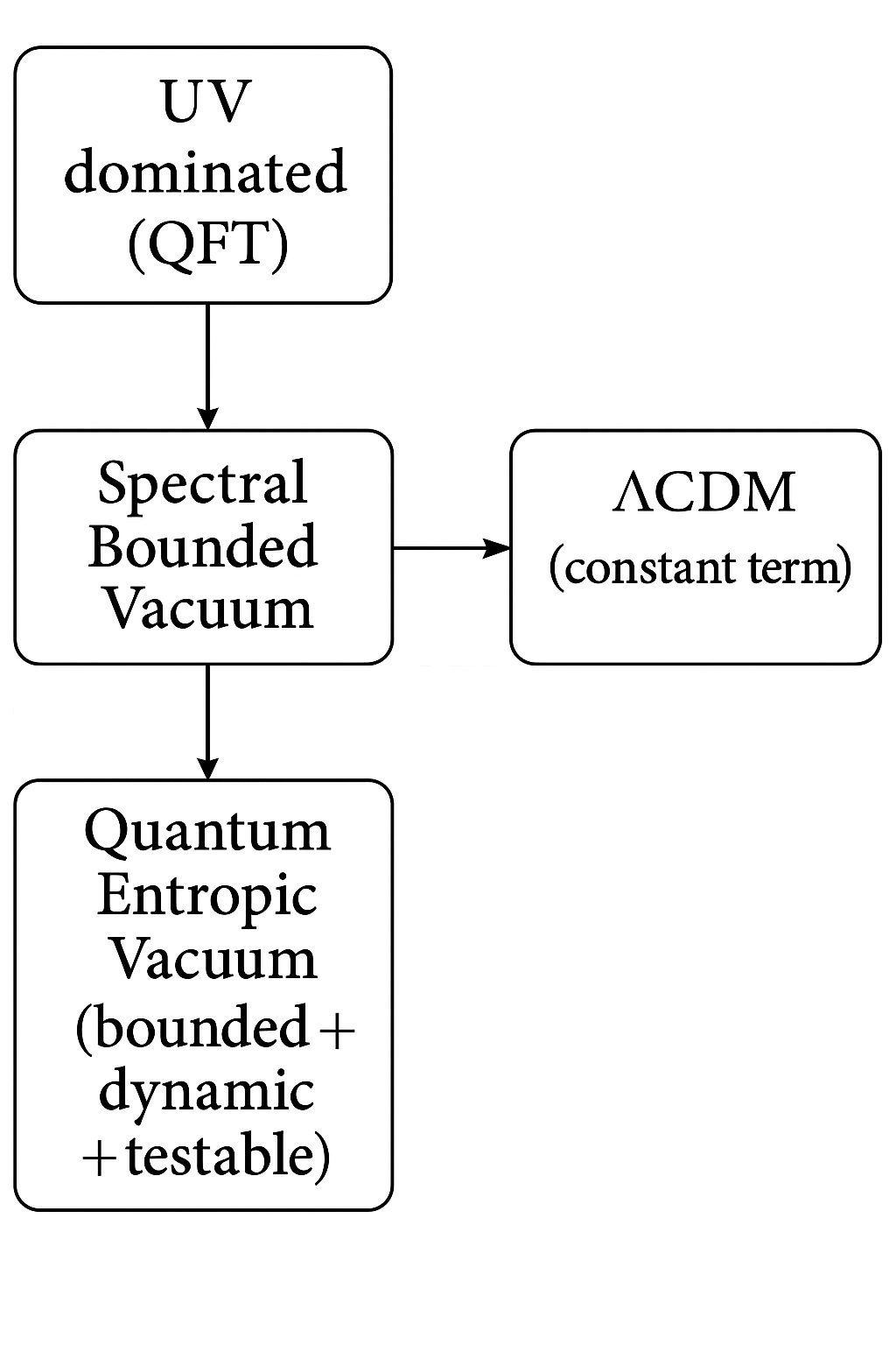
Comparative schematic of vacuum-energy models.
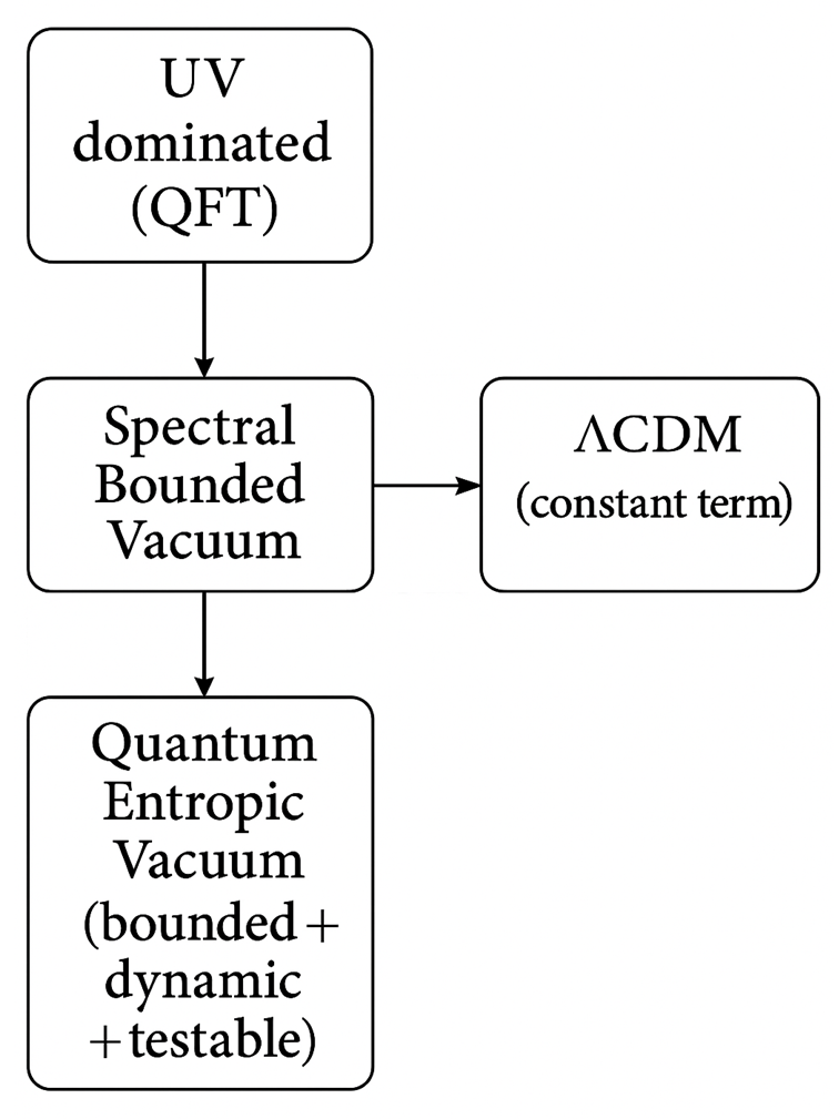
The figure illustrates the conceptual hierarchy among four representative approaches: the UV-dominated quantum field theoretic (QFT) vacuum, the Spectral Bounded Vacuum (SBV) introducing natural UV/IR limits, the Quantum Entropic Vacuum (QEV) as a bounded, dynamic and testable extension, and the conventional CDM model treating as a constant term. Arrows indicate theoretical progression and conceptual refinement, with QEV providing a consistent effective description that remains falsifiable in both cosmological and laboratory contexts.
10. Symbols and Notation
Table 4.
Key symbols used in this work (evaluated at the present epoch unless noted).
| Symbol | Meaning | Units / Value |
|---|---|---|
| Pivot spectral scale today, | ||
| UV bound (hadronic/confinement scale) | 1 (typ.) | |
| IR bound today, | ||
| Effective normalisation today (dimensionless) | – | |
| Net damping/renormalisation today (dimensionless) | – | |
| Present-day vacuum energy density | ||
| C | Kernel constant, | – |
| , | Equation of state (background), | – |
| – | ||
| Deceleration parameter | – | |
| Growth-rate amplitude | – | |
| Late-time IR temperature parameter | ||
| Reduced Planck constant, speed of light, Boltzmann constant | – | |
| Modified Bessel function of the second kind | – | |
| Photonic response window (dimensionless) | – | |
| Band-averaged photonic phase/observable | – | |
| Kernel exponents in the spectral window | – | |
| Kinematic slope parameter (robustness tests) | – | |
| Damping/renormalisation split (gravity / thermal / hadronic) | – | |
| Gravitational projection weight for sector s | – | |
| Sector-specific pivot scale, | ||
| Sector-specific UV bound | ||
| Sector-specific normalisation (dimensionless) | – | |
| Photonic phase/observable at frequency | – | |
| Isotropic SME photon-sector coefficient (mapping reference) | – |
We distinguish a microscopic (pre-damping) and the effective present-day amplitude entering .
11. Conclusion
The cosmological constant can be understood as an emergent macroscopic parameter resulting from the collective dynamics of the quantum vacuum. Within the dynamic QEV model, the vacuum evolves under interacting damping mechanisms that self-regulate its energy density. The residual value observed today represents the asymptotic equilibrium of these processes, a balance between spectral bounding and accumulated gravitational and hadronic attenuation. This formulation unifies micro-physical QCD-scale fluctuations with macroscopic cosmological behavior and offers a consistent, bounded description of vacuum energy without fine-tuning.
Conclusion and Outlook: Decision Points
We have shown that a spectrally bounded vacuum with a single pivot scale L and modest damping can yield the observed late–time acceleration while predicting concrete signatures across scales. To make rapid progress, we suggest a two-pronged test:
- 1.
- Cosmology (12–24 months): Publish a blinded analysis of and where are the reported parameters alongside . A result consistent with and at the percent level would strongly limit the SBV/QEV parameter space.
- 2.
- Laboratory (6–18 months): Perform Casimir/cavity measurements sweeping – mm at controlled temperature to probe the predicted spectral window. A detected, repeatable dispersion/pressure feature near mm would support the framework; a clean null at precision would disfavor its minimal form.
Either outcome is decisive: detection fixes and calibrates the theory; non-detection at the quoted precisions rules out the minimal kernel, motivating either a refined kernel or abandonment of the SBV/QEV explanation.
The results presented here are intended as the foundational component of the broader QEV framework; further unification aspects are deferred to future work building on this structure.
Appendix A. Analytic Integrals
For the hadronic window corresponding to , we define
leading to the mean energy
This yields a typical local contribution within the QEV formalism.
Appendix B. Log-Uniform Weighting
An alternative to the double-exponential damping uses a logarithmic weighting
which provides a simple sensitivity check while preserving the bounded nature of the spectrum.
Appendix C. Numerical Worked Example (Detailed)
Objective. Provide a transparent, reproducible calculation that yields a present-day vacuum energy density close to the observed cosmological constant, (Planck 2018), using the dynamic QEV framework with bounded spectral support and time-dependent damping.
We emphasize that the numerical damping partition shown here represents an integrated historical renormalization from early epochs; in the baseline propagation-only model used for late-time predictions, is not an active dynamical channel.
Appendix C.1. Constants and Late-Time Scales
Define the central window scale
Physical meaning of L.
The quantity represents the characteristic wavelength of the spectral window contributing to the vacuum energy density. It is the geometric mean between the ultraviolet cutoff and the infrared cutoff , and thus marks the midpoint of the logarithmic spectral range. Physically, L acts as an effective coherence length of the quantum vacuum: modes with are suppressed by ultraviolet damping, while modes with are frozen out thermally. The resulting vacuum energy scales as
so that any change in the UV or IR boundaries translates into a quartic variation of . For the fiducial parameters and , the effective scale is , corresponding to the soft X–UV regime.
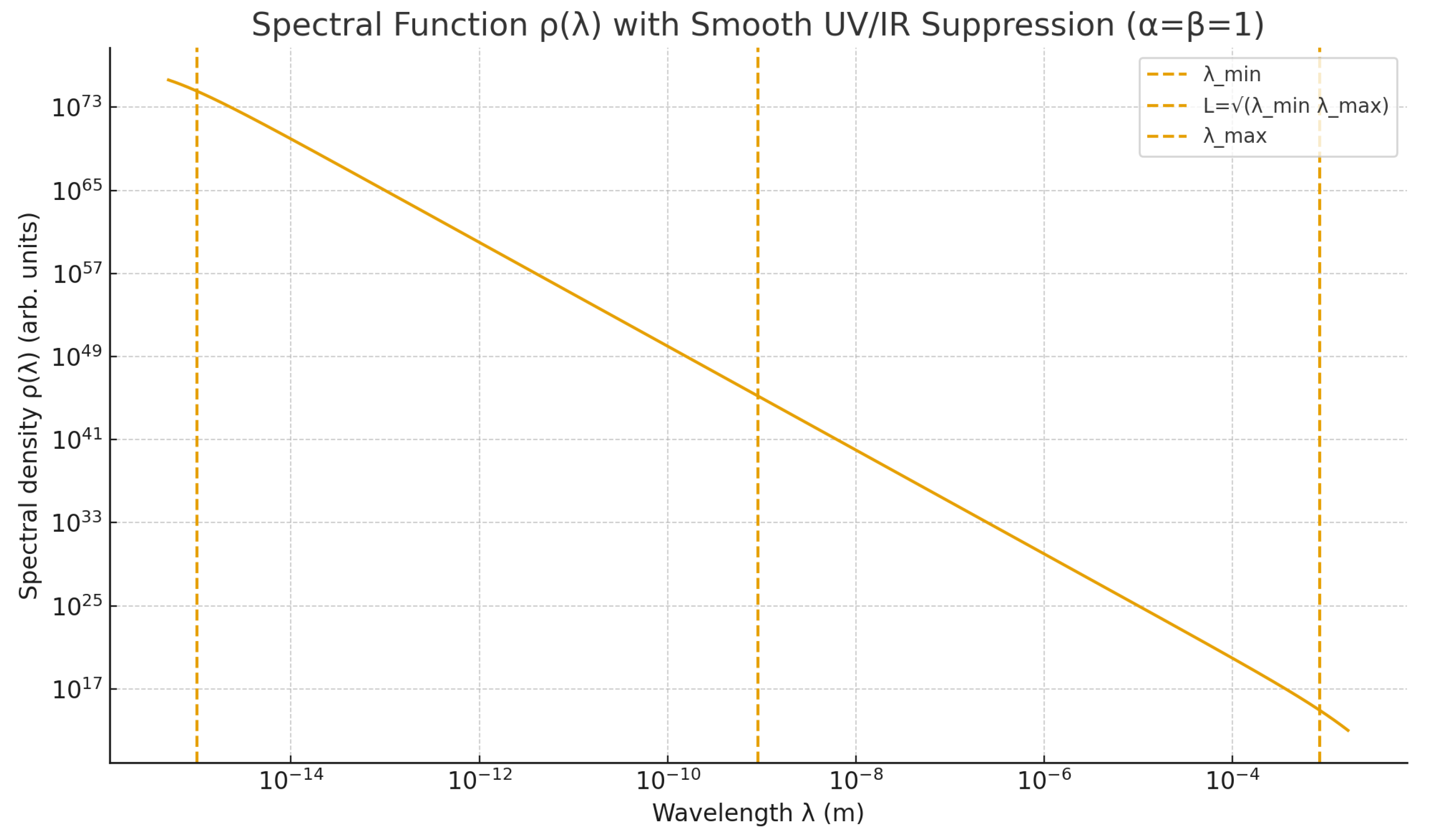
Figure A1.
Spectral function with smooth UV/IR suppression (). Vertical markers indicate fm, , and .
Figure A1.
Spectral function with smooth UV/IR suppression (). Vertical markers indicate fm, , and .
Constants and scales
Table A1.
Physical constants and model scales — cleaned and SI-consistent.
| Symbol | Definition | Value | Units / Notes |
|---|---|---|---|
| h | Planck constant | ||
| Reduced Planck | |||
| c | Speed of light | ||
| Boltzmann constant | |||
| Reference vacuum density | |||
| UV floor (hadronic) | (QCD confinement scale) | ||
| IR temperature scale | |||
| ( ) | |||
| L | ( ) | ||
| C | dimensionless | ||
| Total damping budget | 101 | dimensionless |
Appendix C.2. Spectral Integral with Double-Exponential Kernel
We use the symmetric kernel () and an energy density per wavelength
Then
With ,
Numerically, .
Hence:
Calibration to :
Normalization.
Matching a target value fixes the dimensionless amplitude
Numerical evaluation (fiducial parameters).
We adopt and , so that
For the Bessel factor we use
Naturalness of the normalization constant A0.
The constant represents the microscopic spectral normalization before any macroscopic damping or entropy production. Dimensionally it originates from the mode-counting prefactor in , which for a free relativistic field is naturally of order unity when expressed per helicity state and per spatial dimension. The large effective value inferred from present-day calibration () does not imply fine-tuning but compensates for the cumulative, physically motivated attenuation by the total damping factor . Each partial contribution—gravitational, thermal/entropic, and hadronic—reduces the active spectral weight exponentially over cosmic time; their product yields the minute vacuum density observed today. The resulting ratio
naturally bridges the QCD-scale vacuum and the current cosmological value without requiring delicate cancellations among large ultraviolet contributions. In this sense the QEV model renders the observed vacuum energy technically natural: it emerges from an microscopic amplitude modulated by a physically derived, time-integrated damping history rather than from an ad-hoc balance of divergent terms.
Figure A2.
Double-exponential kernel versus (log–log). Peak scale .
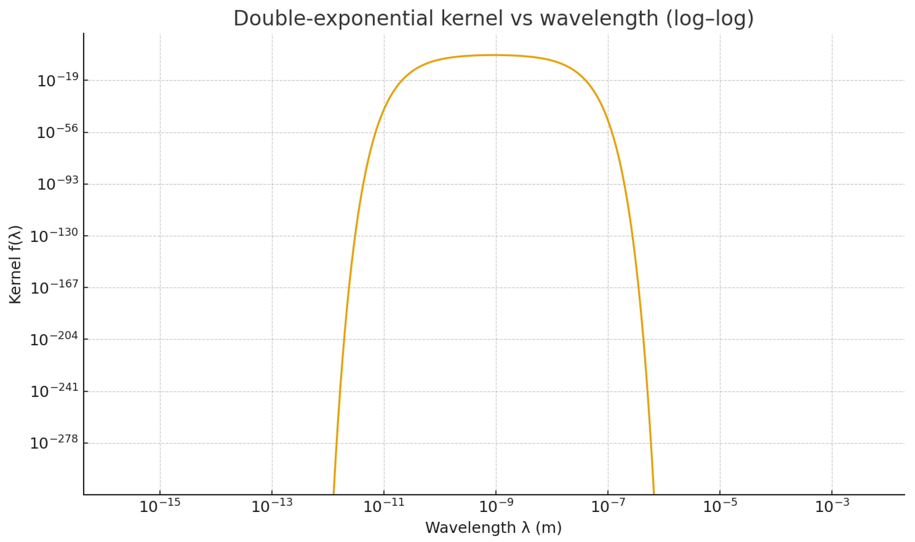
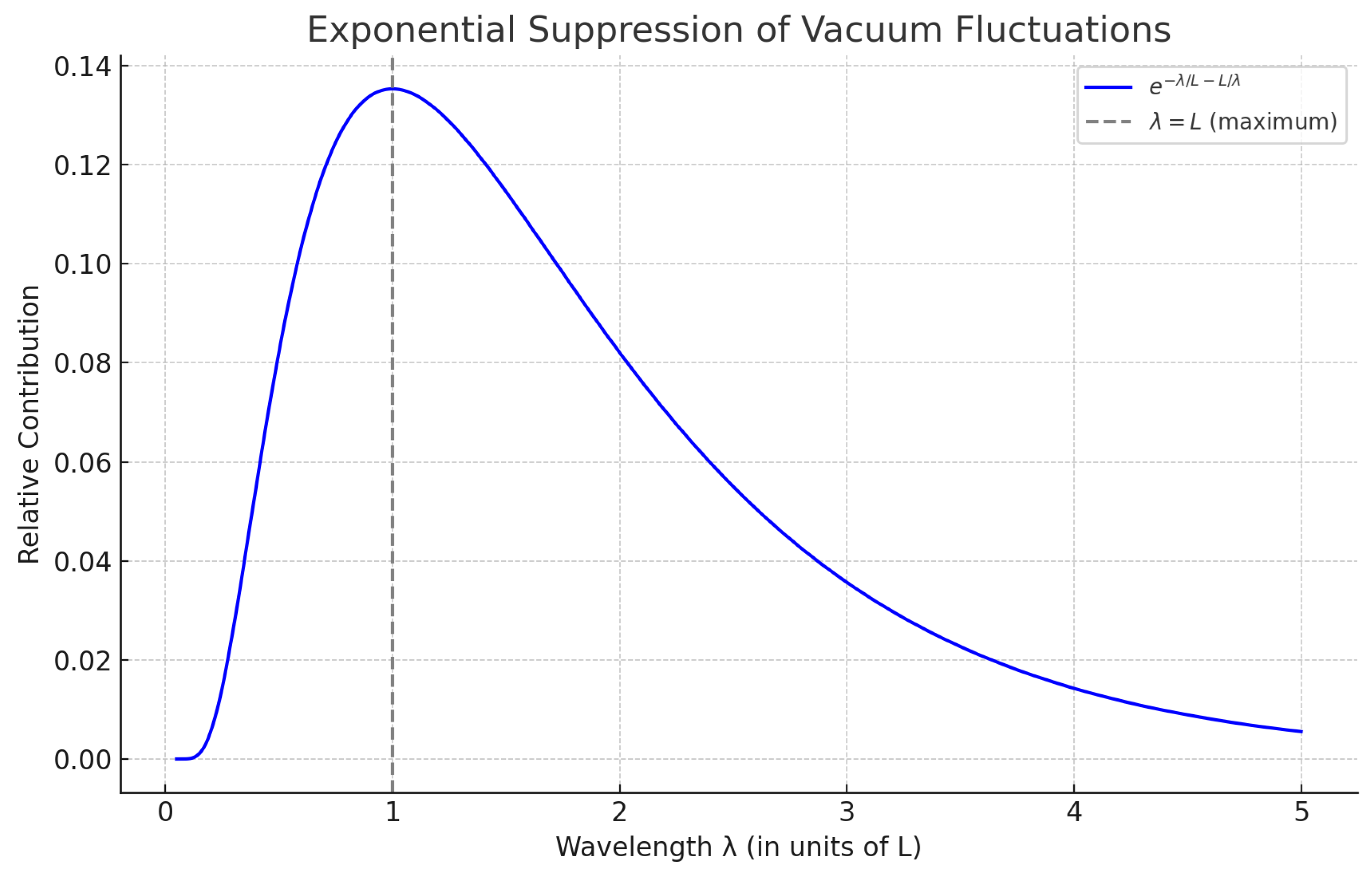
Figure A3.
Exponential suppression of vacuum fluctuations , with a maximum at . This explains why the geometric-mean scale dominates the bounded spectral integral.
Figure A3.
Exponential suppression of vacuum fluctuations , with a maximum at . This explains why the geometric-mean scale dominates the bounded spectral integral.
Relative spectral scaling versus the scaling factor.
Figure A4.
Relative spectral scaling versus the scaling factor.
Trend: .
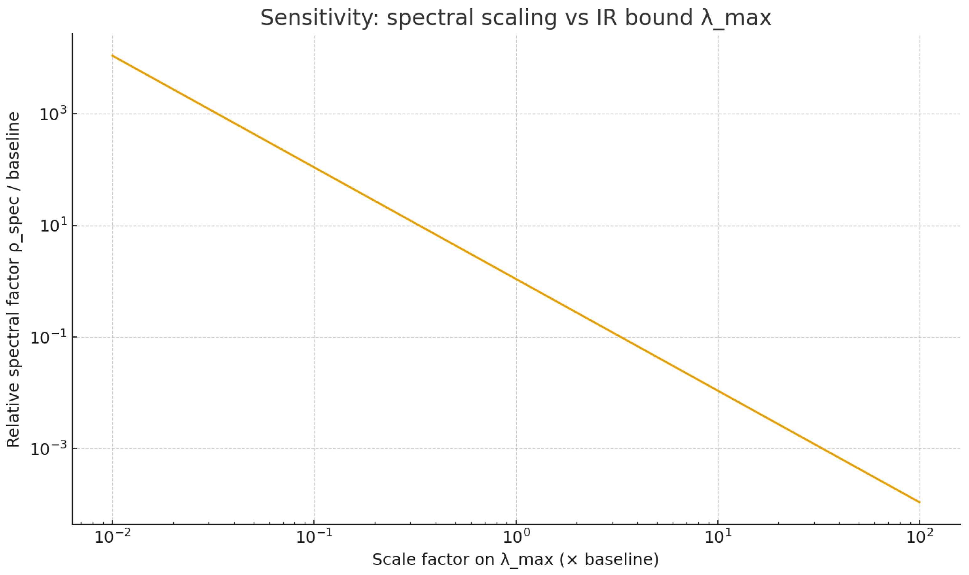
For completeness, we note that for the symmetric kernel used here, the sensitivity with respect to the lower spectral bound behaves identically, yielding . Hence, within the interval , the resulting scaling remains effectively invariant, demonstrating the robustness of the spectral symmetry .
Figure A5.
Spectral function computed from with and . Vertical markers: fm, , . Compare with Fig. Figure A1 (where ).
Figure A5.
Spectral function computed from with and . Vertical markers: fm, , . Compare with Fig. Figure A1 (where ).
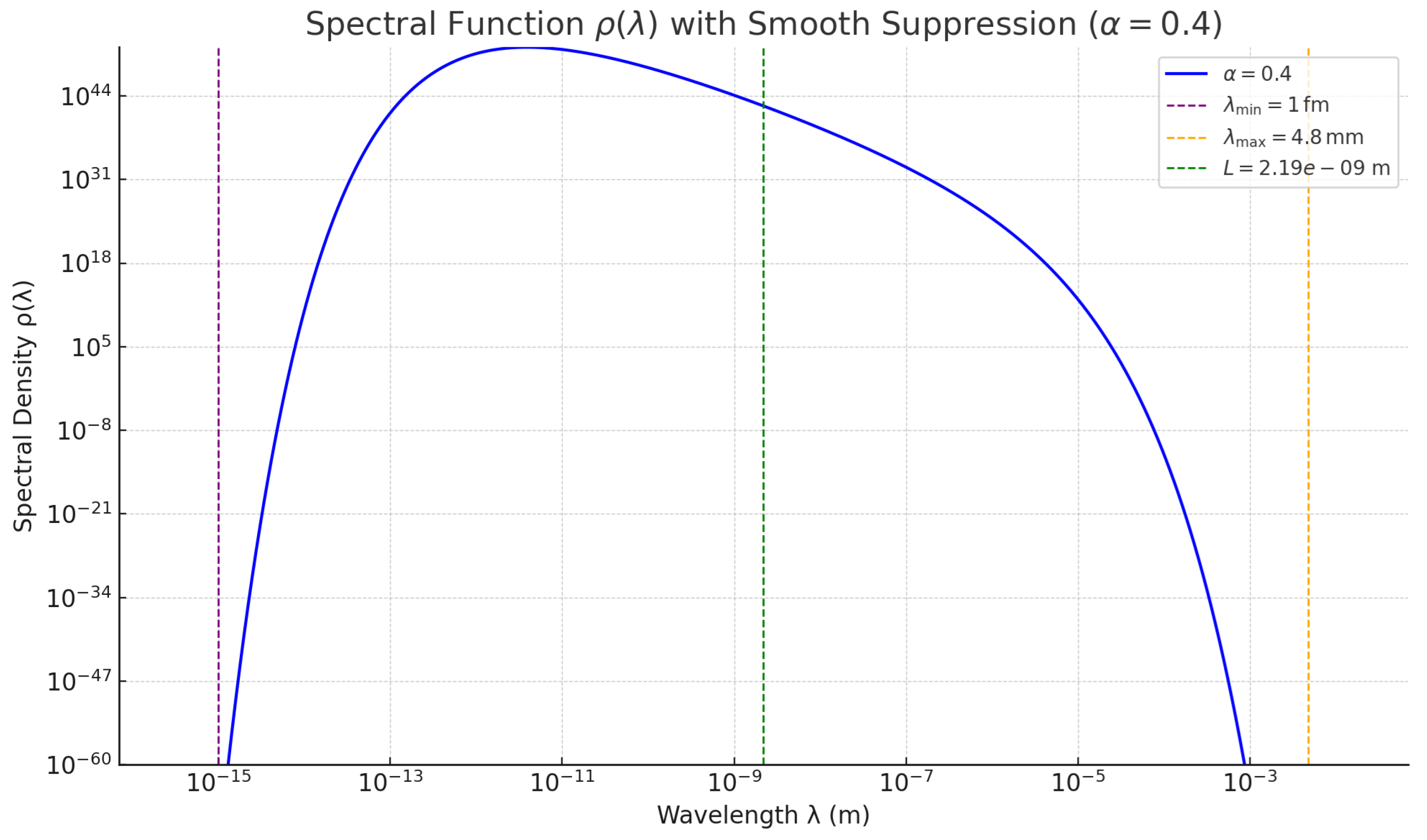
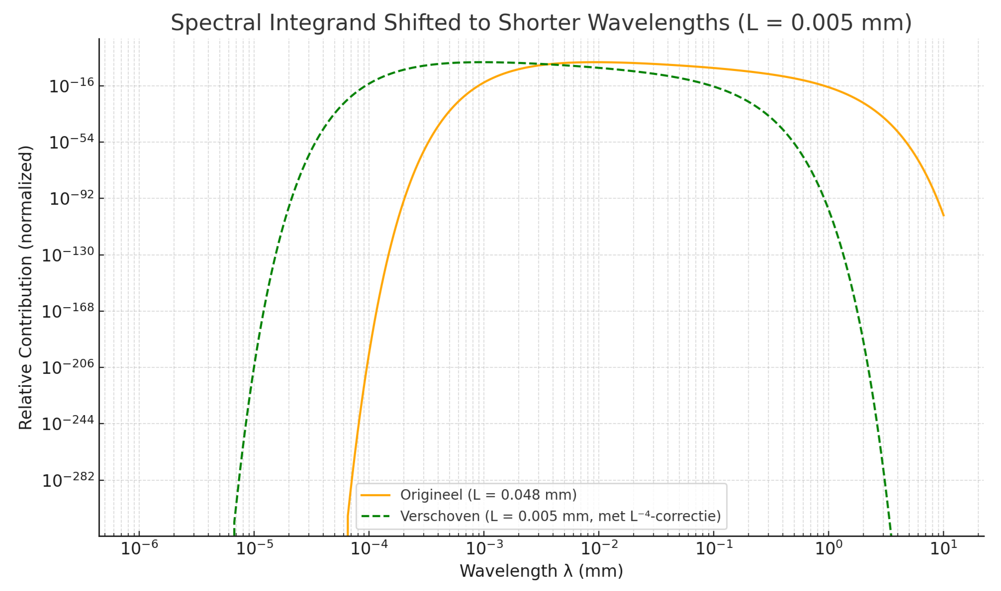
Figure A6.
Evolutionary shift of the effective spectral integrand towards shorter wavelengths as the IR scale tightens (cooling/expansion). The overall scaling follows the normalization.
Figure A6.
Evolutionary shift of the effective spectral integrand towards shorter wavelengths as the IR scale tightens (cooling/expansion). The overall scaling follows the normalization.
Appendix C.3. Dynamic Damping from QCD Scale to Today
The dynamic QEV model couples the bounded spectrum to a damping budget,
with . Taking and fixes the required integrated damping
A representative, physically motivated split is
Here , while collects thermal/entropic suppression (depends on )
and a Gaussian-like peak around .
The damping partition is summarized in Table 3 and visualized in Fig. 7; the IR-driven spectral shift is shown in Fig. 6, while the peak-at-L mechanism is illustrated in Fig. 4.
Figure A7.
Damping budget (pie): , , (total ).
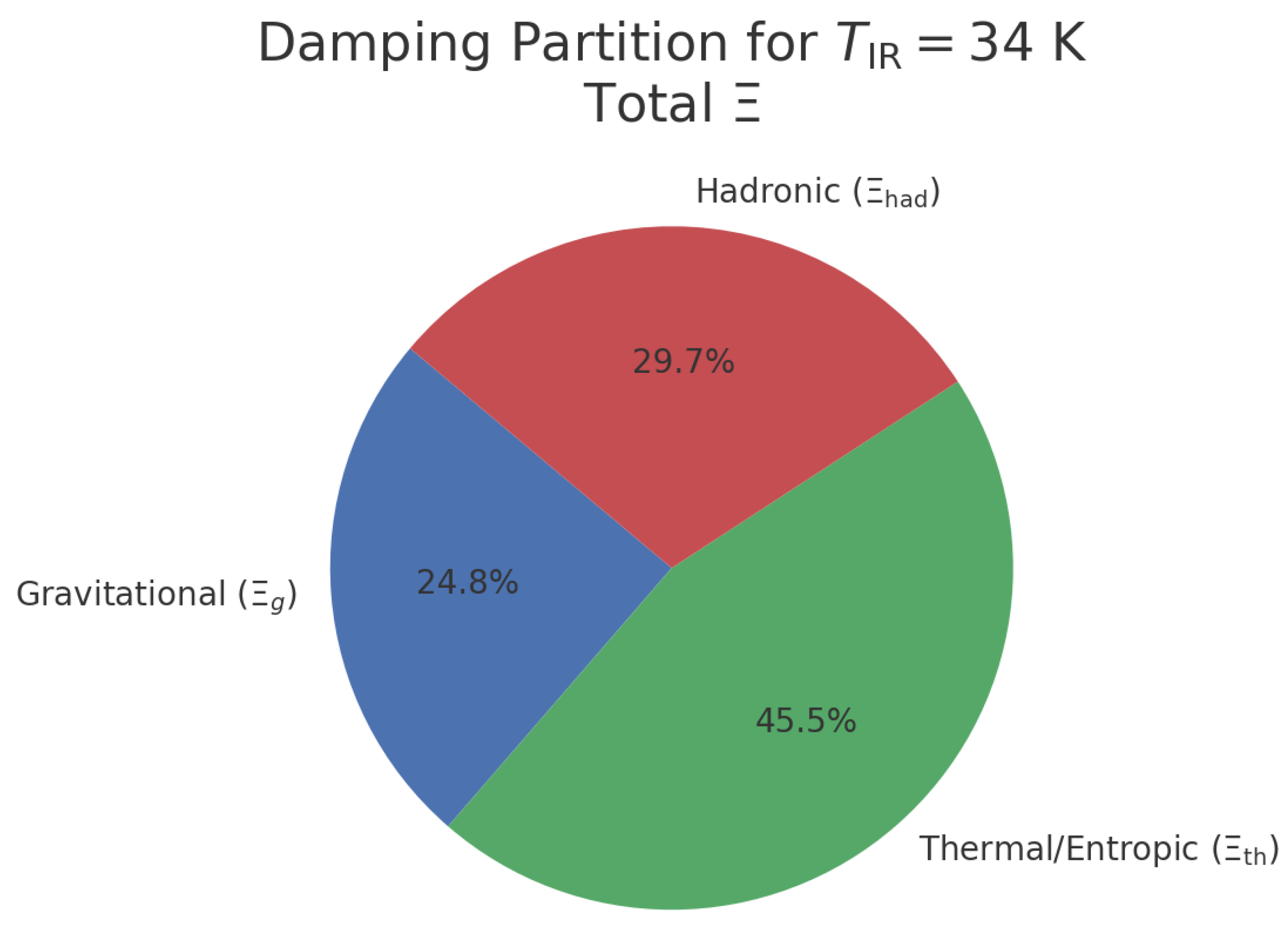
Table A2.
Illustrative damping split to match .
| Component | (e-folds) |
|---|---|
| Gravitational (Hubble) | 25 |
| Thermal/Entropic | 46 |
| Hadronic | 30 |
| Total | 101 |
Appendix C.4. Numerical Plug-In and Result
Combine the spectral factor and damping at :
With and C = 4.3918318548 one finds
Figure 6 explicitly shows how tightening the IR bound shifts the effective integrand to shorter wavelengths; the overall normalization follows the scaling of Eq. (A5)
Appendix C.5. Numerical Plug-In and Result (with Fiducial Scales)
Combine the spectral factor and the dynamic damping at :
Calibrating to gives
which reproduces and, inserted back into Eq. (A6), returns by construction.
Appendix Sensitivity of ρ vac to the Damping Budget Ξ
Fix by calibrating Eq. (A10) at so that today. Then for any other (keeping fixed) the prediction is
Table A3.
Sensitivity of the predicted vacuum energy density to the total damping budget , holding the normalization fixed to its calibration.
Table A3.
Sensitivity of the predicted vacuum energy density to the total damping budget , holding the normalization fixed to its calibration.
| [J ] | ||
|---|---|---|
| 80 | 1.318816e+09 | 7.865024e-01 |
| 90 | 1.784823e+05 | 1.063758e-04 |
| 95 | 1.317006e+03 | 7.847355e-07 |
| 100 | 9.948374e+00 | 5.924162e-09 |
| 101 | 1.000000e+00 | 5.960000e-10 |
| 102 | 1.004987e-01 | 5.929722e-11 |
| 105 | 6.737947e-03 | 4.011837e-12 |
| 110 | 6.737947e-05 | 4.011837e-14 |
Appendix C.6. Conclusion (Concise Summary)
- We model the vacuum as a dynamic, spectrally bounded medium: a UV bound from QCD confinement () and a thermal/entropic IR bound at defining a peak scale L = .
-
With the double–exponential kernel, the late–time spectral contribution is:with
- With the dimensionally-correct form the calibrated normalization reads (e.g. .
- Time–dependent damping encodes gravitational (Hubble), thermal/entropic, and hadronic effects. The required integrated damping to reach today is e–folds, e.g. a representative split , , .
- The calibrated result matches the observed vacuum density: (Planck 2018), with late–time .
- Sensitivities are mild and controlled: at fixed , ; order–unity changes in kernel shape shift by order–unity; .
D. Appendix D. Effective Infrared Scale and Physical Interpretation
Scope and Intent
This appendix clarifies the physical interpretation of the infrared scale used throughout this work. The discussion is intentionally interpretative and does not introduce new assumptions or alter any quantitative results presented in the main text.
We emphasize that is not a critical temperature of the quantum vacuum and does not correspond to a physical phase transition, symmetry breaking, or change in the fundamental interactions of matter. All late-time predictions of the SBV/QEV framework follow from the effective spectral window evaluated at the present epoch and do not rely on a literal transition at .
Thermal Structuring and Spectral Selection
In a universe containing stable matter, chemistry, and macroscopic structure, temperature acts as a selection mechanism rather than a constitutive property. Physical structures exist only within temperature ranges where thermal agitation does not destroy binding or coherence. This principle applies equally to the long-wavelength sector of vacuum fluctuations.
Accordingly, the infrared scale should be understood as an effective reference scale characterizing the regime in which thermally populated long-wavelength modes become negligible compared to quantum ground-state fluctuations. Below this scale, thermal noise no longer masks the infrared vacuum contribution, and the gravitationally relevant part of the spectrum stabilizes.
Relation to the Spectral Window
The effective infrared wavelength
parametrizes the longest vacuum modes that remain physically meaningful within a thermally structured universe. This scale does not represent a hard cutoff but rather a smooth, context-dependent boundary defining the infrared extent of the spectral window.
Once the universe cools into the late-time regime (), variations in become slow and logarithmic, leading to an approximately constant geometric mean scale
and hence to a stable vacuum energy density .
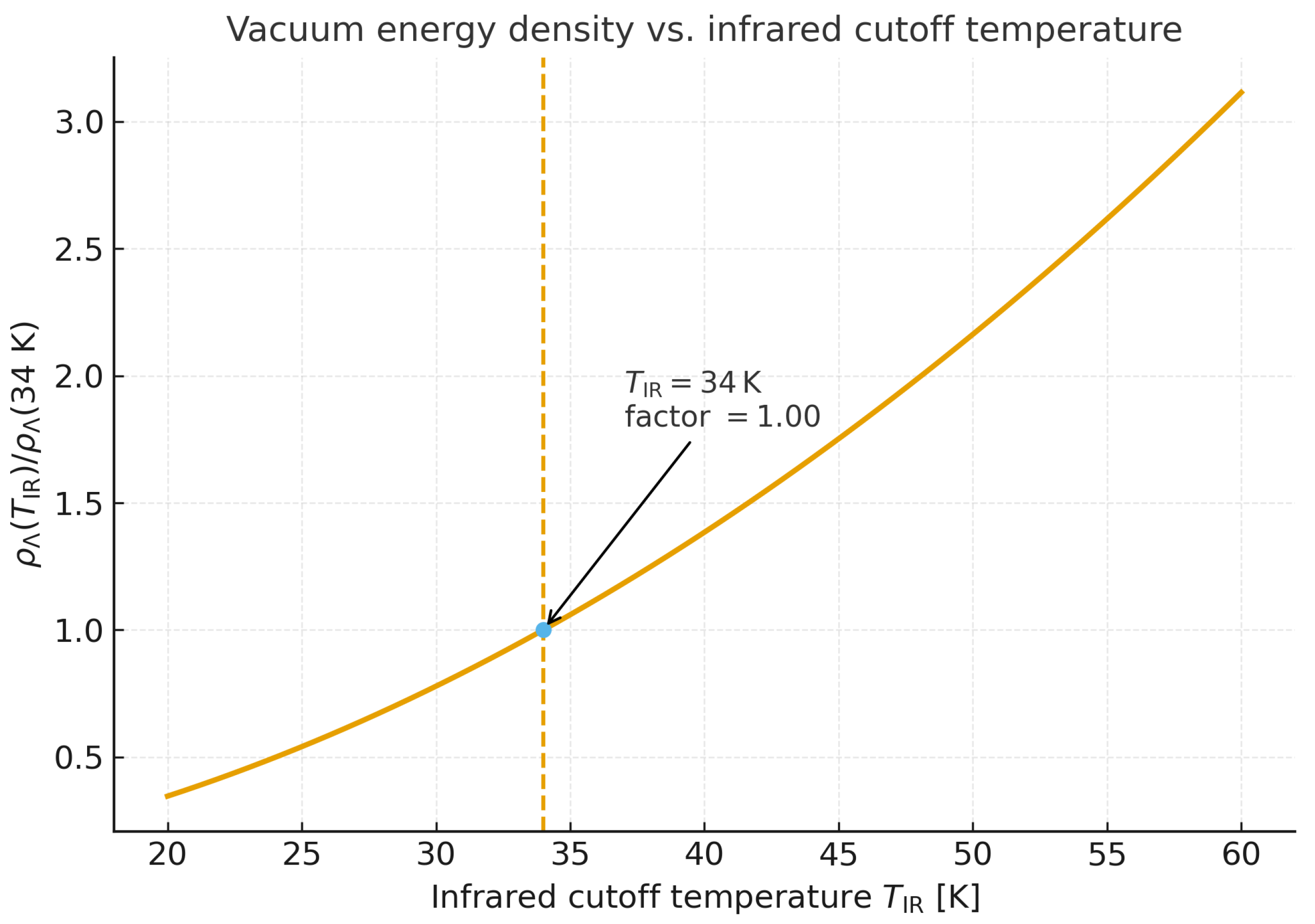
D.1. Visual Representation of the Infrared Sensitivity
Figure A8.
Dependence of the normalized vacuum energy density on the infrared cutoff temperature in the range 20–. The dashed line indicates a representative infrared reference scale; it does not correspond to a physical phase transition of the vacuum.
Figure A8.
Dependence of the normalized vacuum energy density on the infrared cutoff temperature in the range 20–. The dashed line indicates a representative infrared reference scale; it does not correspond to a physical phase transition of the vacuum.
D.2. Broader Implications
The coincidence between the energy scale and characteristic condensation energies in condensed-matter systems is suggestive, but should be interpreted with care. In the present framework, does not represent a critical temperature of the vacuum, but an effective reference scale associated with the late-time thermal structuring of the universe. See Fig. Figure A8.
Any analogy to macroscopic coherence phenomena is therefore heuristic rather than literal: it highlights the role of temperature in selecting which long-wavelength modes remain physically relevant, without implying a phase transition or symmetry breaking of the vacuum.
Appendix E. Effective Fluid Formulation of the QEV Vacuum
...
The Quantum Entropic Vacuum (QEV) energy density can be cast as an effective cosmological fluid in the Friedmann–Robertson–Walker (FRW) background, allowing explicit verification of energy–momentum conservation and of the asymptotic equation-of-state .
Appendix E.1. Energy–Momentum Conservation
In a homogeneous and isotropic Universe the conservation law
reduces to the continuity equation
where is the Hubble rate. The QEV energy density follows from the spectral-bounded ansatz
with fixed by confinement physics and tracing the evolving infrared limit.
Differentiating Eq. (A12) yields
Substitution into Eq. (A11) gives the effective pressure
Hence the instantaneous equation-of-state parameter is
When becomes constant—as expected after the thermal/entropic freeze-out—one obtains and , recovering the cosmological-constant limit.
Appendix E.2. Example Scaling of L(a)
If the infrared cutoff evolves with temperature as while remains fixed, then and
corresponding to a transient radiation-like phase that is exponentially damped once the entropic factor saturates. In the late-time regime of interest, stabilises and within deviations .
Appendix E.3. Sound Speed and Stability
Perturbing Eq. (A11) at constant entropy gives the adiabatic sound speed
For monotonic with slowly varying slope, the correction term is small and . This implies a non-propagating (quasi-vacuum) mode with no ghost or gradient instability in the FRW background.
-
Appendix E.11.11.18. Perturbations and closure.
The adiabatic derivative of the effective-fluid relations yields . We emphasize that the QEV component is a quasi-vacuum sector with non-propagating rest-frame fluctuations; in practice we adopt a non-adiabatic (rest-frame) closure so that no rapid gradient instabilities arise in large-scale-structure regimes. Linear-growth observables are evaluated in the background limit with the baseline (propagation-only) choice, which is sufficient for the percent-level deviations reported here.
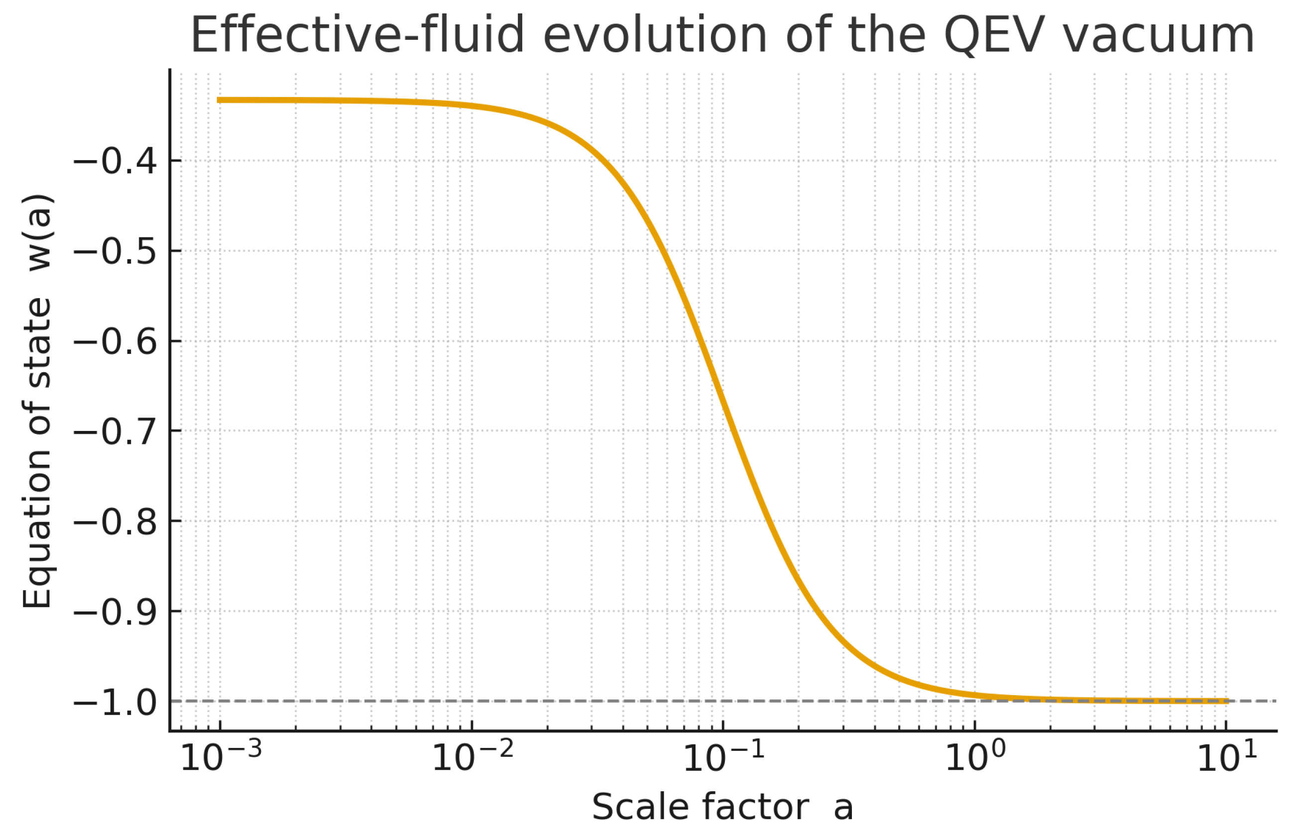
Figure A9.
Effective-fluid evolution of the QEV vacuum. The equation of state follows . The illustrative curve uses a smooth early-to-late transition with , yielding a radiation-like phase ( for ) that relaxes toward a cosmological-constant limit () once saturates (). At late times the deviation is small, for the example shown.
Appendix E.4. Summary
The effective-fluid form Eqs. (A13)–(A14) guarantees by construction. The model evolves smoothly from a damped, radiation-like early stage ( to ) toward a late-time cosmological-constant state (), maintaining stability and internal energy conservation. This demonstrates that the QEV vacuum is formally covariant and self-consistent at the effective-fluid level.
Appendix F. Thermal Route: Baseline Choice and Variants
Appendix F.12.12.19. Baseline (Propagation-Only) Model.
To avoid double counting of thermal/entropic physics, we define the baseline QEV model by encoding all thermal effects exclusively in the infrared propagation cutoff and setting explicit thermal source damping to zero:
with the cosmological radiation temperature including the usual entropy–dilution factor, .1
Notation: . The QEV energy density remains
At late times freezes (or varies only logarithmically), so and L approach constants and .
Appendix F.12.12.20. Rationale.
All thermal dependence is carried by propagation (the spectral window). No additional exponential suppression is applied to the source side:
This makes the mapping from temperature to observables one-to-one and prevents thermal physics from being counted twice (both in and in an extra damping factor).
Appendix F.12.12.21. Implementation notes.
- Use . Across known transitions (QCD, annihilation), update piecewise-constantly.
- Keep fixed (QCD floor). Then and .
- Late-time fits (SNe+BAO+CC): treat as parameters, with the freeze-out scale where saturates.
Appendix F.12.12.22. Optional Variant (Source-Only Thermal Damping).
For comparison studies one may switch off thermal propagation evolution and encode thermal effects purely as source damping:
with a single calibrated history (e.g. smooth step across known thermal epochs). In this variant, do not allow T-dependence in . Then and by construction; thermal impact enters only via the normalization .
Appendix F.12.12.23. No double counting (rule of thumb).
Appendix F.12.12.24. Parameter priors (recommended).
These priors reflect percent-level kinematic robustness and keep the baseline identifiable.
Appendix F.12.12.25. Reporting.
Clearly state the chosen route in captions/tables: “Baseline (propagation-only)” or “Variant (source-only)”. Quote at and the mm-band target observable (e.g. cavity phase or Casimir window) using the same choice.
Appendix G. Response to Scope Critique (Early-Universe Comparison)
Our model is a late-time effective description: we evaluate the spectral, gravitationally relevant contribution at the present epoch . We make no claim about the absolute zero-point energy of the early Universe or about inflation. Historical processes are summarised by a convergent damping factor that we do not attempt to reconstruct at high temperatures. All equations and predictions are restricted to low redshift (), where direct falsification is possible through background and growth measurements, and through tabletop tests in the millimetre band.
References
- P. A. Abell et al., LSST Science Book, Version 2.0 (2009). arXiv: 0912.0201.
- P. Ade et al., The Simons Observatory: Science goals and forecasts, JCAP 02, 056 (2019). arXiv: 1808.07445. [CrossRef]
- P. Ade et al., The Simons Observatory: Science Goals and Forecasts for the Large Aperture Telescope (2025). arXiv: 2503.00636.
- Birrell, N. D.; Davies, P. C. W. Quantum Fields in Curved Space; Cambridge University Press, 1982. [Google Scholar]
- Euclid Collaboration (A. Blanchard et al.), Euclid preparation: VII. Forecast validation for Euclid cosmological probes (2019). arXiv: 1910.09273.
- H. B. Callen, Thermodynamics and an Introduction to Thermostatistics, Wiley (1985).
- Colladay, D.; Kostelecký, V. A. Lorentz-violating extension of the standard model . Phys. Rev. D arXiv: hep-ph/9809521. 1998, 58, 116002. [Google Scholar] [CrossRef]
- Euclid Collaboration (J.-C. Cuillandre et al.), Euclid: Early Release Observations (ERO): Perseus Cluster (2024). arXiv: 2405.13501.
- Dhital, M.; Mohideen, U. A Brief Review of Some Recent Precision Casimir Force Measurements . Physics 2024, 6(2), 891–904. [Google Scholar] [CrossRef]
- Elsaka, B.; Sedmik, R. I. P. Casimir Effect in MEMS: Materials, Geometries, and Metrologies—A Review . Micromachines 2024, 15(6), 1202. [Google Scholar] [CrossRef] [PubMed]
- L. Freidel, F. Hopfmueller, and E. R. Livine, Gravitational Energy, Local Holography and Entanglement in Gravity, Class. Quantum Grav. 40, 085005 (2023), arXiv:2212.07382 [gr-qc].
- L. Freidel, J. Kowalski-Glikman, R. G. Leigh, and D. Minic, "Vacuum Energy Density and Gravitational Entropy," Phys. Rev. D 107, 126016 (2023). arXiv: 2212.00901.
- A. J. H. Kamminga, "Vacuum Density and Cosmic Expansion: A Physical Model for Vacuum Energy, Galactic Dynamics and Entropy" (2025). [CrossRef]
- A. J. H. Kamminga, “Photonic Vacuum Windows: A Casimir-Safe Operational Baseline” (2025). [CrossRef]
- J. I. Kapusta and C. Gale, Finite-Temperature Field Theory: Principles and Applications, Cambridge University Press (2006).
- F. R. Klinkhamer and M. Risse, "Vacuum energy density from a spectral cutoff," arXiv: 2102.11202 [gr-qc] (2021).
- Klinkhamer, F. R.; Schreck, M. Improved bound on isotropic Lorentz violation in the photon sector . Phys. Rev. D 2017, 96, 116011. [Google Scholar] [CrossRef]
- Martin, J. Everything you always wanted to know about the cosmological constant problem (but were afraid to ask) . C. R. Physique 1205.3365. 2012, 13(6–7), 566–665. [Google Scholar] [CrossRef]
- H. M. Nussenzveig, Causality and Dispersion Relations, Academic Press (1972).
- F. W. J. Olver, D. W. Lozier, R. F. Boisvert, and C. W. Clark (eds.), NIST Digital Library of Mathematical Functions, Chap. 10: Bessel and Modified Bessel Functions (2025). https://dlmf.nist.gov/10.
- Planck Collaboration. Planck 2018 results. VI. Cosmological parameters. Astron. Astrophys. 2020, 641, A6. [Google Scholar] [CrossRef]
- Weinberg, S. The cosmological constant problem . Rev. Mod. Phys. 1989, 61, 1–23. [Google Scholar] [CrossRef]
- K. Yagi, T. Hatsuda and Y. Miake, Quark-Gluon Plasma: From Big Bang to Little Bang, Cambridge University Press (2005).
- W. van der Schee, Gravitational collisions and the quark-gluon plasma, PhD thesis, Utrecht University (2014). arXiv: 1407.1849.
- DESI Collaboration (A. G. Adame et al.), DESI 2024 VI: Cosmological Constraints from the First Two Years (2024). arXiv: 2404.03002.
- DESI Collaboration (A. G. Adame et al.), DESI 2024 V: Full-Shape Galaxy Clustering from the First Year of DESI (2024). arXiv: 2411.12021.
| 1 | We use for entropy degrees of freedom and for energy degrees of freedom. |
Disclaimer/Publisher’s Note: The statements, opinions and data contained in all publications are solely those of the individual author(s) and contributor(s) and not of MDPI and/or the editor(s). MDPI and/or the editor(s) disclaim responsibility for any injury to people or property resulting from any ideas, methods, instructions or products referred to in the content. |
© 2026 by the authors. Licensee MDPI, Basel, Switzerland. This article is an open access article distributed under the terms and conditions of the Creative Commons Attribution (CC BY) license (http://creativecommons.org/licenses/by/4.0/).
Copyright: This open access article is published under a Creative Commons CC BY 4.0 license, which permit the free download, distribution, and reuse, provided that the author and preprint are cited in any reuse.


