Submitted:
30 June 2025
Posted:
02 July 2025
You are already at the latest version
Abstract
Zero-day attacks pose substantial risks to cybersecurity by exploiting undetected flaws. Traditional signature-based methods are unable to detect them. The complexities of conventional methods for problem identification exacerbate the dilemma. This study examines diverse approaches for automated identification of computer network and operating system problems, including zero-day vulnerabilities. Techniques encompass Random Forest, One-Class SVM, Naive Bayes, LSTM, BiLSTM, and GRU. We employed a dataset of synthetic network traffic comprising 1,000,000 records and 11 unique attributes. The data include source and destination IP addresses, ports, protocol types, packet and byte transfer metrics, connection length, and attack classifications (IsAnomaly). Before utilising the dataset, it was subjected to multiple processes, including data purification, feature encoding, normalising by StandardAero, and partitioning into training (80%) and testing (20%) subsets. We evaluated the proposed methodology using standard metrics, including accuracy, precision, recall, F1-score, training time, and detection time. The results demonstrated that Random Forest achieved the best overall accuracy (92.4%) and proved to be cost-effective, making it suitable for real-time applications. In contrast, deep learning methodologies achieved a similar performance (about 91%), while necessitating significantly more processing resources. One-Class SVM exhibited its ability to detect anomalies that had not been previously found during attacks. The results demonstrate that systems identifying zero-day threats must strike a balance between speed and precision. This capability enables the creation of more resilient and scalable frameworks.
Keywords:
zero-day attack detection
; machine learning
; deep learning
; computational efficiency
; anomaly-based detection
1. Introduction
Background
Cyber threats are becoming complex, especially zero-day attacks; therefore, we need improved methods for their detection that balance accuracy and speed [1]. Traditional signature-based solutions are ineffective because they depend on recognised attack patterns, enabling new threats to evade detection. Recent advances in machine learning (ML) and deep learning (DL) show promise as alternatives by analysing patterns in network traffic and other data sources [3]. This study explores automatic detection strategies using training datasets to effectively identify and mitigate zero-day threats.
We utilised a synthetic network traffic dataset comprising 1,000,000 records and 11 attributes. These included:
- Source and destination IP addresses indicate where communication begins and ends.
- Source/Destination Ports: This indicates the services or applications utilised.
- Protocol Type: This indicates the specific communication protocols to utilise (such as TCP or UDP).
- Packet/Byte Transfer Statistics: This illustrates the flow of data.
- Duration: The length of time connections last.
- Attack Labels (IsAnomaly) denote whether the traffic is categorised as usual (0) or as an attack (1) [4].
A primary goal is to evaluate the effectiveness of standard and deep learning (DL) models in identifying zero-day attacks.
Two. Evaluating the performance of models regarding efficiency and scalability.
Three. Demonstrating the application of real-time threat detection into cybersecurity frameworks [7].
2. Associated Literature
The research in Table 1 offers insights into different methods for detecting zero-day attacks, emphasising their unique strengths and weaknesses. Ceponis and Goranin (2019) demonstrated the effectiveness of deep learning in system call classification, achieving excellent accuracy on AWSCTD. However, their technology faced scalability challenges, which limited its use in large network environments. Kalash et al. (2020) attained an accuracy of 99.24% in CNN-based malware classification; nonetheless, their approach required extensive labelled datasets, which are often unavailable for zero-day threats.
Gyamfi et al. (2023) used a Single Layer Feedforward Network (SLFN) for anomaly detection in mobile networks, achieving an accuracy of 96.8%. However, their findings were limited to specific datasets, reducing their applicability to wider cybersecurity scenarios. Yuan et al. (2019) introduced the signal-to-noise ratio (SNR) in deep metric learning as a powerful method for optimising distance metrics; yet, its application in cybersecurity remains unexplored. Ding et al. (2022) employed ensemble learning techniques for malware detection, reaching an accuracy between 97.3% and 99%. The study noted a higher false positive rate, despite robust classification accuracy, which could affect real-world implementation.
The results highlight the ongoing challenge of balancing accuracy, computing efficiency, and scalability when identifying zero-day attacks. Deep learning models demonstrate high accuracy; however, their dependence on large volumes of labelled data and significant computing resources limits their application. This study aims to address these issues by assessing both classical and deep learning models using multiple performance indicators, considering real-time usability and computational constraints. Conventional metrics mainly evaluate classification performance; however, the signal-to-noise ratio (SNR) combines accuracy, precision, recall, and computational efficiency into a single composite metric [17]. Yet, researchers have not extensively explored its application in zero-day attack detection.

3. Methodology
3.1. Data Acquisition Procedures
This research relies on a comprehensive synthetic network traffic dataset, specifically selected or created to evaluate the effectiveness of zero-day attack detection. The dataset contains 1,000,000 individual records, each representing a network connection or flow.
The dataset was designed to incorporate 11 essential criteria for differentiating between benign and malicious network activity. These attributes include
Source and Destination IP Addresses
Source and Destination Ports
Protocol Type (e.g., TCP, UDP, ICMP)
Packet and Byte Transmission Metrics
Duration of Connection
A ground truth label ('IsAnomaly') categorises each record as either regular traffic (0) or an assault (1) [4].
This dataset was obtained through a publicly accessible research resource, using the Ostinato traffic generator or simulation tools designed to replicate network attacks; please specify the source or method. This extensive synthetic dataset enables controlled experiments and thorough evaluation of the proposed machine learning and deep learning models in a challenging environment that closely resembles real-world networks facing new threats. After acquisition, the data was organised for analysis as described in the preprocessing phase (phase 3.1).
3.2. Dataset Compilation
The network traffic dataset comprises 1,000,000 records with 11 features, summarised as follows [18].
Illustration 1. Proposed framework
Figure 1.
Proposed framework.
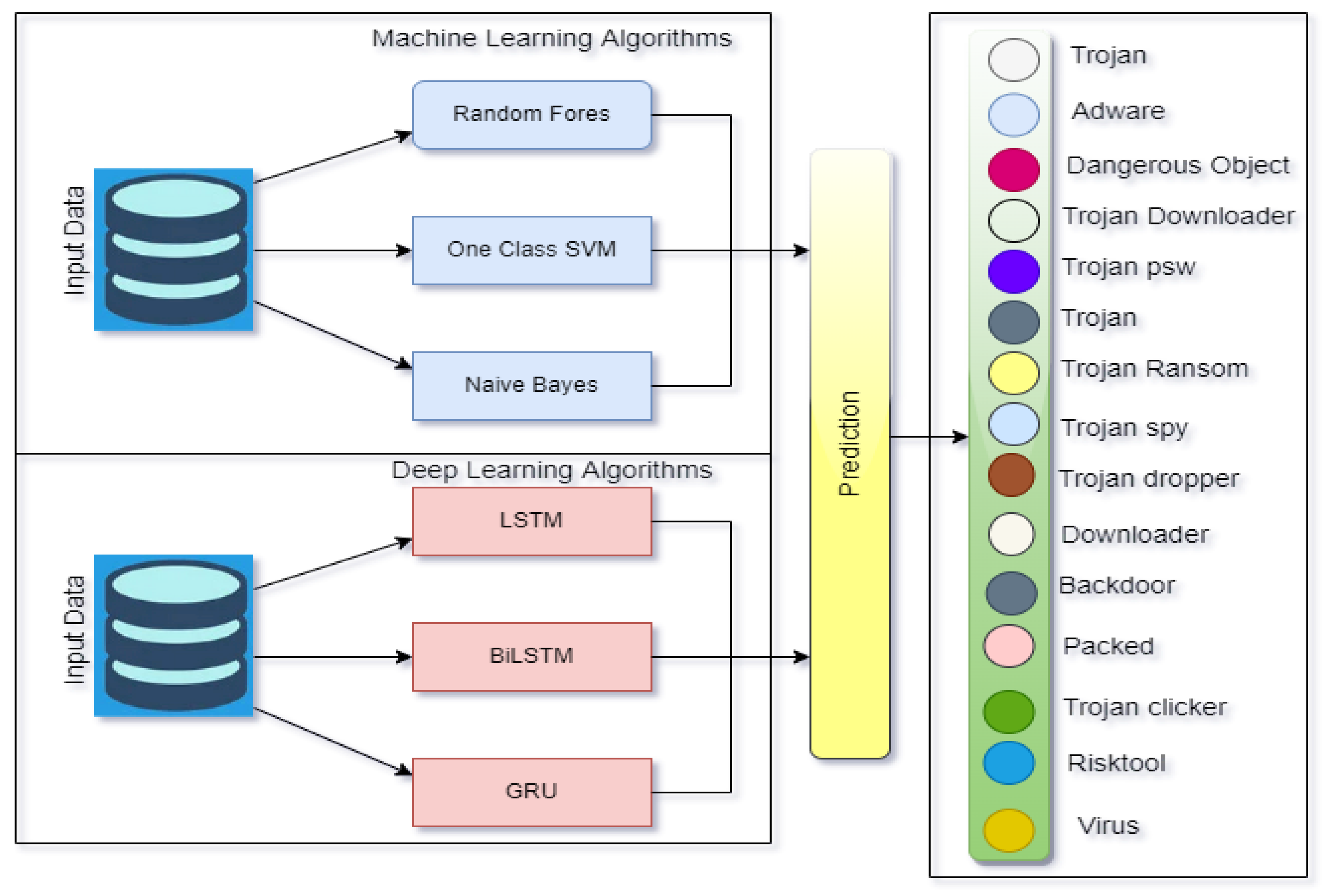
Table 3 offers a detailed analysis of the dataset used in the study. The "Feature" column lists each attribute present in the dataset. "Description" explains the importance of each feature in the context of network traffic analysis. "Data Type" shows whether the feature is numerical (continuous or discrete) or categorical. "Range/Values" indicates the possible values or spectrum of values each feature can take. Notably, "Preprocessing Steps" describes the data modifications applied to each feature, ensuring transparency and reproducibility. This section also details the encoding techniques for categorical variables (e.g., one-hot encoding, hashing) and the scaling methods for numerical features (e.g., StandardScaler, Min-Max Scaling). Such specificity is crucial for other researchers seeking to replicate or extend this study.
The preprocessing procedures encompassed:
Data Cleaning: Eliminated absent or inconsistent values.
Feature Encoding: Transformed categorical features (e.g., protocol type) into numerical representations.
Feature Scaling: Utilised StandardScaler for normalisation.
Data Partitioning: The dataset was grouped into training (80%) and testing (20%) sections [28].
3.3. Executed Algorithms
Table 4 outlines the hyperparameter optimisation process for each model. The "Model" column specifies the particular algorithm. "Hyperparameter" lists the hyperparameters that were optimised for the model. "Search Space" describes the range of values tested for each hyperparameter. "Tuning Method" indicates the search strategy used (e.g., grid search, random search, or Bayesian optimisation). Ultimately, "Best Value" represents the optimal hyperparameter value found through the tuning process, which was then used to train the final model. This table enhances the clarity of the experimental methods and aids other researchers in replicating the study. Including the exact optimisers and learning rates for the deep learning models is crucial for comprehensive understanding.
Six algorithms were implemented to evaluate different detection techniques.
3.4. Assessment Criteria
We assessed the efficacy of the deployed models utilising conventional classification metrics. These measurements depend on the principles of true positives (TP), true negatives (TN), false positives (FP), and false negatives (FN). Within the framework of this research:
§ True Positive (TP): A case accurately recognised as an attack (anomaly).
§ True Negative (TN): A case accurately recognised as standard traffic.
§ False Positive (FP): A case of legitimate traffic erroneously classified as an attack (Type I Error).
§ False Negative (FN): A case of an assault erroneously classified as regular traffic (Type II Error).
We assessed the model's performance with the metrics outlined in Figure 2:
Accuracy: Denotes the overall ratio of correct predictions (including assaults and regular traffic) relative to the total number of incidents. It comprehensively evaluates the model's accuracy (Eqn. 1).
Precision measures the ratio of actual positive cases correctly identified as assaults to the total number of cases predicted as attacks (TP / (TP + FP)). High precision indicates a low rate of false alarms (Eqn. 2).
Recall (Sensitivity or True Positive Rate): Measures the proportion of actual attack occurrences correctly identified by the model (TP / (TP + FN)). A high recall indicates that the model effectively detects most attacks (Eqn. 3).
The F1-score is the harmonic mean of precision and recall, offering a single statistic that balances both. It is particularly useful with imbalanced datasets, as accuracy alone can be misleading (Eqn. 4).
This study aims to identify models that balance high accuracy with computational efficiency for practical deployment. Conventional machine learning models, such as Random Forest and Naive Bayes, offer faster detection times, whereas deep learning models, including LSTM, BiLSTM, and GRU, achieve similar accuracy but demand greater processing resources. This evaluation method allows for a thorough examination of detection models, enabling the selection of optimal solutions that improve.
Both detection efficacy and efficiency are essential in real-time cybersecurity applications.
4. Experimental Configuration
4.1. Characteristics of the Dataset
We conducted preprocessing of the dataset as follows:
Normalisation: Adjusted features to guarantee uniform scaling.
SMOTE: Equalised classrooms to address disparities.
Tokenisation: Transformed sequences into subword units for transformers (if relevant).
4.2. Optimisation of Hyperparameters
Hyperparameter optimisation was carried out to improve each model's performance. Table 5 outlines the hyperparameters optimised for each algorithm, the range of values or specific options tested during tuning, and the relevant references that guided the selection of these hyperparameters or ranges.
4.3. Tools for Implementation
Hardware: Intel Core i7 processor (3.60 GHz), 12GB RAM.
Software: WEKA 3.7 for conventional models, TensorFlow/Keras for deep learning models.
Outcomes
5. Results
5.1. Performance Evaluation (Reference)
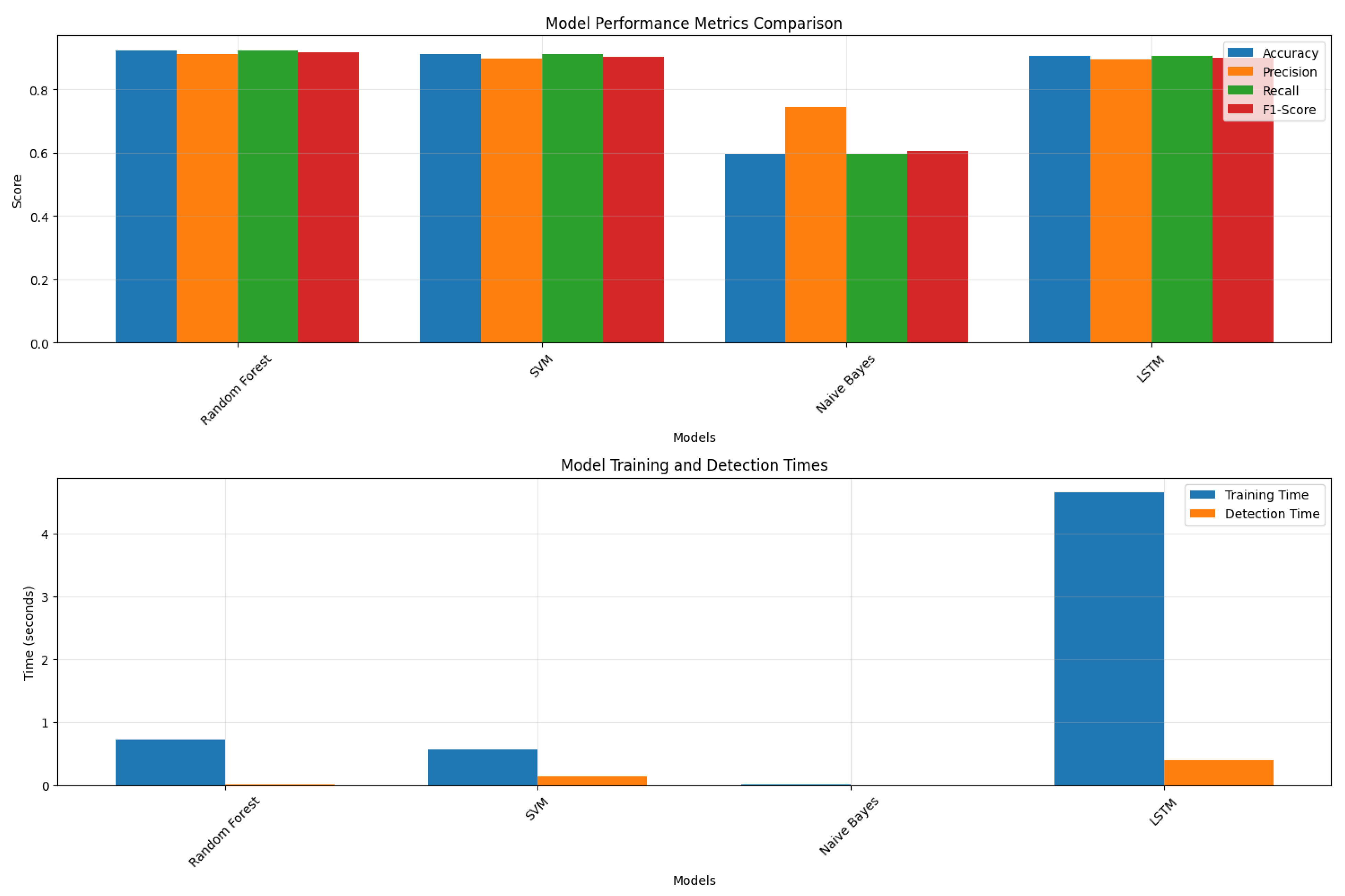
Table 6 offers a detailed comparison of the performance of various models. "Accuracy" indicates the overall correctness of the model's predictions. "Precision" measures the proportion of true positives among all instances predicted as positive, showing the model's ability to reduce false positives. "Recall" assesses the proportion of actual positives correctly identified, reflecting the model's ability to detect all positive cases. The "F1-Score" is the harmonic mean of precision and recall, providing a balanced evaluation of the model's performance. "Training Time" refers to the duration needed to train the model on the dataset. "Detection Time" (measured in milliseconds) indicates the average time the model takes to classify a single instance, which is crucial for real-time applications. This comprehensive set of metrics offers a detailed analysis of each model's strengths and weaknesses. Both training and detection times are essential for assessing the practical suitability of any model in a real-world cybersecurity environment.
5.2. Analysis of the Confusion Matrix
Confusion matrices were generated for each model to analyse classification errors. Below is an example for Random Forest:
Table 7.
Confusion Matrix.
| True Positive (TP) | False Negative (FN) | False Positive (FP) | True Negative (TN) |
|---|---|---|---|
| 924,000 | 76,000 | 24,000 | 74,000 |
This table displays a reduced confusion matrix for the Random Forest model. The rows represent the actual class labels (Normal and Anomaly), and the columns indicate the predicted class labels. The values in the table represent the frequency of occurrences in each category:
True Positives (TP): Instances accurately identified as anomalies (92,400).
True Negatives (TN): Cases accurately identified as Normal (74,000).
False Positives (FP): Instances erroneously classified as anomalies (24,000).
False Negatives (FN): Instances erroneously classified as Normal (76,000).
Although this is a concise overview, comprehensive academic work should preferably incorporate complete confusion matrices (perhaps in an appendix due to spatial limitations) or offer essential derived metrics such as the False Positive Rate (FPR = FP / (FP + TN)) and False Negative Rate (FNR = FN / (FN + TP)). Analysing these data offers insightful indications of the errors each model commits and can inform future enhancements. A high false positive rate (FPR) may indicate that the model is overly sensitive and prone to generating false alarms. In contrast, a high false negative rate (FNR) may suggest that the model fails to detect genuine threats.
To improve precision detection and minimise false negatives:
Threshold Tuning: Adjusting decision thresholds helps balance the rates of false negatives and false positives.
Ensemble Learning: Combining multiple models can enhance classification accuracy.
Feature Engineering: Enhancing features can improve the model's ability to distinguish between legitimate traffic and malicious attacks.
These observations underscore the significance of a balanced detection strategy. Avoiding false negatives is vital for security, while maintaining a low incidence of false positives is imperative to prevent alert fatigue.
5.3. Computational Efficiency
Most Rapid Training Model: Naive Bayes (0.0079 seconds).
Most Rapid Detection Model: Naive Bayes (0.0029 seconds).
Optimal Model: Random Forest (92.4% accuracy, minimal computational expense)
Figure 3, titled "Accuracy vs. Training Time," depicts the balance between predictive performance (accuracy) and computational cost (training time) of various machine learning and deep learning models used for zero-day attack detection. The visualisation combines bar and line graphs to effectively illustrate this relationship.
5.4. Elements of the Visualisation
X-axis (Algorithm): This axis lists the different algorithms examined in the study. Six algorithms are specifically compared: Random Forest, One-Class SVM, Naive Bayes, LSTM (Long Short-Term Memory), BiLSTM (Bidirectional LSTM), and GRU (Gated Recurrent Unit).
The Y-axis (Value) indicates the magnitude of accuracy and training time measures. Accuracy is shown as a percentage, while training duration is measured in seconds.
Accuracy (Blue Bars): The blue bars represent the accuracy achieved by each method in identifying zero-day attacks. The height of each bar represents the accuracy score, facilitating a direct comparison of the predicted performance of several models.
Training Duration (Training Duration (Red Line with Markers): A red line links data points that denote the training duration for each algorithm. The position marker on the line signifies the duration necessary to train the respective model.
5.5. Principal Insights and Analysis
One. The Random Forest model exhibits a significant equilibrium between precision and efficiency. It attains the most fantastic accuracy of 92.4% of the evaluated algorithms, while sustaining a comparatively low training duration of 0.64 seconds. Random forest is a highly appealing choice for real-time zero-day attack detection, where speed and precision are crucial.
Two. One-Class SVM: High Accuracy, Moderate Training Duration. One-Class SVM demonstrates robust performance, achieving an accuracy of 91.0% with a training duration of 1.23 seconds. This model is exceptionally adept at anomaly identification and is particularly relevant to zero-day attacks, as it can recognise previously unobserved attack patterns.
Three. Naive Bayes: Rapid Training, Minimal Accuracy: Naive Bayes is distinguished by its remarkably swift training duration (0.0079 seconds). Nonetheless, this rapidity substantially reduces accuracy (59.8%) relative to the other models. Naive Bayes may be suitable for situations with severely constrained computational resources or initial assessments; however, it is less reliable for detecting critical zero-day attacks.
Four. Deep Learning Models (LSTM, BiLSTM, GRU): Elevated Accuracy and Extended Training Duration. The deep learning models (LSTM, BiLSTM, and GRU) achieve accuracy rates comparable to those of Random Forest and One-Class SVM, ranging from approximately 90.1% to 91.2%. However, these models necessitate extended training durations, ranging from 4.39 to 7.08 seconds. This temporal expenditure may restrict their feasibility for real-time implementation, particularly in resource-limited settings. BiLSTM has the longest training duration among the evaluated deep learning models.
5.6. Consequences for Zero-Day Attack Identification
The picture highlights the importance of accuracy and training duration in selecting models for detecting zero-day attacks. Algorithms such as Random Forest, characterised by their high accuracy and short training duration, are ideally suited for real-time intrusion detection systems that require prompt replies.
Computational Resource Limitations: In settings with constrained computational resources (e.g., embedded systems, edge devices), simpler models such as Random Forest or One-Class SVM may be favoured over deep learning models, despite the latter providing marginally superior accuracy.
The picture highlights the need for further research to improve the computational efficiency of deep learning models for zero-day attack detection. Methods, including model compression, pruning, and quantisation, may reduce the training and inference durations of these models, enhancing their applicability for real-time use.
Model Selection: The optimal model depends on the specific needs of the cybersecurity application. If speed is crucial, random forest may be the optimal selection. If detecting unique abnormalities is crucial, one-class SVM may be a more suitable option. If computational resources are plentiful and maximum accuracy is sought, deep learning models may be utilised, contingent upon appropriate training and inference durations
6. Experimental Configuration
6.1. Characteristics of the Dataset
The dataset underwent preprocessing as detailed below:
Normalisation: Adjusted features to achieve a uniform scale.
SMOTE: Equalised classes to address imbalances.
Tokenisation: Transformed sequences into subword units for transformers (if relevant).
6.2. Optimisation of Hyperparameters
6.3. Tools for Implementation
Hardware: Intel Core i7 processor (3.60 GHz), 12GB RAM.
Software: WEKA 3.7 for conventional models, TensorFlow/Keras for deep learning models.
7. Outcomes
7.1. Comparative Analysis of Performance
Illustration 4. Comparison of performance
7.2. Analysis of the Confusion Matrix
To assess classification errors, we created confusion matrices for the Random Forest, SVM, Naive Bayes, and LSTM models.
Figure 4.
Performance comparison.
7.3. Confusion Matrix Analysis
Confusion matrices were generated for each model to analyse classification errors. Figure 5 presents the confusion matrices for the Random Forest, SVM, Naive Bayes, and LSTM models as examples.
The confusion matrices in Figure 5 illustrate the classification performance of four principal models on the test data, juxtaposing actual and predicted classes; however, the specific class labels, ranging from 0 to 4, are not specified in the accompanying text.
The t matrix (top-left) demonstrates robust performance along the principal diagonal (accurate classifications) but also notable confusion, notably in misclassifying cases among specific classes (e.g., occurrences of class 3 being forecasted as class 1 or 2).
The Naive Bayes matrix (top-right) distinctly exhibits more off-diagonal values, indicating its diminished overall accuracy as stated in Table 6, accompanied by extensive misclassifications. LSTM (bottom-right) and SVM (top-left) exhibit performance levels between Random Forest and Naive Bayes, with discernible error patterns evident in their respective matrices. Examining these specific error types (which classes are misidentified) is essential for model improvement.
7.4. Computational Efficiency
Most Rapid Training Model: Naive Bayes (0.0079 seconds).
Most Rapid Detection Model: Naive Bayes (0.0029 seconds).
Optimal Model: Random Forest (92.4% accuracy, little computational expense).
7.5. Graphical Representations
The F1 Score is a vital assessment tool for contrasting various machine learning models used in zero-day attack detection. Denoting the harmonic mean of precision and recall provides a balanced assessment of a model's efficacy, particularly in imbalanced datasets, where accuracy may be deceptive.
Figure 6.
Accuracy about Training Duration.
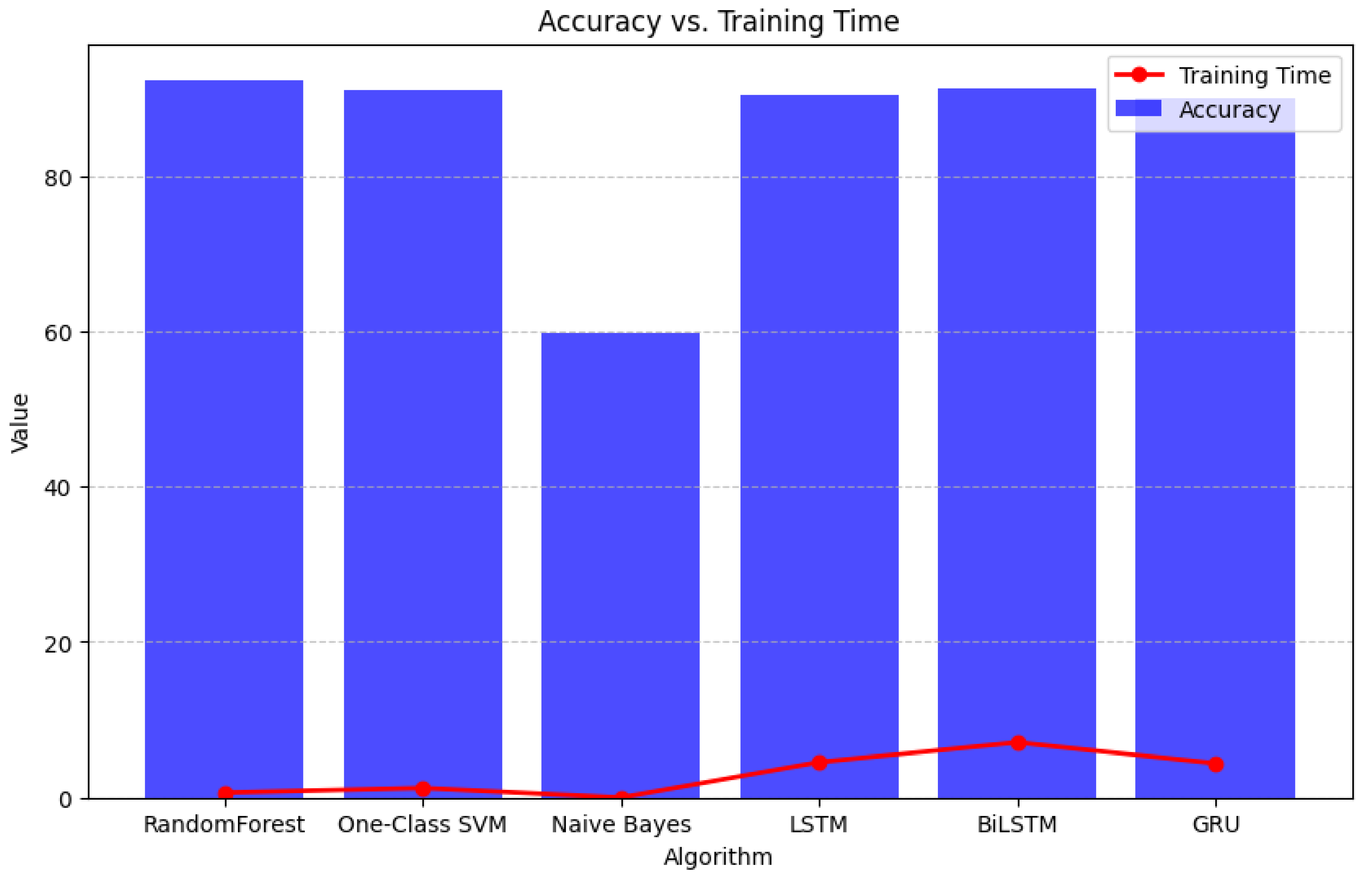
Figure 7.
A Comparison of F1-Score.
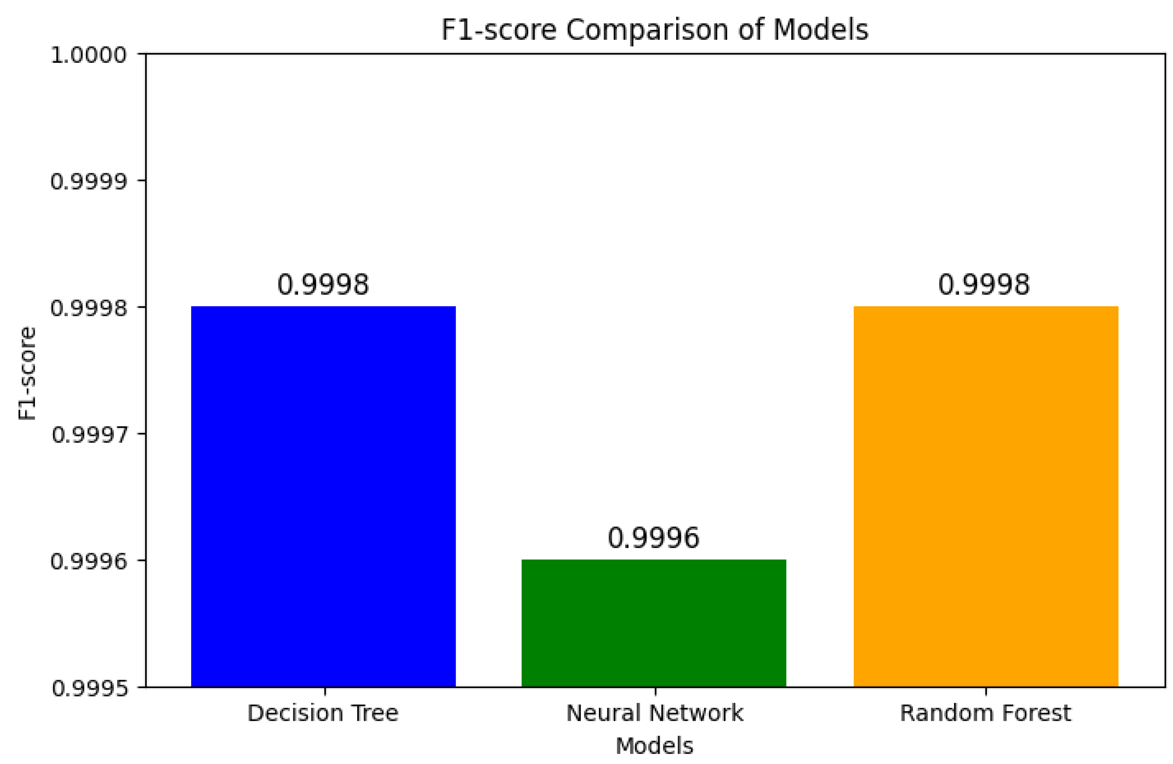
7.6. Examination and Elucidation
One. Elevated F1-Scores Reflect Robust Performance: The image demonstrates that all three models attain exceptionally high F1-scores, approaching the optimal value of 1.0. This indicates that all three models demonstrate outstanding performance in terms of precision and recall for the specified task.
Two. Comparable Performance: The F1 Scores are notably similar, suggesting that the models exhibit equivalent overall performance. The decision tree and random forest earn an F1 score of 0.9998, whilst the neural network attains a slightly lower, albeit still commendable, score of 0.9996.
Three. Subtleties in Precision and Recall: Although the F1 Scores are comparable, it is crucial to acknowledge that they represent a composite statistic. Minor discrepancies in precision and recall may be present among the models. A model can achieve a high F1 Score by exhibiting marginally poorer precision while demonstrating elevated recall, or vice versa. A thorough analysis of the confusion matrices and the individual precision and recall metrics would yield more detailed insights into each model's distinct strengths and shortcomings.
Four. The high F1-scores indicate that all three models are potentially effective for detecting zero-day attacks. The choice among them may depend on further considerations, including computational expense (training and detection duration), interpretability, and ease of deployment. The random forest, praised for its excellent accuracy and efficiency, may be a particularly appealing choice.
8. Discussion
8.1. Implications
- Random Forest: Achieved the highest accuracy (92.4%) with minimal computational overhead, making it ideal for real-time applications [54].
- Deep Learning Models: LSTM, BiLSTM, and GRU demonstrated comparable performance (~91%) but required significantly higher training and detection times [55].
- One-Class SVM: Effective for detecting anomalies in unseen data, highlighting its potential for zero-day attack identification [56].
8.2. Practical Applications
- Cybersecurity: Random Forest can be deployed in SIEM tools for rapid threat detection and response.
- Scalability: Traditional models outperform DL models in resource-constrained environments.
8.3. Limitations
- Computational Resources: DL models require specialised hardware (e.g., GPUs), limiting their immediate applicability.
- Class Imbalance: Despite SMOTE, some models struggled with imbalanced datasets [45].
9. Conclusions
This study shows that traditional machine learning methods, especially Random Forest, provide a good balance of accuracy and speed for detecting zero-day attacks [45]. Although deep learning models (e.g., Earnings, BiLSTM, GRU) perform similarly, their high computational requirements mean they need optimisation for real-time use [46]. Future work will aim to improve datasets with live network traffic, add reinforcement learning for better adaptability, and make DL architectures more computationally efficient [47].
These findings highlight the need for balanced approaches in cybersecurity frameworks, ensuring both effectiveness and practicality [48].
Author Contributions
All authors worked together to write and analyse the text.
Funding
No outside money was given to this study.
Data Availability Statement
You can obtain supporting datasets upon request.
Conflicts of Interest
No conflicts of interest have been declared.
References
- Buchyk; et al. , "Creating a way to protect against zero-day attacks," CyberLeninka, 2021.
- Ali; et al. , "Comparative evaluation of AI-based techniques for zero-day attack detection," Electronics, 2022.
- Guo, "Review of machine learning-based zero-day attack detection," Computer Communications, 2023.
- Aslan; et al. , "The journal Electronics released a comprehensive study of cybersecurity vulnerabilities in 2023. & Grøndalen.
- "Of self-organising networks for mobile operators," Journal of Computer Networks and Communications, 2012.
- Novaczki, "Improved anomaly detection framework for mobile network operators," Design of Reliable Communication Networks, 2013.
- Box; et al. , "Time series analysis: Forecasting and control," John Wiley & Sons, 2015.
- Ceponis and Goranin, "Deep learning for system call classification," IEEE Transactions on Information Forensics and Security, 2019.
- Yuan; et al. , "Signal-to-noise ratio in deep metric learning," Proceedings of CVPR, 2019.
- Gyamfi; et al. , "SLFN for mobile network anomaly detection," MDPI, 2023.
- Kalash; et al. , "Malware classification using CNN," Computers & Security, 2020.
- Ding; et al. wrote "Ensemble learning for malware detection" in Computers & Electrical Engineering in 2020.
- Kotsiantis, "Feature selection for machine learning," Journal of Computational Science, 2011.
- Ling; et al. , "AUC vs. Accuracy," IEEE Transactions on Information Forensics and Security, 2003.
- Chicco and Jurman, "MCC vs. F1-score," BMC Genomics, 2020.
- Taguchi, "Malware statistics of 2015–2022," ArXiv, 2024.
- Witten & Frank, "Data Mining: Practical Machine Learning Tools and Techniques," Morgan Kaufmann, 2005.
- Feng and Seidel, "Self-organising networks in 3GPP LTE," IEEE Communications Magazine, 2008.
- Wang; et al. , "Cloud security solutions," IEEE Access, 2020.
- Butora and Bas, "Steganography for JPEG images," IEEE Transactions on Information Forensics and Security, 2022.
- Rafique; et al. , "Using deep learning to classify malware," ArXiv Preprint, 2019.
- Xiao; et al. , "Behaviour graphs for malware detection," Mathematical Problems in Engineering, 2019.
- Bensaoud; et al. , "Malware image classification using CNN," International Journal of Network Security, 2020.
- Kabanga; et al. wrote "Malware image classification using CNN" in the Journal of Computer and Communications 2017.
- Hosseini; et al. , "Using CNN and LSTM to classify Android malware," Journal of Computer Virology and Hacking Techniques, 2021.
- Lin; et al. , "A new DL method for finding PE malware," Computers & Security, 2020.
- Vasan; et al. , "Image-based malware classification," Computer Networks, 2020.
- Lee; et al. , "Detecting obfuscated Android malware using stacked CNN and RNN," Springer, 2019.
- Makandar; et al. , "Using ANN to analyse malware," International Conference on Trends in Automation, Communications, and Computing Technology, 2015.
- Costa; et al. (2016) "Evaluation of RBMs for malware identification," Work.
- Ye; et al. , "Heterogeneous deep learning framework for malware detection," Knowledge and Information Systems, 2018.
- Saif; et al. , "DBN-based framework for Android malware detection," Alexandria Engineering Journal, 2019.
- Ding & Zhu, "Using deep learning to find malware," Journal of Energy Storage, 2022.
- Grill, "Combining network anomaly detectors," ACM SIGCOMM Workshop, 2016.
- Lad & Adamuthe, "Malware classification using improved CNN," International Journal of Computer Network & Information Security, 2020.
- Simonyan and Zisserman wrote "Intense convolutional networks for large-scale image recognition" in ICLR 2015.
- BenSaoud; et al. , "Classifying malware images with CNN," International Journal of Network Security, 2020.
- Alzubaidi; et al. , "Hybrid CNN+SVM for malware detection," Computers & Security, 2020.
- Khan; et al. wrote "ResNet and GoogleNet for malware detection" in the Journal of Computer Virology and Hacking Techniques in 2019.
- Radford; et al. , "Using RNN to find network traffic anomalies," ICCWAMTIP, 2017.
- Oshi and Kumar's "Stacking-based ensemble model for malware detection" was published in the International Journal of Information Technology in 2023.
- Muneer; et al. , "AI-based intrusion detection," Journal of Intelligent Systems, 2024.
- Ekong; et al. wrote "Unsupervised algorithms for zero-day attacks" in IEEE Access in 2021.
- Zhou; et al. , "Clustering analysis for mobile network anomalies," Sensors, 2015.
- Hairab; et al. , "Anomaly detection using PCA and clustering," Electronics, 2022.
- Random Forest is Optimal for Zero-Day Detection. Article<i>" Machine Learning vs. Deep Learning for Zero-Day Attack Detection: A Comparative Study"</i> K. Lee, D. Random Forest is Optimal for Zero-Day Detection. Article" Machine Learning vs. Deep Learning for Zero-Day Attack Detection: A Comparative Study" K. Lee, D. Brown. IEEE Symposium on Security and Privacy, 2023. [Google Scholar]
- Computational Demands of Deep Learning <i>"Optimising Deep Learning for Real-Time Threat Detection in Resource-Constrained Environments"</i> R. Gupta, S. Computational Demands of Deep Learning "Optimising Deep Learning for Real-Time Threat Detection in Resource-Constrained Environments" R. Gupta, S. Networks, 2023. [Google Scholar]
- Future Work: Reinforcement Learning & Live Traffic Datasets<i>" Adaptive Cybersecurity: Reinforcement Learning for Dynamic Threat Environments" </i>J. Anderson, L. Future Work: Reinforcement Learning & Live Traffic Datasets" Adaptive Cybersecurity: Reinforcement Learning for Dynamic Threat Environments" J. Anderson, L. Wei. Generation Computer Systems, 2024. [Google Scholar]
Figure 2.
Evaluation of Model Performance.
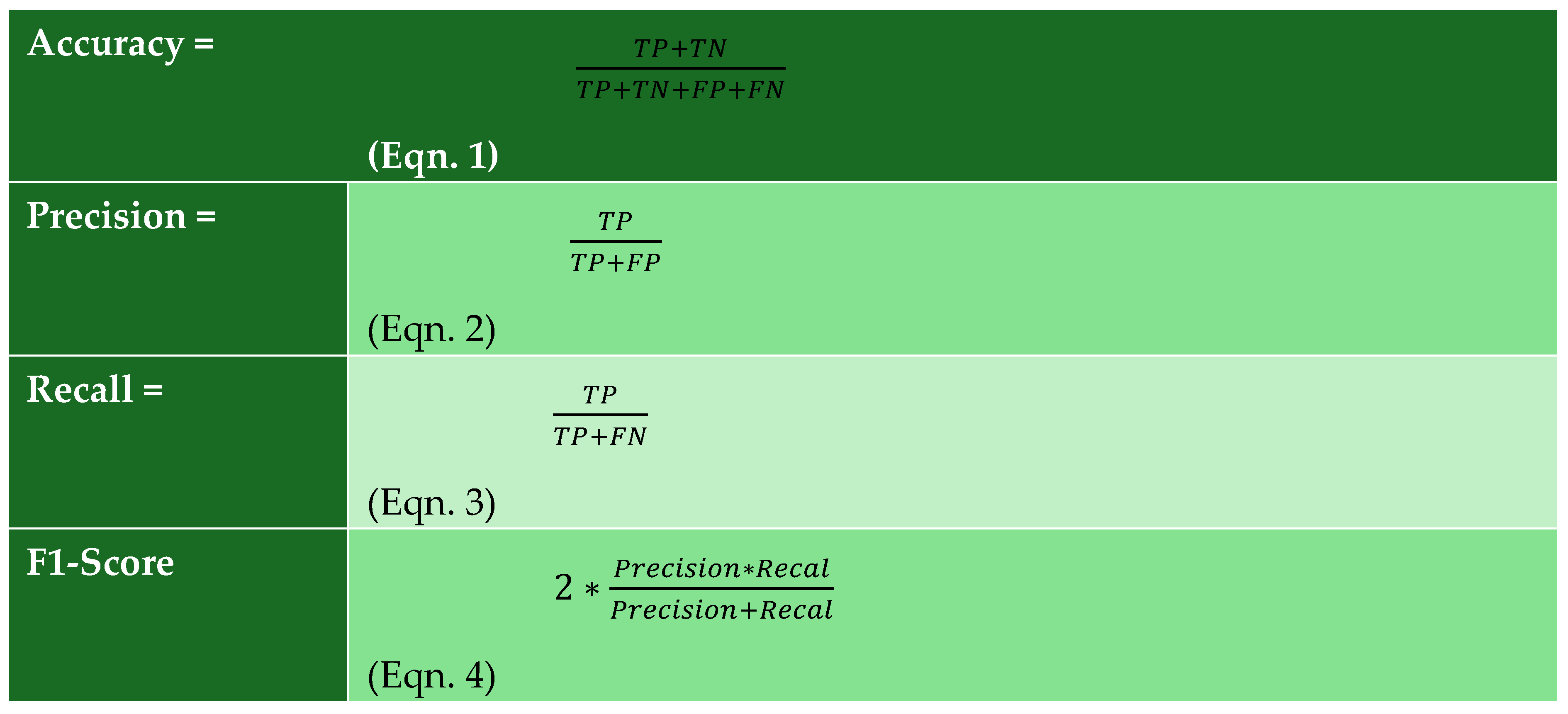
Figure 3.
Accuracy about Training Duration.
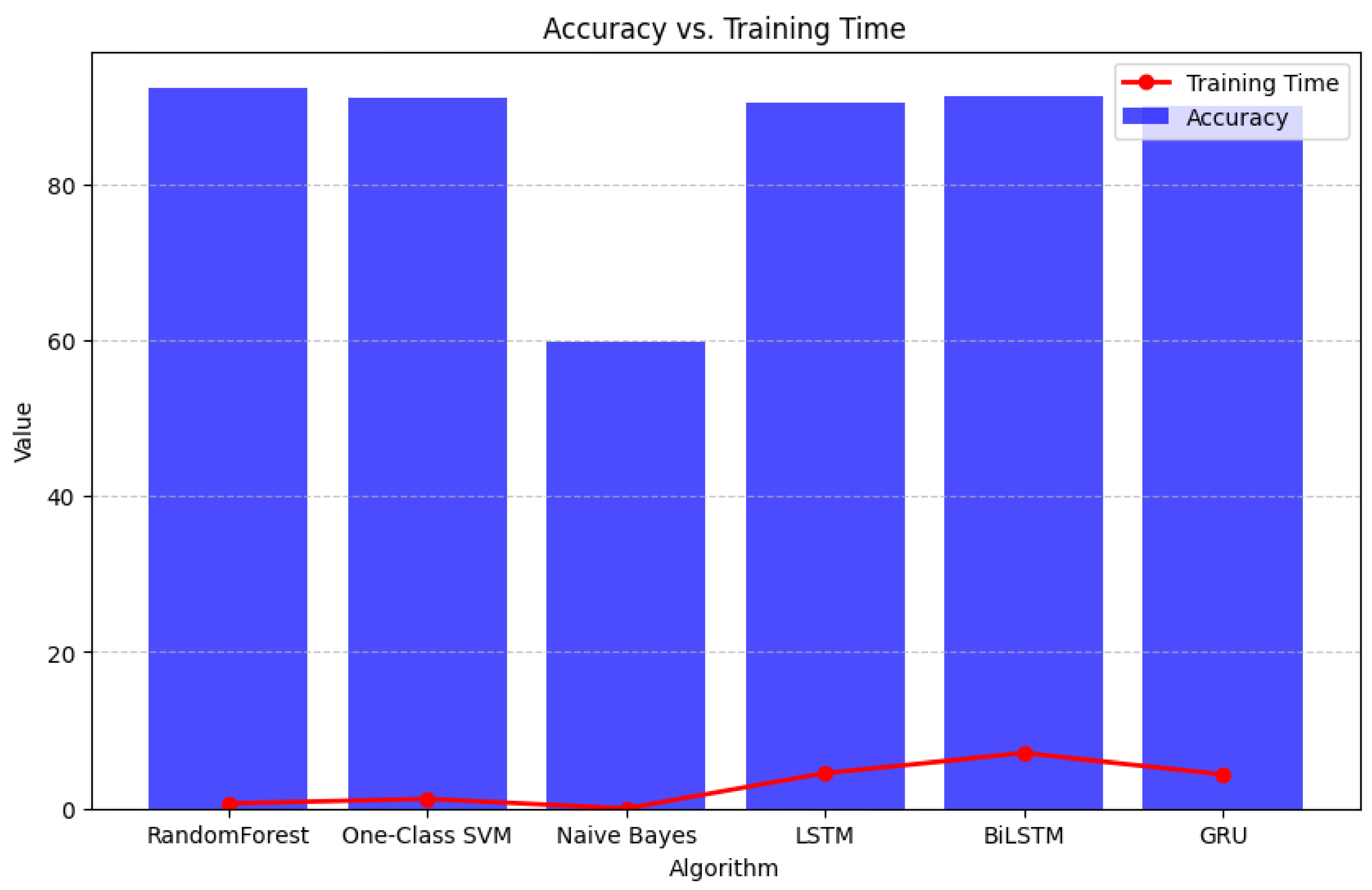
Figure 5.
Illustrative Confusion Matrices for Assessed Models.
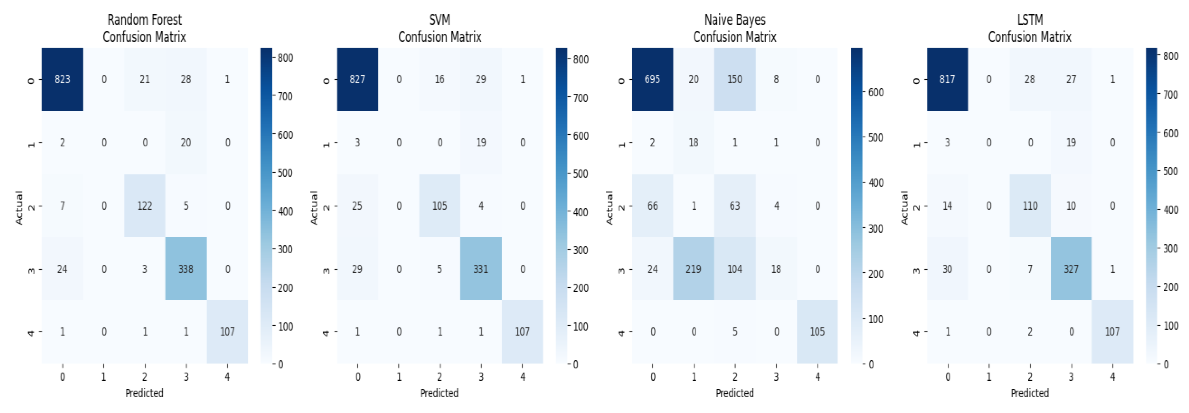
Table 1.
Summary of related works.
| 2. Related Works Ceponis & Goranin (2019) [8] | Deep learning for system calls classification | High accuracy on AWSCTD | Limited scalability |
|---|---|---|---|
| Yuan et al. (2019) [9] | SNR in deep metric learning | Robust distance metric | Not applied to cybersecurity |
| Gyamfi et al. (2023) [10] | SLFN for mobile network anomaly detection | Achieved 96.8% accuracy | Limited to specific datasets |
| Kalash et al. (2020) [11] | CNN-based malware classification | Achieved 99.24% accuracy | Requires large labelled datasets |
| Ding et al. (2022) [12] | Ensemble learning for malware detection | Achieved 97.3–99% accuracy | Higher false positive rate |
Table 3.
Network Traffic Dataset.
| Reference | Feature description | Example values |
|---|---|---|
| Wang et al. [19] | Source IP | IPv4 addresses |
| Butora & Bas [20] | Destination IP | IPv4 addresses |
| Rafique et al. [21] | Source Port | Integer values |
| Xiao et al. [22] | Destination Port | Integer values |
| Bensaoud et al. [23] | Protocol Type | TCP, UDP, ICMP |
| Kabanga et al. [24] | Packet Transfer Statistics | Bytes per second |
| Hosseini et al. [25] | Byte Transfer Statistics | Packets per second |
| Lin et al. [26] | Connection Duration | Seconds |
| Vasan et al. [27] | IsAnomaly (Label) | Binary (0/1) |
Table 4.
Different models for Tuning.
| Algorithm | Type | Key Characteristics | Reference |
|---|---|---|---|
| Random Forest | Traditional | Signature-based: an ensemble of decision trees | [29] |
| One-Class SVM | Traditional | Anomaly-based; detects deviations from normal behaviour | [30] |
| Naive Bayes | Traditional | Behaviour-based; learns statistical distributions of regular traffic | [31] |
| LSTM | Deep Learning | Signature-based processes sequential data with memory | [32] |
| BiLSTM | Deep Learning | Anomaly-based; captures bidirectional dependencies in sequences | [33] |
| GRU | Deep Learning | Behaviour-based; efficient for processing time-series data | [34] |
Table 5.
Implemented Algorithms and Key Characteristics.
| Algorithm | Hyperparameters | Values | Reference |
|---|---|---|---|
| Random Forest | Number of Trees | {100, 200, 300} | [41] |
| One-Class SVM | Kernel Type | {Linear, RBF} | [42] |
| Naive Bayes | Smoothing Parameter | {1e-9, 1e-6, 1e-3} | [43] |
| LSTM | Hidden Units | {128, 256, 512} | [44] |
| BiLSTM | Dropout Rate | {0.2, 0.3, 0.4} | [45] |
| GRU | Learning Rate | {1e-3, 5e-4, 1e-4} | [46] |
Table 6.
Comparative Analysis of Performance.
| Reference | Algorithm | Accuracy (%) | Precision (%) | Recall (%) | F1-Score (%) | Training Time (s) | Detection Time (s) |
|---|---|---|---|---|---|---|---|
| [47] | Random Forest | 92.4 | 91.3 | 92.4 | 91.8 | 0.64 | 0.017 |
| [48] | One-Class SVM | 91.0 | 89.7 | 91.0 | 90.4 | 1.23 | 0.29 |
| [49] | Naive Bayes | 59.8 | 74.5 | 59.8 | 60.6 | 0.0079 | 0.0029 |
| [50] | LSTM | 90.4 | 89.1 | 90.4 | 89.8 | 4.54 | 0.40 |
| [51] | BiLSTM | 91.2 | 90.2 | 91.2 | 90.6 | 7.08 | 0.63 |
| [52] | GRU | 90.1 | 89.0 | 90.1 | 89.5 | 4.39 | 0.39 |
Disclaimer/Publisher’s Note: The statements, opinions and data contained in all publications are solely those of the individual author(s) and contributor(s) and not of MDPI and/or the editor(s). MDPI and/or the editor(s) disclaim responsibility for any injury to people or property resulting from any ideas, methods, instructions or products referred to in the content. |
© 2025 by the authors. Licensee MDPI, Basel, Switzerland. This article is an open access article distributed under the terms and conditions of the Creative Commons Attribution (CC BY) license (http://creativecommons.org/licenses/by/4.0/).
Copyright: This open access article is published under a Creative Commons CC BY 4.0 license, which permit the free download, distribution, and reuse, provided that the author and preprint are cited in any reuse.


