
Submitted:
30 June 2025
Posted:
02 July 2025
You are already at the latest version
Abstract
This study explores the behavior of phantom dark energy within the framework of Weyl-type
$f(Q,T)$ gravity, considering a spatially flat FLRW universe under observational constraints. The field equations are analytically solved for a dust-like fluid source. To determine the present values of the model parameters, we utilize observational data from the Hubble parameter measurements via cosmic chronometers (CC) and the apparent magnitude data from the Pantheon compilation of Type Ia supernovae (SNe Ia).With these obtained parameter values, we analyze the model’s physical characteristics by evaluating the effective and dark energy equation of state parameters $\omega_{eff}$ and $\omega_{de}$
, the deceleration parameter $q(z)$, and energy conditions. Additionally, we conduct the $O_{m}$ diagnostic test for the model. We estimate the transition redshift $z_{t}\le0.5342, 0.6334$ and the present age of the universe $t_{0}=13.46, 13.49$ Gyrs with $H_{0}=67.4\pm3.6, 68.8\pm1.9$ Km/s/Mpc, $\Omega_{m0}=0.41_{-0.24}^{+0.13}, 0.299_{-0.077}^{+0.042}$, and $\omega_{eff}=-0.6447, -0.696$, $\omega_{de}=-1.0347, -1.0284$. We find a transit phase accelerating and physically acceptable phantom dark energy model of the universe.
Keywords:
FLRW universe
; Weyl-type $f(Q
; T)$ gravity
; dark energy
; observational constraints
; om diagnostic
1. Introduction
Recent observational studies in [1,2,3,4,5,6,7] confirmed that the universe entered into an accelerating expansion phase six giga-years ago. This behavior of the universe suggests that it has some unknown components having high negative pressure and in a huge amount, approximately , which are so-called dark energy (DE) and dark matter (DM). To understand the unknown parts of the universe, researchers have suggested different theories of gravity over the past few decades. These theories add to general relativity (GR), which is the most successful theory used to study the universe. Some updated theories of gravity, like gravity (first introduced in [8]) and its extension called gravity [9], are based on linking the trace T of the energy-momentum tensor to . There are many other similar theories in Riemannian geometry.
Alternatively, in non-Riemannian geometry, the teleparallel gravity () [10,11,12,13] and the symmetric teleparallel gravity () [14,15] are developed in the same way as the Riemannian gravity theory (). Here, the torsion scalar T and the non-metricity scalar Q, respectively, replace R. A new paper [16] describes the gravity theory, which adds to the gravity theory by connecting it to the trace T of the energy momentum tensor in a way that is not minimal. They examined the cosmological implications of three distinct models inside the theory. Their results, together with the solution, delineated both the speeding and decelerating evolutionary phases of the universe. Several studies have shown that gravity is a reasonable way to explain how fast the universe is expanding right now and provide a logical answer to the dark energy puzzle [17,18,19].
Weyl gravity extends General Relativity (GR) by incorporating non-metricity within the affine connection, aiming to unify gravity and electromagnetism. Recent studies, such as [20], have explored its implications for dark matter and dark energy. In particular, [21] investigates a non-minimal coupling between the trace T and the non-metricity scalar Q within the framework of Weyl gravity. This concept was further refined by [22], introducing Weyl-type gravity, where non-metricity is entirely determined by the magnitude of the vector field . In Weyl geometry, gravitational field equations emerge by varying the action with respect to the metric tensor, with the vector field playing a crucial role in describing gravitational interactions. Despite being a relatively new approach, Weyl-type gravity has been extensively applied in various cosmological contexts. Works such as [23,24,25] examine its impact on cosmic acceleration, the Newtonian limit, geodesic and Raychaudhuri equations, tidal forces, and power-law solutions, shedding light on the broader implications of this modified gravity theory.
Recently, [26] created a space model in a type of gravity called Weyl-type by using a specific way to express the Hubble parameter. Meanwhile, [27] looked into a model with friction in this same gravity theory. A cosmological model has been created using a method that does not rely on specific assumptions, along with observational evidence, as mentioned in references [28,29]. Additionally, an interaction related to a deceleration parameter that does not change over time is explored in [30], focusing on a type of gravity called Weyl-type . We use model-independent techniques to construct most of the previously discussed models in Weyl-type gravity. In the present paper, we develop a cosmological model based on the exact solutions to the cosmological field equations. We build a CDM model with a perfect fluid source in the Weyl-type gravity theory. We use Hubble data from cosmic chronometer (CC) observations and apparent magnitude from the Pantheon sample of SNe Ia to put limits on our model.
The paper is organized into the following sections. Sect.-1 contains a brief introduction to the development of cosmological models. Sect.-2 provides a brief overview of Weyl-type gravity, while Sect.-3 mentions the cosmological field equations. We obtain an analytical solution to the field equations in Sect. 4; Sect. 5 contains some observational constraints on solutions. We discuss the results in Sect.-6, and finally, we present our conclusions in Sect.-7.
2. Brief Concept of Weyl Type Gravity
We consider the following action to derive the field equations in the Weyl-type -gravity [22]:
where is an intrinsic vector field with a semi-metric connection , introduced by Weyl to generalize the Riemannian geometry in order to describe the simultaneous change of direction and length. The semi-metric connection is given by
where is the Christoffel symbol constructed with respect to the metric . The is the Weyl length curvature tensor defined by
and , where R denotes the Ricci scalar curvature associated with the Levi-Civita connection. , , The mass of the particle is denoted as m, while represents the ordinary matter Lagrangian. Moreover, f denotes a general function of the non-metricity scalar. Q and T correspond to the trace of the energy-momentum tensor linked to matter. The second and third terms in the action describe the standard kinetic term and the mass term related to the vector field, respectively. The non-metricity scalar Q is given by
where, the deformation tensor is defined as
In Riemannian geometry i.e., the Levi-Civita connection is metric compatible while in the case of semi-metric connection in weyl geometry, we have
which are not vanishing at all.
By differentiating the variation of action (1) with respect to the vector field , we derive the generalized Proca equation that describes the evolution of the field.
Through a comparison of Eq. (8) with the standard Proca equation, we can derive the effective dynamical mass of the vector field as
Once more, the variation of the action (1) concerning the metric field yields the subsequent modified field equations:
where, the energy-momentum tensor for matter is given by
and
The terms represent the partial derivatives of the arbitrary function with respect to T and Q, respectively. Additionally, the expression is defined as follows.
Here, is the re-scaled energy momentum tensor of the free Proca field,
3. Cosmological Field Equations
For the investigation of an isotropic, homogeneous and spatially flat universe in the context of Weyl type theory, we consider Friedmann-Robertson-Walker metric given by
where is the scale factor depending upon t only. In a spatially symmetric spacetime, taking the vector field of the form
Hence, , which implies that
Now, we define the stress-energy-momentum tensor corresponding to metric (15) as
where is the four-velocity vector in a comoving coordinate system with and as the Hubble parameter. Also, we consider the corresponding Lagrangian of the perfect fluid source .
The constraints of flat space and the generalized Proca equation in the context of cosmology can be expressed as
By eliminating all the derivatives of using Eqs. (20) and (21), we obtain the set of cosmological field equations (22) and (23) in the form
The equation of continuity for the model is obtained as
By considering the limiting case where , , and , the gravitational action given in Eq. (1) simplifies to the conventional Hilbert-Einstein form. Under these conditions, the dark energy density and pressure vanish (, ), leading Eqs. (27) and (28) to reduce to the standard Friedmann equations in general relativity: and .
4. Cosmological Solutions
We investigate the linear form of the Lagrangian function suggested in [22], given by
Hence, we have
We solve the field equations for a dusty universe () with and using Eqs. (31) and (32) in (26), we get
Integrating equation (33), we get the matter energy density as
Now, for simplicity, we take a solution of Eq. (20) as , and using in Eq. (25), we have
Using Eq. (34) with the relation , [31] in Eq. (35), we have
where and . Integrating (36), we get
where , and hence, at present
The effective equation of state parameter is defined as
5. Cosmological Constraints
The expansion rate of the universe can be easily understood by the analysis of Hubble data points from cosmic chronometer (CC) observations [32,33] and apparent magnitudes from the Pantheon sample of SNe Ia observations [34]. To analyze different cosmological measures and study the expansion phase, we use the emcee software to conduct MCMC analysis on CC and Pantheon datasets. This involves minimizing the function and maximizing the likelihood function, which is related to by the formula , while applying appropriate prior information.
5.1. Hubble Data
In this section, we use 31 data points of H(z) from redshift values between 0.07 and 1.965. These measurements were taken using the differential age method and do not affect one another. Hence, we use the following formula:
where are the cosmological parameters which we have to estimated, and , are the observational and theoretical values of at , respectively. The denotes the standard deviations associated with observed values .
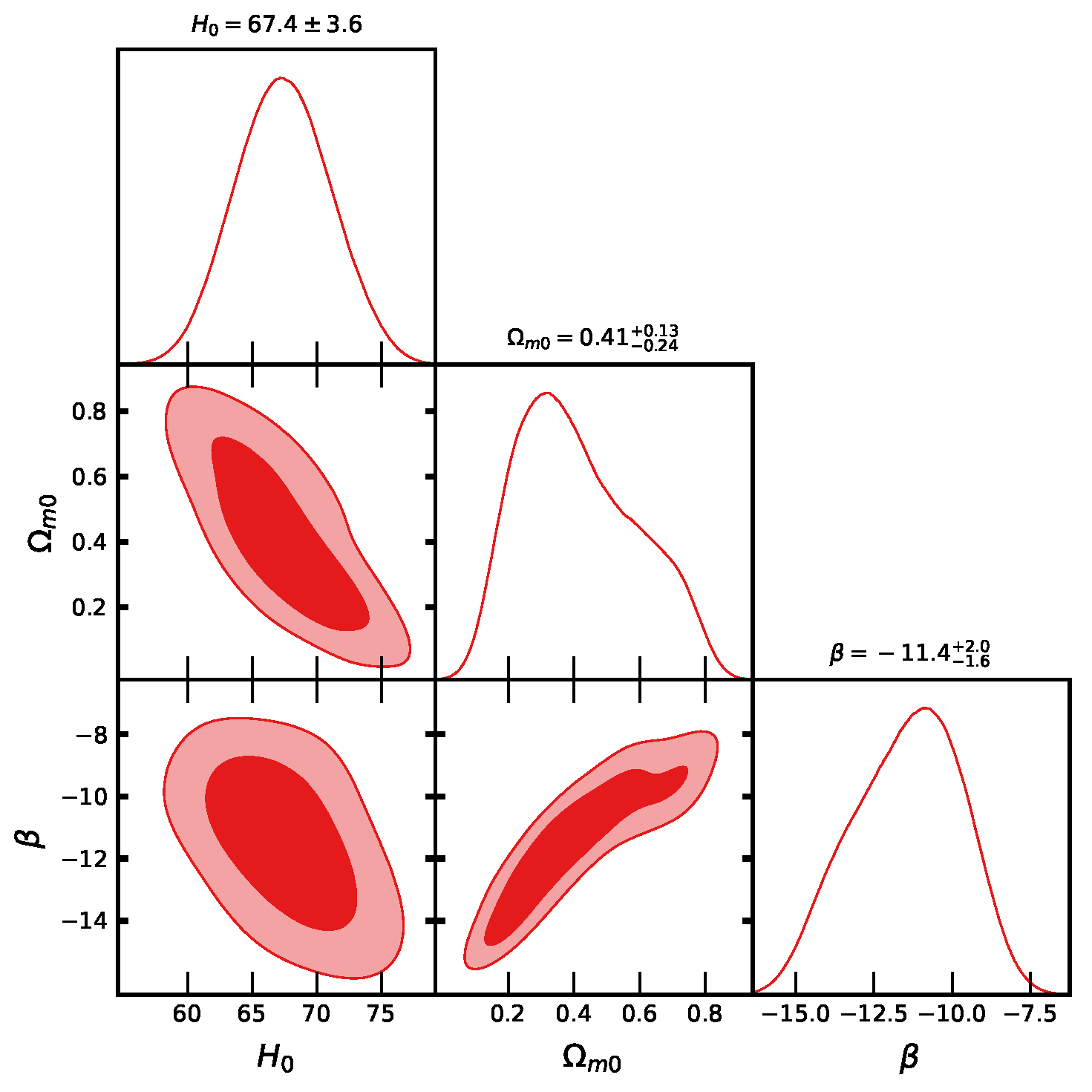
Figure 1.
The contour plots of at , confidence levels for CC dataset.
5.2. Apparent Magnitude
SNe Ia data is used to illustrate the measurement of the expansion rate of the cosmic evolution of the universe in the form of apparent magnitude . We analyzed the theoretical notion of apparent magnitude, as outlined in [34,35,36,37].
Here, M represents the absolute magnitude, while the luminosity distance is expressed in length units and defined as follows.
The Hubble-independent luminosity distance is expressed as , making it a dimensionless parameter. Consequently, the apparent magnitude is given by:
We identified a correlation between and M in the previously discussed equation, which remains unchanged within the CDM framework [34,37]. To address this degeneracy, we redefine these parameters as follows:
In this context, the parameter is a dimensionless quantity defined by the relation , where the Hubble constant is expressed as km/s/Mpc. It is noteworthy that, in most studies [38,39], this degenerate combination is often marginalized. However, recent investigations [40,41,42,43,44] suggest that such an approach might result in the omission of crucial physical insights. Specifically, a cosmological model featuring an abrupt transition in the absolute magnitude M at a low redshift has the potential to simultaneously address both the and growth tensions [45,46,47,48,49,50]. Consequently, we opt to retain this degenerate parameter in our estimation procedure.
Within the CDM framework, has been calibrated to a value of , as reported in [34]. The parameter exhibits variation across different cosmological models (see [34,40,41,42,43,44,45,46,47,48,49,50]). For analyzing the Pantheon dataset, we employ the following formulation, as outlined in [34].
The formula shows the difference between the observed value and the expected value found in equation (47). The notation represents the inverse of the covariance matrix derived from the Pantheon sample.
To estimate the model parameters jointly, we use 31 cosmic chronometer (CC) data points for the Hubble parameter along with 1,048 data points from the Pantheon dataset. By applying the formula, we perform a combined Markov Chain Monte Carlo (MCMC) analysis, integrating both Pantheon and CC data. This approach allows us to derive unified constraints on the parameters across all considered models.
Figure 2.
The contour plots of and at , confidence levels for CC+Pantheon datasets.
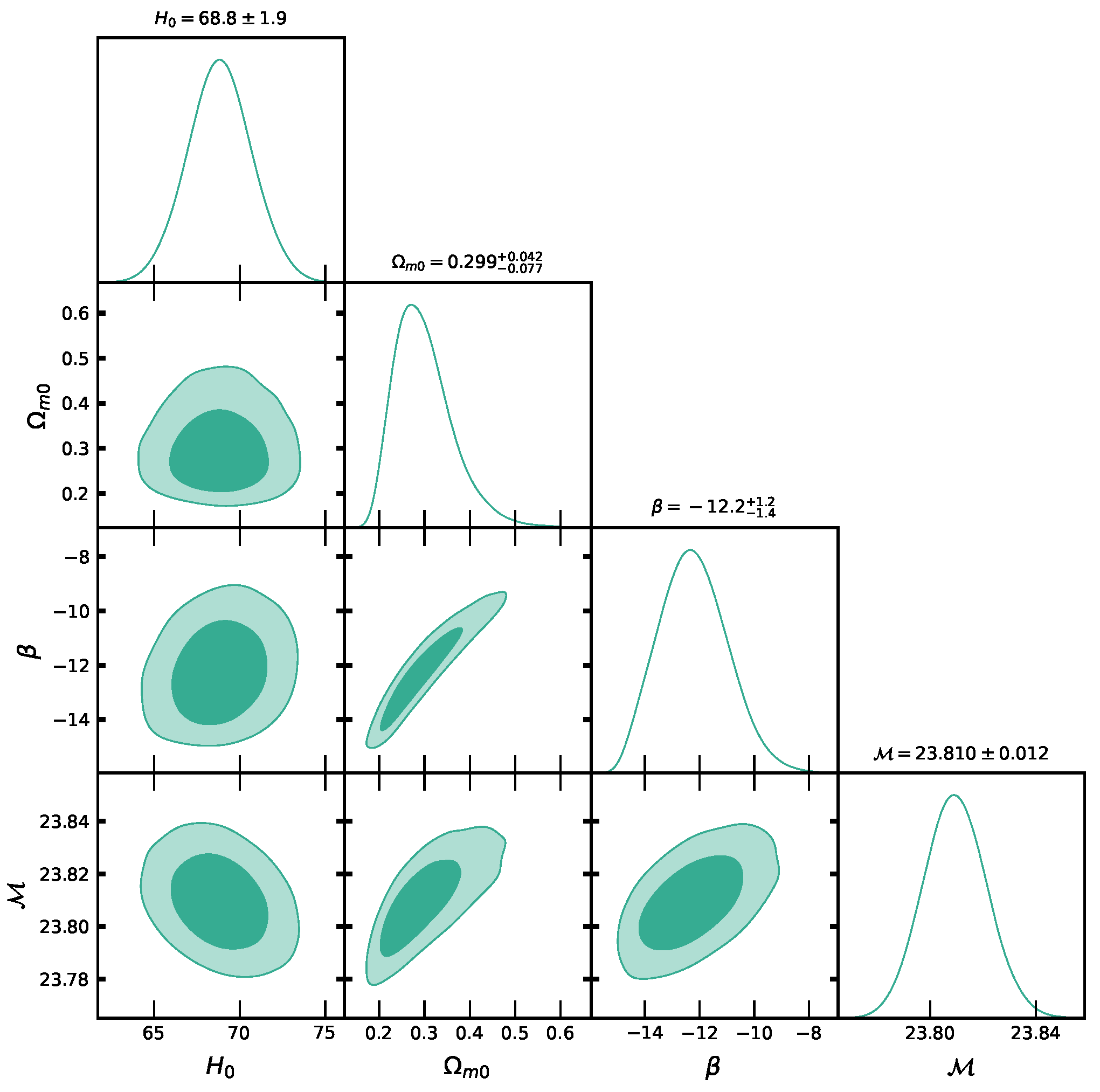
The Hubble function (37) contains six parameters, and to estimate them independently, we remove the degeneracy between them. For this, we choose , , and , as suggested in [22], and thus the Hubble function is reduced in terms of three independent parameters: , and . Table 1 shows the estimated values of these parameters using the CC and CC+Pantheon datasets with MCMC analysis.
6. Result Discussions
In this section, we discuss the output of our derived universe model in Weyl-type gravity. We found a precise solution to the updated field equations that involve a dust-like fluid. We also created a relationship between the model’s parameters and the Hubble function . Next, we estimate the values of the model parameters , , and by analyzing data from 31 CC datasets and 1048 Pantheon datasets using a method called MCMC. We do this at two confidence levels, and . We get the estimated values of the Hubble constant Km/s/Mpc, along with CC data, and Km/s/Mpc along with joint data CC+Pantheon. We get the values of baryonic matter density parameter , and dimensionless model parameter , along two observational datasets, respectively. The estimated values of the Hubble constant and matter density parameter are in good agreement with recent estimated values in [51,52,53,54,55,56,57,58]. We have non-vanishing dimensionless parameters , , , and m in the relation with . If we take , and , then vector field mass .
The change in the effective equation of state parameter, , shows the matter phase. Its formula is found in Eq. (43). The geometrical behavior of over z is shown in Figure 3a. From Figure 3a, one can observe that is an increasing function of z, and it tends to the CDM value when . We have calculated the current values of the effective equation of state parameters, which are and , based on observational data. These values are in excellent agreement with recent observations. Figure 3b depicts the evolution of the dark energy EoS parameter versus z. In Figure 3b, you can see that the value of crosses -1 (which is the value for the CDM model) and approaches this value again in the far future. We estimated the current value of the dark energy EoS parameter as along CC data and along joint data CC+Pantheon. These values of indicate the phantom dark energy behavior of the derived model.
The expansion phase of the universe can be explained with the evolution of the deceleration parameter , and its expression is given in (39). Figure 4 shows how changes with z. It demonstrates that increases as z increases, but there is a point where its trend changes direction. This point is known as the transition (decelerating to accelerating) point, and the value of z for which is called the transition redshift, denoted by . We can obtain a decelerating universe phase for and an accelerating universe phase for while represents the transition line. We have obtained the transition redshift value as , along CC and CC+Pantheon datasets. The current value of the deceleration parameter is according to CC data, and based on joint data from CC and Pantheon. Both values are negative, showing that the universe is currently in an accelerating phase. From Figure 4, one can find as and , for . For the current accelerating universe, the value of should be greater than . Thus, the estimated value of reveals the transit phase accelerating characteristics of our derived universe model. The transition redshift value is recently estimated by [59] as along the SNIa dataset, and along the Hubble dataset, they found in theory. In gravity framework, it is found as [60]. This transition value is estimated as in [61], in [62], and [63,64] estimated as . Thus, the value of estimated by us is acceptable.
Energy Conditions
The Raychaudhuri equations provide insights into energy conditions, illustrating that gravity not only attracts but also implies a requirement for a positive energy density. There are four principal energy conditions: the null energy condition (NEC), the weak energy condition (WEC), the dominant energy condition (DEC), and the strong energy condition (SEC). Further details on these conditions can be found in relevant sources [66,67,68].
In a homogeneous spacetime filled with a perfect fluid, the constraints governing the energy conditions are expressed as follows:
Null Energy Condition (NEC):
Weak Energy Condition (WEC): ,
Dominant Energy Condition (DEC): , meaning
Strong Energy Condition (SEC):,
These conditions play a crucial role in defining the viability of cosmological models and their alignment with general relativity.
Figure 5.
Evolution of energy conditions over z for CC and CC+Pantheon datasets, respectively.
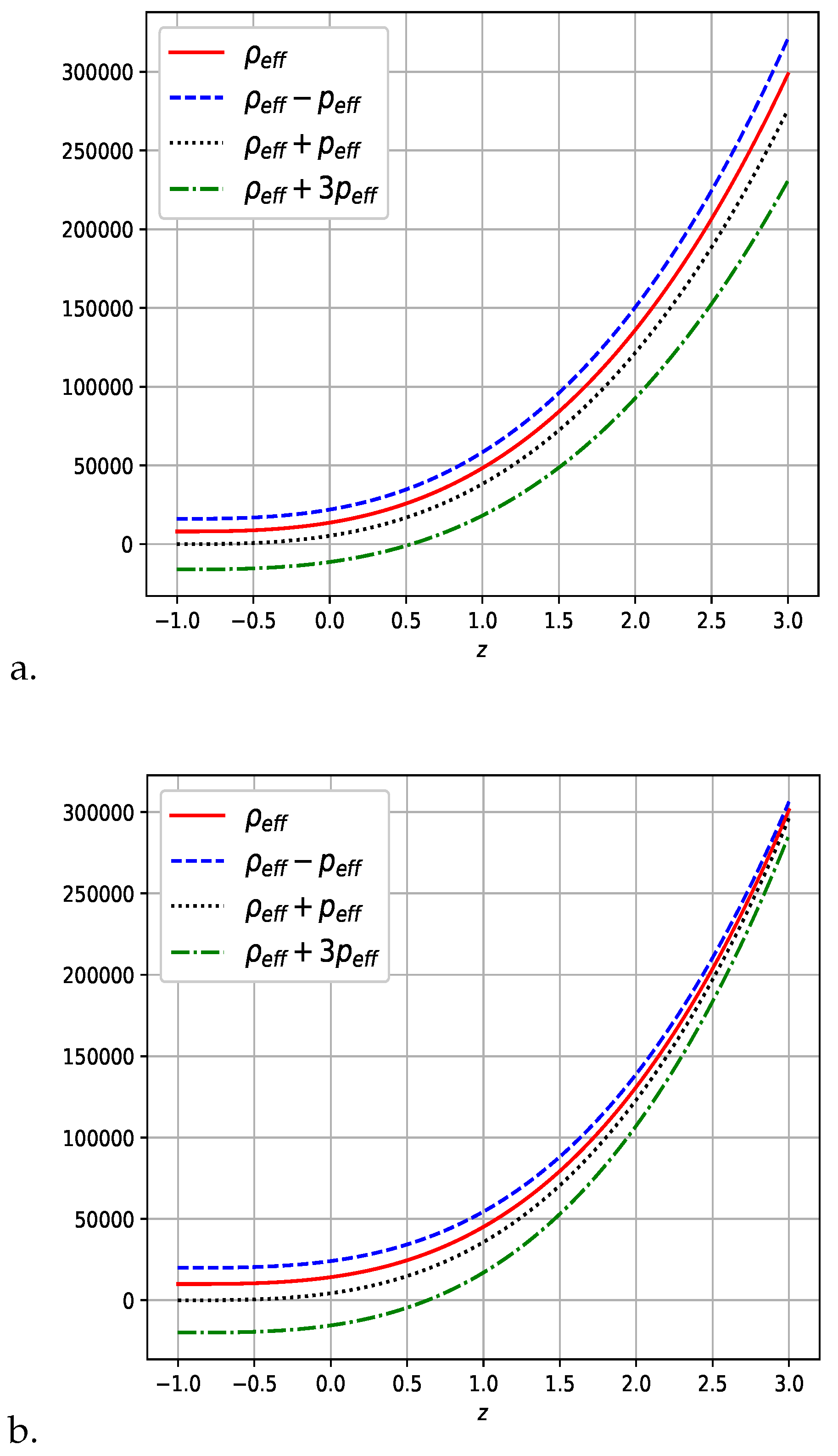
Figures 5a and 5b illustrate the progression of energy conditions as a function of z for the CC and CC+Pantheon datasets, respectively. It is evident that all energy conditions hold, except for the strong energy condition (SEC) when . The breakdown of SEC in this range is responsible for the accelerated expansion of the universe.
6.1. Om Diagnostic
The Om diagnostic function helps us classify theories about cosmic dark energy based on their behavior. We define the Om diagnostic function for a spatially homogeneous universe.
In this context, represents the present-day Hubble parameter, while corresponds to the Hubble parameter as defined in Eq. (37). When the function exhibits a positive slope, it indicates phantom-like behavior, whereas a negative slope signifies quintessence-like motion. The LambdaCDM model is characterized by a constant .
Equation shows the function for the model we developed, and Figure 6 illustrates its geometric meaning. Figure 6 shows that increases as z increases, indicating a positive slope. This suggests that our universe model behaves similarly to a phantom dark energy model. Also, we can see that as at late-time future, the value of is constant, which represents the tendency of our derived model to the CDM model in the far future.
7. Age of the Universe
We use the following formula to calculate the age of the universe as given below:
From Eq. (54), one can see that as , , then , which gives the present age of the universe. For the CC dataset, we estimate the age of the universe at Gyrs, and for the CC+Pantheon dataset, we get the age of the universe at Gyrs.
8. Conclusions
This paper presents the development of dark energy models within the framework of Weyl-type gravity, utilizing a dust fluid as the background source and taking into account relevant observational constraints. An analytical solution is derived for the field equations. The current values of the model parameters , , , , , m, and are determined through an analysis of data on the Hubble parameter sourced from cosmic chronometers, alongside brightness measurements obtained from the Pantheon sample of type Ia supernovae. The model’s physical properties are analyzed through the application of estimated values for its parameters, particularly focusing on the effective equation of state, , and the deceleration parameter, . The primary characteristics of the derived universe model are outlined as follows:
- We identified a transit phase characterized by deceleration in the past and acceleration in the late time, exhibiting phantom behavior in the dark energy model, which aligns well with recent observations.
- We found the Hubble constant value as Km/s/Mpc, along with CC data, and Km/s/Mpc along with joint data CC+Pantheon.
- We found the matter energy density parameter value as , and effective EoS parameter with dark energy EoS parameter as along CC data and along joint data CC+Pantheon which are in good agreement with recent observations.
- We looked into the model parameters , , m, and that are non-vanishing. These show how different factors affect the Weyl-type gravity theory.
- We found that the current value of the deceleration parameter is along the CC data and along the joint data CC+Pantheon. Both of these values are negative , which means that the universe model is speeding up right now.
- The current age of the universe is determined to be billion years based on the CC dataset. When incorporating both the CC and Pantheon datasets, the estimated age is refined to billion years.
- We found that our derived model satisfied all energy conditions except SEC which produces accelerating phase of the expanding universe.
- The Om diagnostic analysis reveals the phantom dark energy behavior of the model.
We see that the Weyl-type gravity theory could explain both the universe’s recent acceleration and its earlier slowing down without needing to add the cosmological constant . Therefore, the Weyl-type gravity needs more investigation to explore the properties of universe evolution.
Acknowledgments
The Inter-University Centre for Astronomy and Astrophysics (IUCAA), Pune, India, is acknowledged by the authors (A. Pradhan & A. Dixit) for its assistance through visiting associateship programs.
References
- S. Perlmutter, G. Aldering, G. Goldhaber, et al., Measurements of Omega and Lambda from 42 High-Redshift Supernovae, Astrophys. J. 517 (1999) 565-586, [arXiv:astro-ph/9812133].
- A. G. Riess, A. V. Filippenko, P. Challis, et al., Observational evidence from supernovae for an accelerating universe and a cosmological constant, Astron. J. 116 (1998) 1009-1038, [arXiv:astro-ph/9805201].
- A.G. Riess et al., Type Ia Supernova Discoveries at z > 1 from the Hubble Space Telescope: Evidence for Past Deceleration and Constraints on Dark Energy Evolution*. Astophys. J. 2004, 607, 665–687. [CrossRef]
- S. Hanany et al., MAXIMA-1: A Measurement of the Cosmic Microwave Background Anisotropy on angular scales of 10 arcminutes to 5 degrees, Astrophys. J, 545, L5 (2000).
- D.N. Spergel et al., Three-Year Wilkinson Microwave Anisotropy Probe (WMAP) Observations: Implications for Cosmology, Astrophys. J Suppl., 170, 377 (2007).
- E. Komatsu et al., Seven-year Wilkinson Microwave Anisotropy Probe (WMAP*) Observations: Cosmological Interpretation, Astrophys. J. Suppl., 192, 18 (2011).
- D.J. Eisenstein et al., Detection of the Baryon Acoustic Peak in the Large-Scale Correlation Function of SDSS Luminous Red Galaxies, Astrophys. J., 633, 560-574 (2005).
- H.A. Buchdahl, Non-Linear Lagrangians and Cosmological Theory, Mon. Not. R. Astron. Soc., 150, 1 (1970).
- T. Harko, F.S.N. Lobo, S. Nojiri, S.D. Odintsov, f(R,T) gravity. Phys. Rev. D 2011, 84, 024020.
- Cai, Yi-Fu and Capozziello, Salvatore and De Laurentis, Mariafelicia and Saridakis, Emmanuel N, f(T) teleparallel gravity and cosmology, Rep. Prog. Phys. 79(10) 106901 (2016). arXiv:1511.07586 [gr-qc].
- R. Ferraro, F. Fiorini, Modified teleparallel gravity: Inflation without an inflaton, Phys. Rev. D, 75, 084031 (2007).
- R. Myrzakulov, Accelerating universe from F(T) gravity, Eur. Phys. J. C, 71, 1752 (2011).
- S. Capozziello, V. F. Cardone, H. Farajollahi, A. Ravanpak, Cosmography in f(T) gravity, Phys. Rev. D, 84, 043527 (2011).
- J.B. Jimenez, L. Heisenberg, T. Koivisto, Coincident general relativity, Phys. Rev. D, 98, 044048 (2018).
- J. M. Nester and H. J. Yo, Symmetric teleparallel general relativity, Chin. J. Phys. 37 (1999) 113.
- Y. Xu, G. Li, T. Harko and S. D. Liang, f(Q,T) gravity, Eur. Phys. J. C 79 (2019) 708.
- S. Arora, S.K.J. Pacif, S. Bhattacharjee, f(Q,T) gravity models with observational constraints, P.K. Sahoo, Phys. Dark Univ., 30, 100664 (2020).
- S. Arora, A. Parida, P.K. Sahoo, Constraining effective equation of state in f(Q,T) gravity. Eur. Phys. J. C 2021, 81, 555. [CrossRef]
- R. Zia, D.C. Maurya, A.K. Shukla, Transit cosmological models in modified F(Q,T) gravity, Int. J. Geom. Meth. Mod. Phys., 18(04) 2150051 (2021). [CrossRef]
- E. Alvarez, S. Gonzalez-Martin, Weyl gravity revisited, J. Cosmol. Astropart. Phys., 02, 011 (2017).
- C. Gomes, O. Bertolami, Nonminimally coupled Weyl gravity, Class. Quantum Grav. 2019, 36, 235016. [CrossRef]
- Y. Xu, T. Harko, S. Shahidi, et al., Weyl type f(Q,T) gravity, and its cosmological implications, Eur. Phys. J. C 80 449 (2020). [CrossRef]
- J-Z. Yang, S. Shahidi, T. Harko, S-D. Liang, Geodesic deviation, Raychaudhuri equation, Newtonian limit, and tidal forces in Weyl-type f(Q,T) gravity, Eur. Phys. J. C, 81, 111 (2021).
- G. Gadbail, S. Arora, P.K. Sahoo, Power-law cosmology in Weyl-type f(Q,T) gravity, Eur. Phys. J. Plus, 136(10), 1040 (2021).
- J. T. Wheeler, Weyl gravity as general relativity, Phys. Rev. D, 90, 025027 (2014).
- R. Bhagat, S.A. Narawade, B. Mishra, Weyl type f(Q,T) gravity observational constrained cosmological models, Phys. Dark Univ. 41 (2023) 101250.
- G.N. Gadbail, S. Arora, P.K. Sahoo, Viscous cosmology in the Weyl-type f(Q,T) gravity. Eur. Phys. J. C 2021, 81, 1088. [CrossRef]
- M. Koussour, A model-independent method with phantom divide line crossing in Weyl-type f(Q,T) gravity, Chinese J. Phys. 83 (2023) 454-466.
- A.H.A. Alfedeel, M. Koussour, N. Myrzakulov, Probing Weyl-type f(Q,T) gravity: Cosmological implications and constraints, Astronomy and Computing 47 (2024) 100821.
- G. N. Gadbail, S. Arora, P. Kumar, P.K. Sahoo, Interaction of divergence-free deceleration parameter in Weyl-type f(Q,T) gravity. Chinese J. Phys. 2022, 79, 246–255. [CrossRef]
- E. J. Copeland, M. Sami and S. Tsujikawa, Dynamics of dark energy, Int. J. Mod. Phys. D 15, 1753 (2006), [arXiv:hep-th/0603057].
- J. Simon, L. Verde, R. Jimenez, Constraints on the redshift dependence of the dark energy potential, Phys. Rev. D 71, 123001 (2005).
- G. S. Sharov, V. O. Vasiliev, How predictions of cosmological models depend on Hubble parameter data sets, Math. Model. Geom. 6, 1-20 (2018).
- K. Asvesta, L. Kazantzidis, L. Perivolaropoulos, C.G. Tsagas, Observational constraints on the deceleration parameter in a tilted universe. Mon. Not. R. Astron. Soc. 2022, 513, 2394–2406. [CrossRef]
- D.W. Hogg and D.F. Mackey, Data analysis recipes: Using Markov Chain Monte Carlo, The Astrophysical Journal Supplement Series 236 (2018) 18. [arXiv:1710.06068 [astro-ph.IM]].
- R. Jimenez and A. Loeb, Constraining Cosmological Parameters Based on Relative Galaxy Ages, ApJ 573 (2002) 37.
- G. Ellis, R. Maartens, M. MacCallum, Relativistic Cosmology (Cambridge University Press, Cambridge, 2012). [CrossRef]
- A. Conley et al., Supernova constrants and systemetic uncertainities from the first three years of the supernova legacy survey*, ApJ 192 (2011) 1.
- D. M. Scolnic et al., The Complete Light-curve Sample of Spectroscopically Confirmed SNe Ia from Pan-STARRS1 and Cosmological Constraints from the Combined Pantheon Sample, ApJ 859 (2018) 101.
- Dong Zhao, Yong Zhou, Zhe Chang, Anisotropy of the Universe via the Pantheon supernovae sample revisited, MNRS 486 (2019) 5679-5689.
- L. Kazantzidis, L. Perivolaropoulos, Hints of a local matter underdensity or modified gravity in the low z Pantheon data. Phys. Rev. D 2020, 102, 023520. [CrossRef]
- D. Sapone, et al., Is there any measurable redshift dependence on the SN Ia absolute magnitude? Phys. Dark Univ. 2021, 32, 100814. [CrossRef]
- L. Kazantzidis, H. Koo, S. Nesseris, L. Perivolaropoulos, A. Shafieloo, Hints for possible low redshift oscillation around the best-fitting ΛCDM model in the expansion history of the Universe, MNRS 501 (2021) 3421-3426.
- M. G. Dainotti et al., On the Hubble Constant Tension in the SNe Ia Pantheon Sample, ApJ 912 (2021) 150.
- M. G. Dainotti et al., On the Evolution of the Hubble Constant with the SNe Ia Pantheon Sample and Baryon Acoustic Oscillations: A Feasibility Study for GRB-Cosmology in 2030. Galaxies 2022, 10, 24. [CrossRef]
- G. Alestas, L. Kazantzidis, L. Perivolaropoulos, w-M phantom transition at zt≃0.1 as a resolution of the Hubble tension. Phys. Rev. D 2021, 103, 083517. [CrossRef]
- D. Camarena, V. Marra, On the use of the local prior on the absolute magnitude of Type Ia supernovae in cosmological inference, MNRS 504 (2021) 5164-5171.
- V. Marra, L. Perivolaropoulos, Rapid transition of Geff at zt≃0.01 as a possible solution of the Hubble and growth tensions. Phys. Rev. D 2021, 104, L021303. [CrossRef]
- G. Alestas, I. Antoniou L. Perivolaropoulos, Hints for a Gravitational Transition in Tully-Fisher Data, Universe 7 (2021) 366. [CrossRef]
- L. Perivolaropoulos, Is the Hubble crisis connected with the extinction of dinosaurs?, arXiv:2201.08997 [astro-ph.EP].
- D. C. Maurya, Late-time accelerating cosmological models in f(R,Lm,T)-gravity with observational constraints. Phys. Dark Universe 2024, 46, 101722. [CrossRef]
- D. C. Maurya, K. Yesmakhanova, R. Myrzakulov, G. Nugmanova, FLRW Cosmology in Metric-Affine F(R,Q) Gravity, Chinese Phys. C 48(12) 125101 (2024).
- D. C. Maurya, Transit dark energy models in Hoyle-Narlikar gravity with observational constraints. Phys. Dark Univ. 2025, 47, 101782. [CrossRef]
- D. C. Maurya, Constrained transit cosmological models in f(R,Lm,T)-gravity, Int. J. Geom. Meth. Mod. Phys. 2025. [CrossRef]
- D. C. Maurya, Accelerating cosmological models in Hoyle-Narlikar gravity with observational constraints, Int. J. Geom. Meth. Mod. Phys., (2025). [CrossRef]
- A.R. Lalke, G.P. Singh, A. Singh, Cosmic dynamics with late-time constraints on the parametric deceleration parameter model. Eur. Phys. J. Plus 2024, 139, 288. [CrossRef]
- S. Mandal, A. Singh, R. Chaubey, Late-time constraints on barotropic fluid cosmology. Phys. Lett. A 2024, 519, 129714. [CrossRef]
- A. Singh, S. Krishnannair, Affine EoS cosmologies: Observational and dynamical system constraints. Astronomy and Computing 2024, 47, 100827. [CrossRef]
- S. Capozziello, O. Farooq, O. Luongo, et al., Cosmographic bounds on the cosmological deceleration-acceleration transition redshift in f(R) gravity, Phys. Rev. D 90, 044016 (2014), [arXiv:1403.1421v1 [gr-qc]].
- S. Capozziello, O. Luongo, E. N. Saridakis, Transition redshift in f(T) cosmology and observational constraints, Phys. Rev. D 91 124037 (2015), [arXiv:1503.02832v2 [gr-qc]].
- S. Capozziello, P. K. S. Dunsby, O. Luongo, Model independent reconstruction of cosmological accelerated-decelerated phase, MNRAS 509 (2022) 5399-5415, [arXiv:2106.15579v2 [astro-ph.CO]].
- M. Muccino, O. Luongo, D. Jain, Constraints on the transition redshift from the calibrated Gamma-ray Burst Ep-Eiso correlation, MNRAS 523 (2023) 4938-4948, [arXiv:2208.13700v3 [astro-ph.CO]].
- A. C. Alfano, S. Capozziello, O. Luongo, et al., Cosmological transition epoch from gamma-ray burst correlations, (2024) [arXiv:2402.18967v1 [astro-ph.CO]].
- A. C. Alfano, C. Cafaro, S. Capozziello, et al., Dark energy-matter equivalence by the evolution of cosmic equation of state, Phys. Dark Univ. 42 101298 (2023), [arXiv:2306.08396v2 [astro-ph.CO]].
- M. Sharif and A. Ikram, Energy conditions in f(G,T) gravity, Eur. Phys. J. C 76 (2016) 640. arXiv:1608.01182v3 [gr-qc].
- S. Carroll, Spacetime and Geometry: An Introduction to General Relativity, Addison Wesley (2004).
- R. Schoen and S. T. Yau, Proof of the positive mass theorem. II. Commun. Math. Phys. 1981, 79, 231. [CrossRef]
- S. W. Hawking and G. F. R. Ellis, The Large Scale Structure of Space-time, Cambridge University Press, (1973).
- V. Sahni, A. Shafieloo, A. A. Starobinsky, Two new diagnostics of dark energy. Phys. Rev. D 2008, 78, 103502. [CrossRef]
Figure 3.
Variation of effective EoS parameter and dark energy EoS parameter over z.
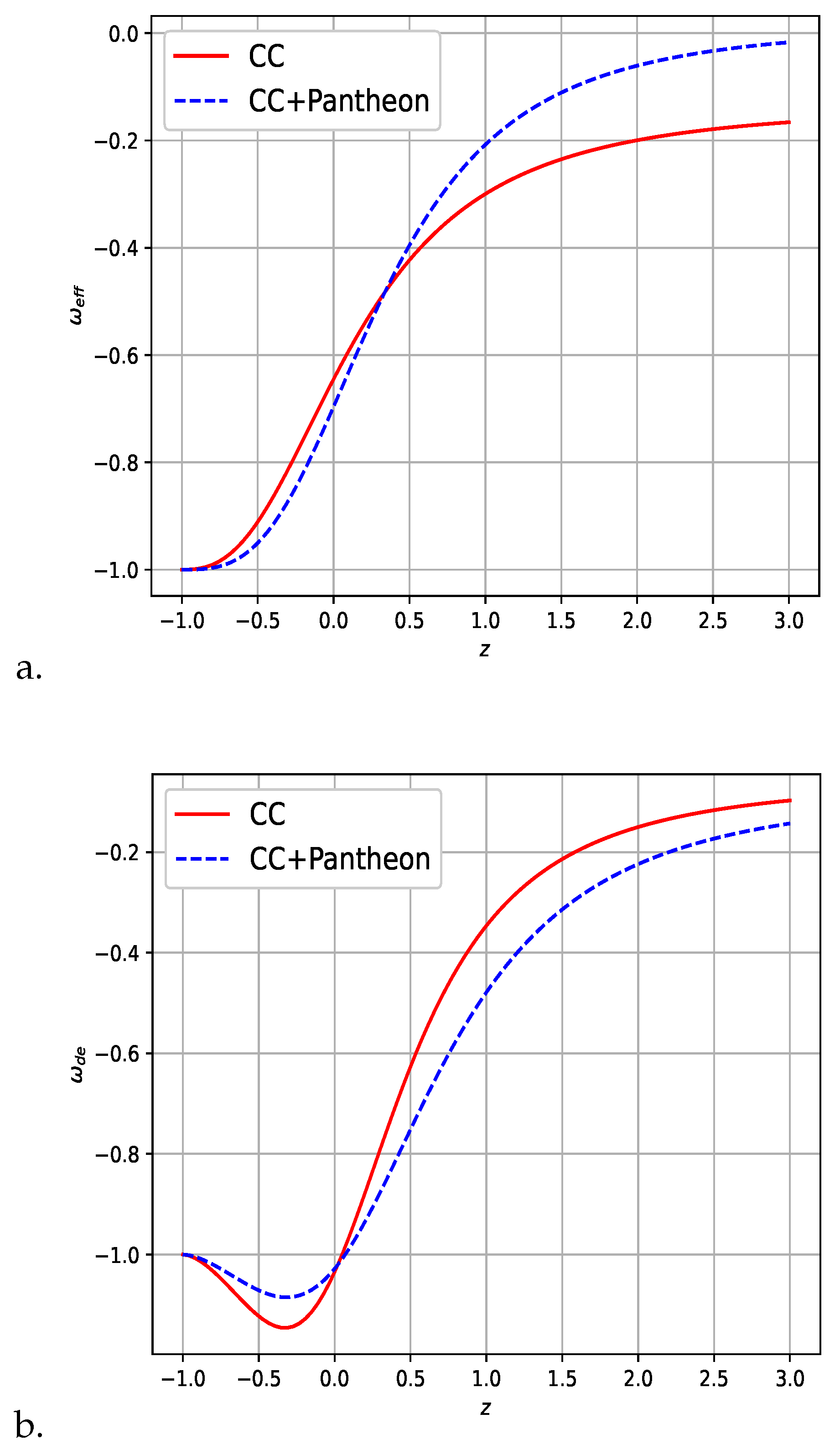
Figure 4.
Evolution of deceleration parameter versus z.

Figure 6.
Behaviour of the over z.
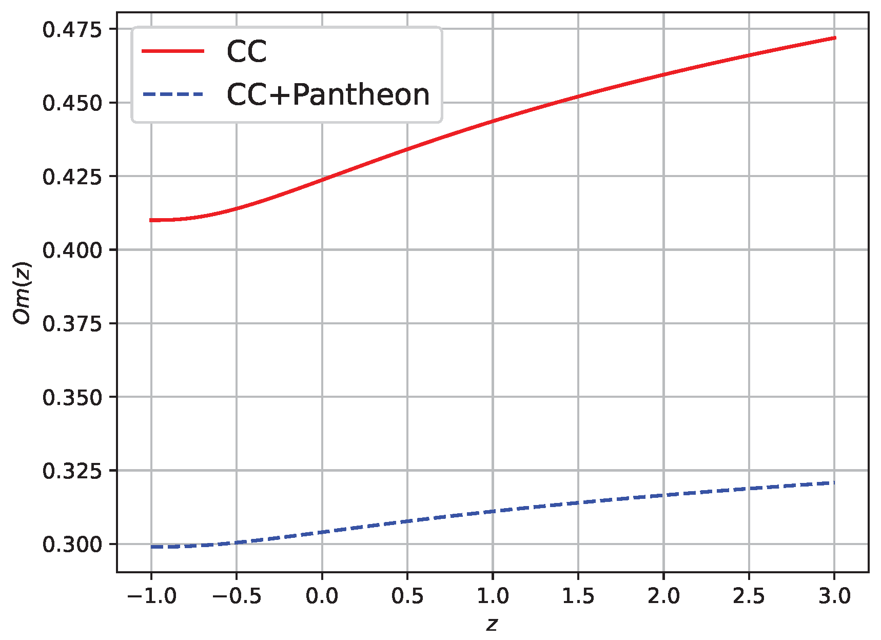

Table 1.
The MCMC estimates.
| Parameter | Prior | CC | CC+Pantheon |
|---|---|---|---|
| - | |||
| - |
Disclaimer/Publisher’s Note: The statements, opinions and data contained in all publications are solely those of the individual author(s) and contributor(s) and not of MDPI and/or the editor(s). MDPI and/or the editor(s) disclaim responsibility for any injury to people or property resulting from any ideas, methods, instructions or products referred to in the content. |
© 2025 by the authors. Licensee MDPI, Basel, Switzerland. This article is an open access article distributed under the terms and conditions of the Creative Commons Attribution (CC BY) license (http://creativecommons.org/licenses/by/4.0/).
Copyright: This open access article is published under a Creative Commons CC BY 4.0 license, which permit the free download, distribution, and reuse, provided that the author and preprint are cited in any reuse.


