Submitted:
26 June 2025
Posted:
01 July 2025
Read the latest preprint version here
Abstract
Personalised modelling has become a dominant approach in personalised medicine and precision health. It creates a computational model for an individual, based on large data repositories of existing personalised data, aiming to achieve the best possible personal diagnosis or prognosis and derive an informative explanation for it. Current methods are still working on a single data modality or treating all modalities with the same method. The proposed method, SAIN (Search-And-INfer), offers better results and an informative explanation for classification and prediction tasks on a new multimodal object (sample) using a database of similar multimodal objects. The method is based on different distance measures suitable for each data modality and introduces a new formula to aggregate all modalities into a single vector distance measure to find the closest objects to a new one and then use them for a probabilistic inference. The paper describes SAIN and applies it to two types of multimodal data, cardiovascular diagnosis and EEG time series, modelled by integrating modalities, such as numbers, categories, images, and time series, and using a software implementation of SAIN. The method offers personalised explainability for medical diagnosis or prognosis. . 12 search in multimodal data; inference in multimodal data; personalised modelling; precision health.
Keywords:
search in multimodal data
; inference in multimodal data
; personalised modelling
; precision health
1. Introduction
Multimodal data processing has become a new data science trend with applications in neuro-imaging, health diagnosis and prognosis, environmental modeling, and financial modelling, see [1,2,3].
Methods for searching relevant items in databases have been developed and used for decades, improving their accuracy and speed. These searches are a significant part of personalised modelling (e.g. precision medicine), where an optimal model is created for a given vector of person x data X and a database D of past personalised records with labelled outcomes to predict x behaviour. Most methods (e.g. [3,4]) select a subset of closest vectors to X from the database D (for example, the K-nearest neighbours) and build a machine learning model using this subset . To select a subset of the closest vectors to X, the method searches D using predominantly Euclidean or Hamming distances to measure the similarity between the new vector X and the vectors in D. These methods have been applied in many applications and constitute the state-of-the-art in the field (e.g. [5,6,7,8]).
The enormous growth of personal multimodal data worldwide demands more advanced personalisation of search and inference methods. Most methods for multi-modal data represent all modalities of data for one object as a vector and then apply a single machine learning method, such as a deep neural network or a statistical regression (e.g. [9,10]). In these cases, the specificity of each data modality cannot be considered, which negatively impacts the inference results and explanation.
The proposed new method offers new functionality and features for personalised search and model creation in multimodal data, some of which are listed below. The method
- is suitable for multimodal data searches in heterogeneous data sets, e.g. numbers, text, images, sound, and categorical data,
- uses a novel mathematical similarity measure superseding a single (e.g. Euclidean, Hamming) distance used in the existing methods. In this way, inaccurate measurement of similarity on a large number of heterogeneous variables is avoided,
- search is fast even on large data sets, with millions of records and thousands of variables,
- includes advanced personalised searches with multiple parameters and other features,
- facilitates multiple solutions with corresponding probabilities,
- is suitable for unsupervised clustering in multimodal heterogeneous data,
- is suitable for personalised model creation to classify or predict specific outcomes based on multimodal and heterogeneous data.
2. Mathematical Description
In this section, we present the mathematical method.
2.1. Database
We will work with the multidimensional data described as follows:
- objects (samples) ,
- each object () is defined by criteria (variables) with values in linearly ordered domains with and ; if some value (, ) is either missing or uncertain, then its value is recorded as ∞,
- weights in with , where each () quantifies the importance of the criterion ; if for all , then all criteria are equally important; a criterion is ignore if .
Data of independent variables are organised as follows:

Table 1.
Unlabelled database.
| Objects/Criteria | ... | ... | ||||
| ... | ... | |||||
| ⋮ | ⋮ | ⋮ | ... | ⋮ | ... | ⋮ |
| ... | ... | |||||
| ⋮ | ⋮ | ⋮ | ... | ⋮ | ... | ⋮ |
| ... | ... | |||||
| w | ... | ... |
2.2. Distance Metrics
A distance metric on a space X is a positive real-valued function satisfying the following three conditions for all : a) if and only if , b) , c) .
The domains can vary greatly: they can be sets of logical values, rational numbers, percentages, digitally codified images, sounds, videos, and many others. We use a bounded distributive complemented lattice to describe uniformly the domains , [11,12].
Here is a list with illustrative, but far from exhaustive, examples of domains :
- Logical Boolean domain: , where .
- Logical non-Boolean domain: , where and .
- Numerical domain with natural values: , where .
- Numerical domain with rational values: , where .
- Binary code: , where the domain consists of all binary strings of length n, and for all , , ,
In the lattice we introduce, following [11], the metric:
for . This metric d can be extended to as follows:
where .
The metrics on , , can be extended to , i.e. to n-dimensional vectors, as follows:
where , .
In what follows, we write d for when the meaning is clear from the context.
2.3. Tasks Specification
Data organised as in Table 2 consists of independent objects augmented with a column of labels, the weights of criteria, and a new unlabelled object, see Table 2 and Table 3.
Additional information associated with data in Table 2 may include the range of each criterion and the associated specific distance, e.g. the Euclidean distance for real numbers and the distance d for binary strings or strings over a non-binary alphabet (e.g. for images or colours).
We consider the following tasks:
- Task
- 1: Calculate the distance (or similarity metric) between the new object and each object in Table 2. If the distance corresponding to is , then
- Task
- 2: Given a threshold , calculate all objects at a distance at most to x.
- Task
- 3: Calculate the probability of a new object to belong to a labelled class (e.g. low risk vs. high risk) using a threshold and Table 2.
- Task
- 4: Rank the criteria in Table 2 and calculate the marker or markers criterion/criteria, that is the most important one/ones.
- Task
- 5: Assign alternative weights to criteria.
- Task
- 6: Test the accuracy of data and method for Task 4.
2.4. Tasks Solutions
For Task 2, given a threshold , we calculate all objects in Table 2 at a distance at most to x, that is, the objects which are -similar to x:
and its complement .
For Task 3 we calculate the probability that x is in class label , which is the ratio of the number of objects in with the label to the size of the cluster :
where means the number of elements in the set .
For Task 4, we work with Table 2. Recall that for each criterion we have a domain augmented with information “high" or “low," indicating whether higher or lower values are desirable. Based on this information, we can construct a hypothetical object which has as the most desirable values for each criterion: one could see this object as an “exemplar" one.
Table 5.
Hypothetical exemplar object.
| Object/Criteria | ... | ... | Class label | ||||
| ... | ... |
Sometimes, criteria are interrelated or correlated. This means that in some cases, there is no unique “exemplar object", but a couple of them have to be studied in ranking the importance of criteria.
For example, fix an “exemplar object" .
- Compute the distances between each object in Table 2 and , so obtain a vector with n non-negative real components .
- For each , compute the distances taking into consideration all criteria in Table 2except: obtain the vector .
- Compute the distances between , using the formulaand sort them in increasing order. The criterion is a marker if , for every .
We repeat this procedure for each “exemplar object" and study possible variations.
For Task 5, normalise the distances and use these values to construct the weights , .
2.5. An Example
We illustrate the above tasks with an example of a labelled database in (see Table 6) and a new object (see Table 7), all having the following seven characteristics (the last column has the label classes 1 and 2):
- : real number , e.g. age, weight, BMI etc.;
- : Boolean value , e.g. gender;
- : integer number , e.g. gene expression;
- : categorical {small, med, large }, e.g. size of tumour, body size, keywords;
- : colour {red, yellow, white, black}, e.g. colour of a spot on the body, on the heart;
- : spike sequence of e.g. encoded EEG, ECG;
- : black and white image, e.g. MRI, face image.
In this example, for simplicity, we didn’t use weights.
Then, we normalise the data in Table 8 and Table 9 – the entries in the first, third and fourth columns have been divided by 100, 10,000 and 2, respectively, and the entries in the last three columns have been transformed in reals in the unit interval, and the column of labels has been removed.
Then, we choose an appropriate distance according to each criterion. In this example, we used the Euclidean distance for all criteria.
We can compute and, accordingly, the probability that x would be labelled in class 1 or class 2.
If , then so the probability that x is in class 1 is 2/7 and the probability that x is in class 2 is 5/7. If , then its closest cluster is , so the probability that x is in class 1 is 1/3 and the probability that x is in class 2 is 2/3.
Table 12.
Normalised distances from the new object to all objects.
| 0.197 | 1 | 0.3889 | 1 | 0 | 0.4 | 0.11111111 | 3.09701111 | |
| 0.445 | 0 | 0.52321 | 0.5 | 0.33333333 | 0.6 | 0.22222222 | 2.62376556 | |
| 0.04 | 0 | 0.40079 | 0 | 0 | 0.5 | 0.22222222 | 1.16301222 | |
| 0.083 | 1 | 0.4559 | 1 | 0.66666667 | 0.45 | 0.11111111 | 3.76667778 | |
| 0.222 | 1 | 0.36223 | 0 | 0.33333333 | 0.45 | 0.22222222 | 2.58978556 | |
| 0.33 | 0 | 0.33276 | 0.5 | 0 | 0.45 | 0.11111111 | 1.72387111 | |
| 0.082 | 0 | 0.23221 | 1 | 0.33333333 | 0.45 | 0.22222222 | 2.31976556 | |
| 0.285 | 1 | 0.37846 | 0 | 0.33333333 | 0.45 | 0.22222222 | 2.66901556 | |
| 0.285 | 1 | 0.37846 | 1 | 0.33333333 | 0.45 | 0.22222222 | 3.66901556 |
Table 13.
Ranking of distances in increasing order in Table 12.
Table 13.
Ranking of distances in increasing order in Table 12.
| 0.04 | 0 | 0.40079 | 0 | 0 | 0.5 | 0.22222222 | 1.16301222 | |
| 0.33 | 0 | 0.33276 | 0.5 | 0 | 0.45 | 0.11111111 | 1.72387111 | |
| 0.082 | 0 | 0.23221 | 1 | 0.33333333 | 0.45 | 0.22222222 | 2.31976556 | |
| 0.222 | 1 | 0.36223 | 0 | 0.33333333 | 0.45 | 0.22222222 | 2.58978556 | |
| 0.445 | 0 | 0.52321 | 0.5 | 0.33333333 | 0.6 | 0.22222222 | 2.62376556 | |
| 0.285 | 1 | 0.37846 | 0 | 0.33333333 | 0.45 | 0.22222222 | 2.66901556 | |
| 0.197 | 1 | 0.3889 | 1 | 0 | 0.4 | 0.11111111 | 3.09701111 | |
| 0.285 | 1 | 0.37846 | 1 | 0.33333333 | 0.45 | 0.22222222 | 3.66901556 | |
| 0.083 | 1 | 0.4559 | 1 | 0.66666667 | 0.45 | 0.11111111 | 3.76667778 |
which induces a ranking of the objects in the Table 8: .
For Task 4, assume that the criteria in Table 10 have the additional information , where m (M) means that the exemplar value is the minim (maximum) value. Based on this vector, we compute the exemplar object:
Table 14.
Exemplar object.
| 0.2 | 0 | 0.00089 | 0 | 1 | 0.1222210012 | 0.100001001 |
Next we calculate , see Table 14, and finally the distances , and the weights as their normalised values, see Table 16. The marker, in this case, is the criterion .
Table 15.
Vectors , rounded to two decimals.
| 1.469 | 0.987 | 1.469 | 1.402 | 1.469 | 0.669 | 1.359 | 1.459 |
| 3.709 | 2.979 | 2.709 | 2.730 | 3.209 | 3.309 | 3.609 | 3.709 |
| 3.220 | 2.975 | 2.220 | 3.165 | 2.220 | 2.420 | 3.110 | 3.210 |
| 0.378 | 0.010 | 0.378 | 0.378 | 0.378 | 0.378 | 0.378 | 0.368 |
| 2.167 | 2.104 | 2.167 | 2.073 | 1.167 | 1.167 | 2.167 | 2.157 |
| 3.824 | 3.209 | 2.824 | 3.035 | 3.324 | 3.024 | 3.714 | 3.814 |
| 3.066 | 2.699 | 2.066 | 2.378 | 3.066 | 2.066 | 3.066 | 3.055 |
| 1.487 | 1.487 | 1.487 | 1.410 | 0.487 | 1.087 | 1.477 | 1.487 |
| 1.487 | 1.487 | 1.487 | 1.410 | 0.487 | 1.087 | 1.477 | 1.487 |
Table 16.
Distances and (normalised) weights.
| Distances | 2.870 | 4.00 | 2.826 | 5.00 | 5.60 | 0.450 | 0.061 |
| Weights | 0.137 | 0.192 | 0.135 | 0.240 | 0.269 | 0.021 | 0.002 |
3. Survival Analysis in SAIN
Medical survival analysis evaluates the time until an event of interest occurs, like death or disease recurrence, in a group of patients. This analysis is often used to compare treatment outcomes or predict prognosis.
3.1. Data and Tasks
We are given the following data:
- Table 17 in which the first column lists the patients treated for the same disease with the same method under strict conditions and the last column records the times till the patient’s deaths.
- Table 18, which includes the record of the new patient p.
- A threshold which defines the acceptable similarity between p and the relevant ’s in the Survival database (i.e. ).
We consider the following tasks:
Task 1: What is the life expectancy of p?
Task 2: What is the probability that the life expectancy of p is greater than or equal to a given T?
3.2. Tasks Solutions
Using a standard method of survival analysis
-
For Task 1,
- (a)
- Compute the set of patients that are similar up to to p:
- (b)
- Using , compute the probability that p will survive the time :
- (c)
- Compute the life expectancy of p using the formula:
- For Task 2, calculate the probability that the life expectancy of p is at least time T:
3.3. An Example
We illustrate the above tasks with an example of a database in which columns 2–8 record patients’ medical test results, and the last column records time to death (see Table prec) and a new patient (see Table 20):
Table 19.
Patient records.
| patients | units of time | |||||||
| 0.682 | 0 | 0.06789 | 0 | 0.2 | 0.012211001 | 0.110001001 | 12.3 | |
| 0.93 | 1 | 0.98 | 0.5 | 0.6 | 0.022220012 | 0.100001001 | 15 | |
| 0.445 | 1 | 0.056 | 1 | 0.2 | 0.012121001 | 0.110101111 | 68 | |
| 0.568 | 0 | 0.00089 | 0 | 1 | 0.122221001 | 0.110011101 | 1.4 | |
| 0.263 | 0 | 0.09456 | 1 | 0 | 0.122201001 | 0.110111101 | 40.5 | |
| 0.815 | 1 | 0.78955 | 0.5 | 0.2 | 0.012122001 | 0.110001111 | 97.2 | |
| 0.567 | 1 | 0.689 | 0 | 0 | 0.122121001 | 0.111001111 | 97.2 | |
| 0.2 | 0 | 0.07833 | 1 | 0.6 | 0.112211022 | 0.100001111 | 55.7 | |
| 0.2 | 0 | 0.07833 | ∞ | 0.6 | 0.112211022 | 0.100001111 | 63.7 |
Table 20.
New patient records.
| 0.485 | 1 | 0.45679 | 1 | 0.2 | 0.1002121001 | 0.110001101 |
The distance for column 4 is and . For example, . For all other columns, the distance is . Finally, the total distance is the sum of individual distances (7 terms), with the results in Table 21.
The results for Task 1, (a), (b) and (c) are listed below:
-
For , , that is the entire database. Then
- (a)
- ,
- (b)
- ,
- ,
- ,
- ,
- ,
- ,
- ,
- .
- (c)
- ,
- ,
- ,
- ,
- ,
- ,
- ,
- ,
We can calculate other probabilities, for example, . -
For , . Then
- (a)
- ,
- (b)
- ,
- ,
- ,
- ,
- ,
- (c)
- ,
- ,
- ,
- ,
- .
Similarly, we can calculate the probabilities , .
4. SAIN: A Modular Diagram and Functional Information Flow
5. Case Studies for Medical Diagnosis and Prognosis
We present three case studies in which we applied SAIN.
5.1. Heart Disease Diagnosis
We worked with the well-known Cleveland dataset, which contains multiple data types [13]. The UCI Heart Disease data set contains 76 attributes. As in most articles, the attributes in our experiment data were restricted to 14, see Table 22.
The problem is a binary classification on whether the patient has or does not have heart disease.
First, we selected suitable distance metrics and weights to classify the attributes. For binary objects, the distance metric is simply whether they are equal; for non-binary discrete objects such as resting electrocardiographic results, the appropriate distance measure is not obvious and should be informed by an expert. We give electrocardiographic results 0 for normal, 1 for having ST-T wave abnormality, and 2 for showing probable or definite left ventricular hypertrophy following Estes’ criteria.
Many studies with the Cleveland dataset have been tested with different machine learning techniques. For example, [14] lists different algorithms and performances ranging from 47% to 80% accuracy. SAIN achieved an 82% accuracy score. Why SAIN? The search is fast, it uses appropriate distances chosen by a medical expert, it provides explainability at a personal level including probabilities. If offers different scenarious for modelling by experimenting different sets of features, parameters and preferred outcome vizualitations.
5.2. Time Series Classification
Many data sets for classifying outcomes of events consist of multiple time series. Each variable in a time series may depend on other variables that change in time. The proposed model can deal with this problem by encoding time series (signal) into binary vectors which can be processed for classification in the SAIN framework. The variables for this data set are 14 channels of temporal EEG data channels, located at places of interest on the human scalp.
The signals measured over the same time period are the EEG channels, fMRI voxels, ECG electrodes, seismic sensory signals, financial time series, gene expressions, voice, and music frequency bands [8]. Even when the variable (signal) measurements are independent, the signals may have an impact on each other as they represent the same object/person at the same time period. The number N of these signals can vary from just a few for a short time window T (Figure 3) to hundreds and thousands when the time varies from a few milliseconds to minutes, hours, days, etc.
Next we present a simple example how this search can be computed for a new record X consisting of only 3 variables/signals (e.g. EEG channels, ECG electrodes) over a short period of 5 time moments and the data base D constituting of only 6 such records which are labelled by an outcome labels 1,2,3 (e.g. diagnosis, prognosis).
In addition to the record X, a weight vector is supplied with the weighted importance of the signals at different time points, e.g. , meaning that the most important and informative part of the measurements is at time point 3.
The new record (signal, EEG channel 1) 0, 1, 1, 1, -1 (signal, EEG channel 2) 1, 1, -1, -1, 0 (signal, EEG channel 3),
The database contains records where:
Table 23.
Caption.
| Record | Channel 1 | Channel 2 | Channel 3 | Label |
| R1 | (1, 1, -1, 0, 1) | (0, 1, 1, 1, -1) | (1, 1, -1, -1, 0) | 1 |
| R2 | (1, 0, -1, 0, 1) | ( 0, 1, 1, 1, -1) | (1, 0, -1, -1, 1 ) | 1 |
| R3 | (1, 1, -1, 0, 1) | (0, -1, 1, 1, -1) | (1, 1, -1, 0, 1) | 2 |
| R4 | (1, 1, -1, 0, 1) | (0, -1, 1, 0, -1) | (1, 1, -1, 0, 1) | 2 |
| R5 | (1, 1, -1, 0, 0) | (0, -1, 0, 1, -1) | (1, 1, -1, 1, 1) | 3 |
| R6 | (1, -1, -1, 0, 1) | (0, -1, 1, 0, -1) | (1, 1, -1, 0, 1) | 3 |
The new record X of EEG-signals will be classified in class 1 as it is closest according to the Euclidian distance class 1 data samples and .
5.3. Predicting Longevity in Cardiac Patients
We utilised a data set in which we applied a binary classification on whether the patient had an event (e.g. death) and further to those that had an event whether this would occur in the near future (within the next 180 days, e.g. approximately six months). The data set contained a set of 150 variables and an outcome, with 295 patients in the first data set and 49 in the second. The data included a mix of variables that could be grouped as follows:
- demographics, risk factors, disease states, medication and deprivation scores,
- echocardiography, cardiac ultrasound measurements,
- advanced ECG measurements,
The other data includes the days until the event occurred of the censor date for the Cox proportional hazard monitoring.
The objectives are to predict an arrhythmic event or death.
Before running the algorithm, the data was normalised, and to account for the data being unbalanced, we utilised SMOTE data balancing method [15] each time we left one out (ensuring that we did not SMOTE when the true data point was part of the data set). For the event classification data set, the model achieved an accuracy of 79%. This is broken down into classifying no event (198/247, 80%) and an event with (36/49, 73%) accuracy. It is worth noting the confidence of each individual could be explored with a sample of the confidence for classification in Figue Figure 6.
For the second experiment, we normalised the dataset and removed any columns with unknown values. We then applied a genetic algorithm to find the set of features to use for classification. We found a set of 34 variables which would provide an accuracy of with (34/34) for class 0 and (6/15) for class 1. Alternatively, we find that if we apply SMOTE and focus more on the accuracy of class 1, we obtain accuracy, however, more evenly distributed with (24/34) for class zero and (10/15) for class 1.
6. Data and Software Availability
The data has been obtained from the following: UCI Cleveland data available at https://archive.ics.uci.edu/dataset/45/heart+disease EEG data available at https://github.com/KEDRI-AUT/NeuCube-Py/tree/master/example_data Access to the software is available on request.
7. Conclusions
The paper presents a new method for search and inference, called here SAIN, for multi-modal data integration and personalised model creation based on these multi-modal data. The model not only evaluates the outcome for a person more accurately than traditional machine learning methods using a single modality data, but it also explains the proposed solution in terms of probability and visual explanation.
The proposed method is implemented as a computer system and applied to several case studies to illustrate its advantages and applicability. The SAIN method described in Section 4 was implemented as a software system.
The proposed mathematical method and computational framework can be applied to a broad spectrum of applications, such as [15]: a) medical diagnosis based on multimodal data, such as genetic, clinical, cognitive, and ethnical, b) early disease prognosis based on multimodal personalised data modelling, c) multimodal neuroimaging data modelling, d) multisensory spatio-temporal data modelling for pollution level estimation and prediction, e) earthquake prediction based on both seismic and GPS spatio-temporal data.
Acknowledgement
We thank Dr. Elena Calude for the contributions to the mathematical model.
References
- AbouHassan, I.; Kasabov, N.K.; Jagtap, V.; Kulkarni, P. Spiking neural networks for predictive and explainable modelling of multimodal streaming data with a case study on financial time series and online news. Sci. Rep. 2023, 13, 18367. [Google Scholar] [CrossRef] [PubMed]
- Rodrigues, F.; Markou, I.; Pereira, F.C. Combining time-series and textual data for taxi demand prediction in event areas: A deep learning approach. Information Fusion 2019, 49, 120–129. [Google Scholar] [CrossRef]
- Li, J.; Liu, J.; Zhou, S.; Zhang, Q.; Kasabov, N.K. GeSeNet: A General Semantic-Guided Network With Couple Mask Ensemble for Medical Image Fusion. IEEE Transactions on Neural Networks and Learning Systems 2024, 35, 16248–16261. [Google Scholar] [CrossRef] [PubMed]
- Kasabov, N. Data Analysis and Predictive Systems and Related Methodologies, U.S. Patent 9,002,682 B2, 7 April 2015. [Google Scholar]
- Doborjeh, M.; Doborjeh, Z.; Merkin, A.; Bahrami, H.; Sumich, A.; Krishnamurthi, R.; Medvedev, O.N.; Crook-Rumsey, M.; Morgan, C.; Kirk, I.; et al. Personalised predictive modelling with brain-inspired spiking neural networks of longitudinal MRI neuroimaging data and the case study of dementia. Neural Networks 2021, 144, 522–539. [Google Scholar] [CrossRef] [PubMed]
- Budhraja, S.; Singh, B.; Doborjeh, M.; Doborjeh, Z.; Tan, S.; Lai, E.; Goh, W.; Kasabov, N. Mosaic LSM: A Liquid State Machine Approach for Multimodal Longitudinal Data Analysis. In Proceedings of the 2023 International Joint Conference on Neural Networks (IJCNN). IEEE; 2023; pp. 1–8. [Google Scholar] [CrossRef]
- Kasabov, N.K. Evolving connectionist systems, 2 ed.; Springer: London, England, 2007. [Google Scholar]
- Kasabov, N.K. Time-Space, Spiking Neural Networks and Brain-Inspired Artificial Intelligence; Springer Berlin Heidelberg, 2019. [CrossRef]
- Santomauro, D.F.e.a. Global prevalence and burden of depressive and anxiety disorders in 204 countries and territories in 2020 due to the COVID-19 pandemic Global prevalence and burden of depressive and anxiety disorders in 204 countries and territories in 2020 due to the COVID-19 pandemic. The Lancet, 1700. [Google Scholar]
- Swaddiwudhipong, N.; Whiteside, D.J.; Hezemans, F.H.; Street, D.; Rowe, J.B.; Rittman, T. Pre-diagnostic cognitive and functional impairment in multiple sporadic neurodegenerative diseases. bioRxiv, 2022. [Google Scholar] [CrossRef]
- Calude, C.; Calude, E. A metrical method for multicriteria decision making. St. Cerc. Mat 1982, 34, 223–234. [Google Scholar]
- Calude, C.; Calude, E. On some discrete metrics. Bulletin mathématique de la Société des Sciences Mathématiques de la République Socialiste de Roumanie.
- Gleeson, S.; Liao, Y.W.; Dugo, C.; Cave, A.; Zhou, L.; Ayar, Z.; Christiansen, J.; Scott, T.; Dawson, L.; Gavin, A.; et al. ECG-derived spatial QRS-T angle is associated with ICD implantation, mortality and heart failure admissions in patients with LV systolic dysfunction. PLOS ONE 2017, 12, e0171069. [Google Scholar] [CrossRef] [PubMed]
- Kahramanli, H.; Allahverdi, N. Design of a hybrid system for the diabetes and heart diseases. Expert systems with applications 2008, 35, 82–89. [Google Scholar] [CrossRef]
- Kasabov, N.K. Time-space, Spiking Neural Networks and Brain-inspired Artificial Intelligence; Vol. 750, Springer, 2019.
Figure 1.
A modular diagram of the proposed SAIN computational framework
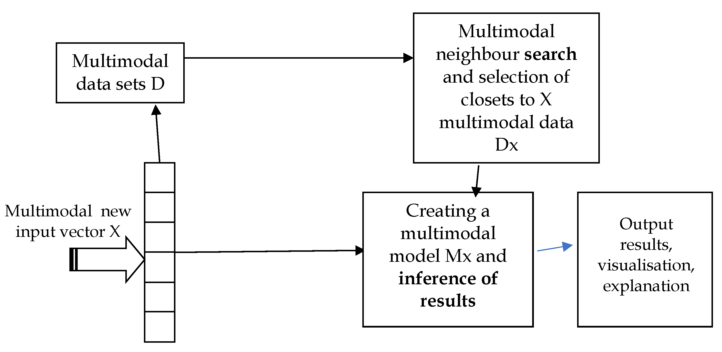
Figure 2.
A flow of data and information processing in the SAIN computational framework
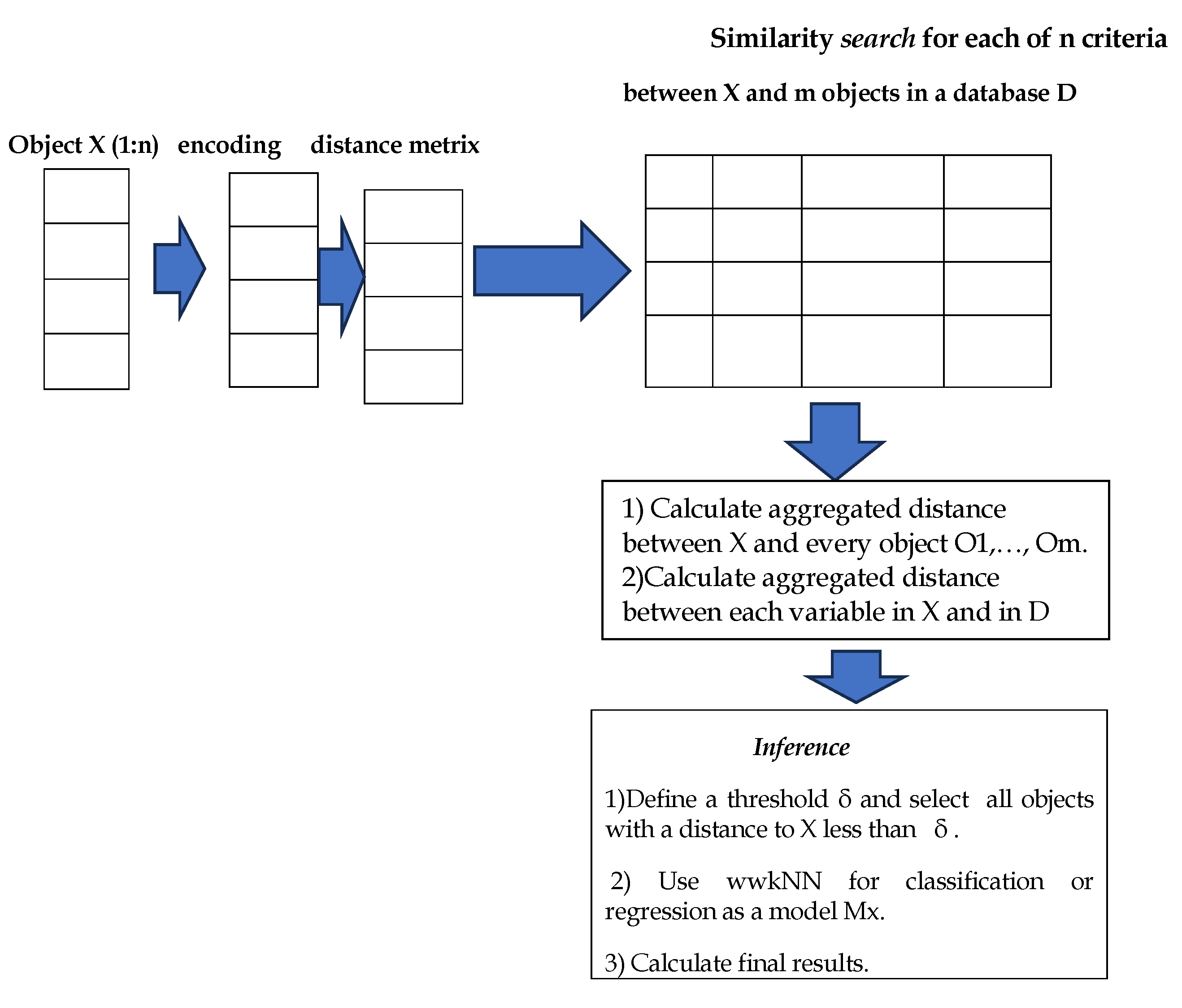
Figure 3.
Every time series can be represented as a 3-value vector through a spike encoding method over time [15]. If at a time t the times series is increasing in value, there will be a positive spike (1), if decreasing – negative spike (-1) and if no change – no spike (0) (left figure). Each element in this vector represents the change of the signal at a time. If necessary, the original signal can be recovered over time using this vector (right figure). The length of the vector is equal the time points measured.
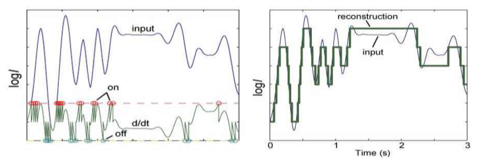
Figure 4.
EEG signals taken from EEG electrodes spatially distributed on the scalp are spatio- temporal signals (left figure). Each time series signal from an electrode is measured every 1 millisecond. The figure on the right shows the measurements of 14 EEG electrodes over time of 124 milliseconds. Each signal can be encoded into 124 element vector according to Figure 3, making altogether 14 such vectors to be processed in the SAIN framework.
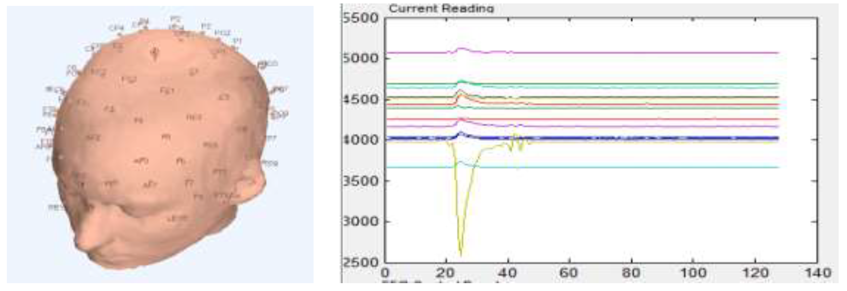
Figure 5.
ECG (Electro cardiogram) signals (a- nosy and b- filtered) can be encoded into binary vectors according to the spike encoding methods from Figure 3. Spike encoding is robust to noise, as any noise below a threshold would not cause the generation of a spike (either positive or negative) and the encoder will act as a filter. The length of this vector will be equal to the number of measurement time points. The vector data can be further processed in the SAIN framework.
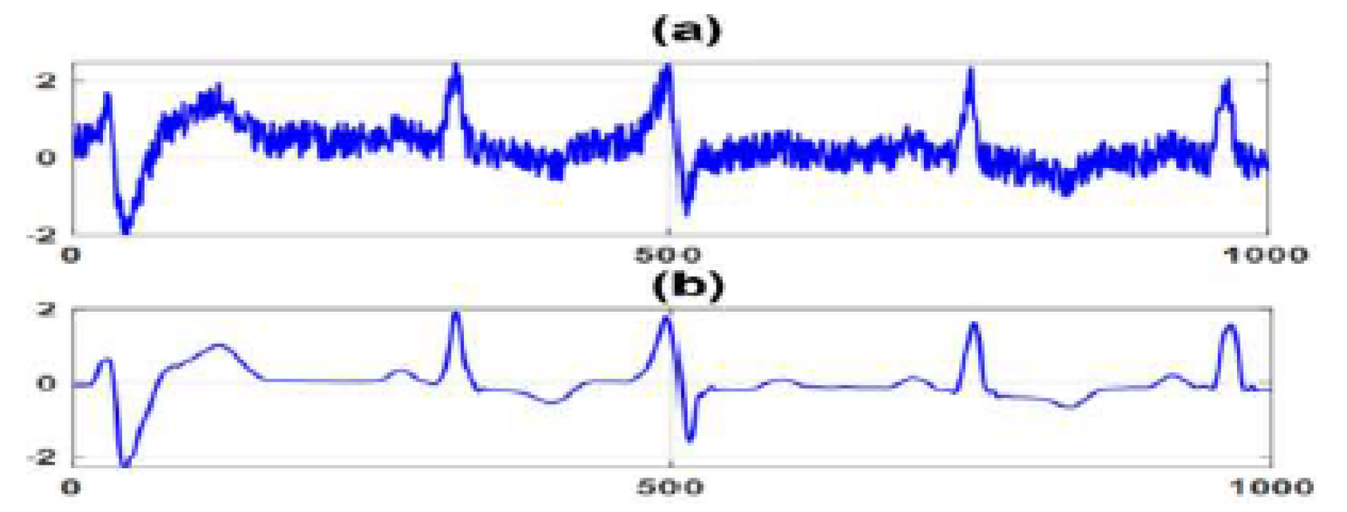
Figure 6.
Sample of the classification breakdown and the confusion matrix (class 2 would be utilised when we wish to have an uncertain class, but here we have classified based on probability ).
Figure 6.
Sample of the classification breakdown and the confusion matrix (class 2 would be utilised when we wish to have an uncertain class, but here we have classified based on probability ).
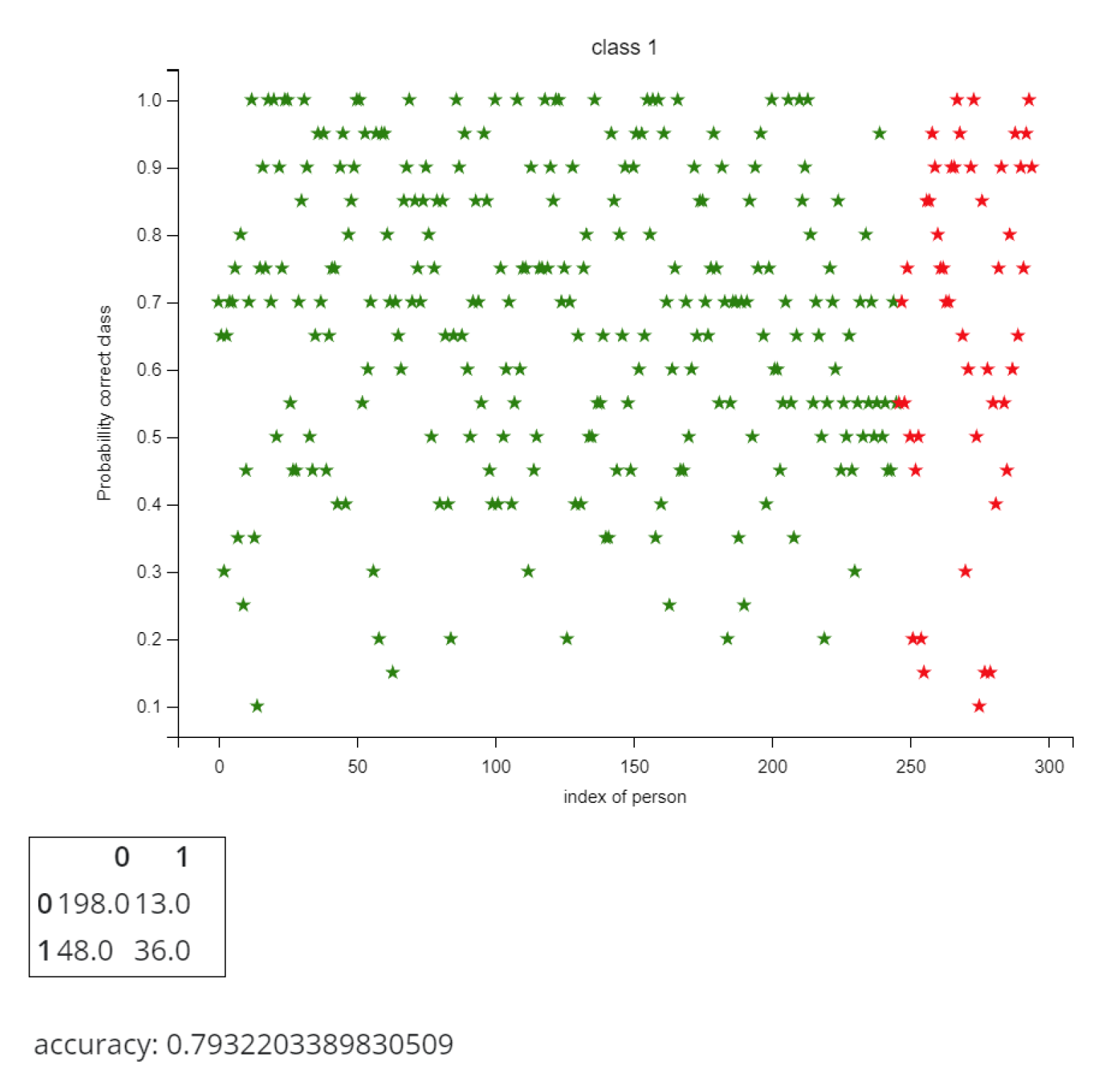
Table 2.
Labelled database.
| Objects/Criteria | ... | ... | Class label | ||||
| ... | ... | ||||||
| ⋮ | ⋮ | ⋮ | ... | ⋮ | ... | ⋮ | ⋮ |
| ... | ... | ||||||
| ⋮ | ⋮ | ⋮ | ... | ⋮ | ... | ⋮ | ⋮ |
| ... | ... |
Table 3.
Weights.
| Criteria weights | ... | ... | ||||
| w | ... | ... |
Table 4.
New unlabelled object.
| Object/Criteria | ... | ... | ||||
| x | ... | ... |
Table 6.
Example of labelled data.
| 68.2 | 0 | 6789 | small | red | 0,1,-1,-1,1,1,0,0, 1,-1 | 1,1,0 | 1 |
| 0,0,1 | |||||||
| 0,0,1 | |||||||
| 93 | 1 | 98000 | medium | yellow | 0,-1,-1,-1,-1,0,0, 1,-1,1 | 1,0,0 | 1 |
| 0,0,1 | |||||||
| 0,0,1 | |||||||
| 44.5 | 1 | 5600 | large | red | 0,1,-1,1,-1,1,0,0, 1,-1 | 1,1,0 | 1 |
| 1,0,1 | |||||||
| 1,1,1 | |||||||
| 56.8 | 0 | 89 | small | white | 1,-1,-1,-1,-1,1,0,0, 1,-1 | 1,1,0 | 1 |
| 0,1,1 | |||||||
| 1,0,1 | |||||||
| 26.3 | 0 | 9456 | large | black | 1,-1,-1,-1,0,1,0,0, 1,-1 | 1,1,0 | 2 |
| 1,1,1 | |||||||
| 1,0,1 | |||||||
| 81.5 | 1 | 78955 | medium | red | 0, 1,-1,1,-1,-1,0,0, 1,-1 | 1,1,0 | 2 |
| 0,0,1 | |||||||
| 1,1,1 | |||||||
| 56.7 | 1 | 68900 | small | black | 1,- 1,-1,1,-1,1,0,0, 1,1 | 1,1,1 | 2 |
| 0,0,1 | |||||||
| 1,1,1 | |||||||
| 20 | 0 | 7833 | large | yellow | 1,1,-1,-1,1,1,0,-1, -1,1 | 1,0,0 | 2 |
| 0,0,1 | |||||||
| 1,1,1 | |||||||
| 20 | 0 | 7833 | ∞ | yellow | 1,1,-1,-1,1,1,0,-1, -1,1 | 1,0,0 | 2 |
| 0,0,1 | |||||||
| 1,1,1 |
Table 7.
Example of new unlabelled object.
| 48.5 | 1 | 45679 | large | red | 1, 0, 0, -1, 1, -1, 1, 0, 0, 1 | 1,1,0 |
| 0,0,1 | ||||||
| 1,0,1 |
Table 8.
Coded labelled data.
| 68.2 | 0 | 6789 | 0 | FF0000 | 0122110012 | 110001001 | 1 | |
| 111111110000000000000000 | ||||||||
| 93 | 0 | 98000 | 1 | FFFF00 | 0222200121 | 110001001 | 1 | |
| 111111111111111100000000 | ||||||||
| 44.5 | 1 | 5600 | 2 | FF0000 | 0121210012 | 110101111 | 1 | |
| 111111110000000000000000 | ||||||||
| 56.8 | 0 | 89 | 0 | FFFFFF | 1222210012 | 110011101 | 1 | |
| 111111111111111111111111 | ||||||||
| 26.3 | 0 | 9456 | 2 | 000000 | 1222010012 | 110111101 | 2 | |
| 000000000000000000000000 | ||||||||
| 81.5 | 1 | 78955 | 1 | FF0000 | 0121220012 | 110001111 | 2 | |
| 111111110000000000000000 | ||||||||
| 56.7 | 1 | 68900 | 0 | 000000 | 1221210011 | 111001111 | 2 | |
| 000000000000000000000000 | ||||||||
| 20 | 0 | 7833 | 2 | FFFF00 | 1122110221 | 100001111 | 2 | |
| 111111111111111100000000 | ||||||||
| 20 | 0 | 7833 | ∞ | FFFF00 | 1122110221 | 100001111 | 2 | |
| 111111111111111100000000 |
Table 9.
New unlabelled object coded.
| x | 48.5 | 1 | 45679 | 2 | FF0000 | 1002121001 | 110001101 |
| 111111110000000000000000 |
Table 10.
Coded labelled normalised data.
| 0.682 | 0 | 0.06789 | 0 | 0.2 | 0.0122110012 | 0.110001001 | |
| 0.93 | 1 | 0.98 | 0.5 | 0.6 | 0.0222200121 | 0.100001001 | |
| 0.445 | 1 | 0.056 | 1 | 0.2 | 0.0121210012 | 0.110101111 | |
| 0.568 | 0 | 0.00089 | 0 | 1 | 0.1222210012 | 0.110011101 | |
| 0.263 | 0 | 0.09456 | 1 | 0 | 0.1222010012 | 0.110111101 | |
| 0.815 | 1 | 0.78955 | 0.5 | 0.2 | 0.0121220012 | 0.110001111 | |
| 0.567 | 1 | 0.689 | 0 | 0 | 0.1221210011 | 0.111001111 | |
| 0.2 | 0 | 0.07833 | 1 | 0.6 | 0.1122110221 | 0.100001111 | |
| 0.2 | 0 | 0.07833 | ∞ | 0.6 | 0.1122110221 | 0.100001111 |
Table 11.
New unlabelled object coded normalised.
| x | 0.485 | 1 | 0.45679 | 1 | 0.2 | 0.1002121001 | 0.110001101 |
Table 17.
Survival database.
| Patients/Criteria | ... | ... | Units of time | ||||
| ... | ... | ||||||
| ⋮ | ⋮ | ⋮ | ... | ⋮ | ... | ⋮ | ⋮ |
| ... | ... | ||||||
| ⋮ | ⋮ | ⋮ | ... | ⋮ | ... | ⋮ | ⋮ |
| ... | ... |
Table 18.
New patient record.
| Patient/Criteria | ... | ... | ||||
| p | ... | ... |
Table 21.
Distances between all patients and the new patient.
| Distance d | ||||||||
| 0.1970 | 1 | 0.388900 | 1.0 | 0.0 | 0.08800109890 | 0.000000100 | 2.67390119890 | |
| 0.4450 | 0 | 0.523210 | 0.5 | 0.4 | 0.07799208800 | 0.010000100 | 1.95620218800 | |
| 0.0400 | 0 | 0.400790 | 0.0 | 0.0 | 0.08809109890 | 0.000100010 | 0.52898110890 | |
| 0.0830 | 1 | 0.455900 | 1.0 | 0.8 | 0.02200890110 | 0.000010000 | 3.36091890110 | |
| 0.2220 | 1 | 0.362230 | 0.0 | 0.2 | 0.02198890110 | 0.000110000 | 1.80632890110 | |
| 0.3300 | 0 | 0.332760 | 0.5 | 0.0 | 0.08809009890 | 0.000000010 | 1.25085010890 | |
| 0.0820 | 0 | 0.232210 | 1.0 | 0.2 | 0.02190890100 | 0.001000010 | 1.53711891100 | |
| 0.2850 | 1 | 0.378460 | 0.0 | 0.4 | 0.01199892200 | 0.009999990 | 2.08545891200 | |
| 0.2850 | 1 | 0.378460 | 1.0 | 0.4 | 0.01199892200 | 0.009999990 | 3.08545891200 |
Table 22.
The 14 variables used in the heart disease diagnosis case.
| Name | Data type | Definition |
| age | integer | age in years |
| sex | binary | sex |
| cp | {1,2,3,4} | chest pain type |
| trestbps | integer | resting blood pressure |
| chol | integer | serum cholesterol in mg/dl |
| fbs | binary | fasting blood sugar > 120 mg/d |
| restecg | {0,1,2} | resting electrocardiographic results |
| thalach | I integer | maximum heart rate achieved |
| exang | binary | exercise-induced angina |
| oldpeak | float | ST depression induced by exercise relative to rest |
| slope | {1,2,3} | the slope of the peak exercise ST segment |
| ca | {0,1,2,3,} | number of major vessels colored by flourosopy |
| thal | {3,6,7} | heart status |
| num | {0,1,2,3,4} | diagnosis of heart disease |
Disclaimer/Publisher’s Note: The statements, opinions and data contained in all publications are solely those of the individual author(s) and contributor(s) and not of MDPI and/or the editor(s). MDPI and/or the editor(s) disclaim responsibility for any injury to people or property resulting from any ideas, methods, instructions or products referred to in the content. |
© 2025 by the authors. Licensee MDPI, Basel, Switzerland. This article is an open access article distributed under the terms and conditions of the Creative Commons Attribution (CC BY) license (http://creativecommons.org/licenses/by/4.0/).
Copyright: This open access article is published under a Creative Commons CC BY 4.0 license, which permit the free download, distribution, and reuse, provided that the author and preprint are cited in any reuse.


