
Submitted:
30 June 2025
Posted:
01 July 2025
You are already at the latest version
Abstract
This paper presents the development of a WebGIS tool for simulating wildfire spread and the associated smoke cloud dispersion, incorporating the wind field simulation—derived from point-based observational data—that influences both processes. The developed tool incorporates the following three physical models: HDWind for wind field simulation, PhyFire for wildfire spread, and PhyNX for smoke dispersion. It also integrates the necessary Geospatial Data Abstraction Library (GDAL) and Python scripts for preprocessing cartographic data and visualizing the simulation results—including wind fields, burned and burning areas, fire statistics, and smoke dispersion—at different time steps, with smoke dispersion additionally represented across multiple vertical levels. The WebGIS interface allows non-experts users to easily run simulations by defining the simulation area, ignition points, meteorological conditions, and firebreaks, as well as by configuring the parameters of the physical models involved. This tool aims to provide an accessible and user-friendly platform for wildfire simulation to aid in prevention and preparedness decisions. Finally, an example of how to use the interface is also presented.
Keywords:
WebGIS
; Wildfire simulation
; Smoke dispersion
; Wind field modeling
; Coupled physical models
; Geospatial data integration
; Environmental decision support systems
1. Introduction
Wildfires have become a growing global crisis, causing problems in ecosystems and human activities [1]. Over the last decade, the burned area, the fire season length and the fire severity have increased in multiple regions [2]. According to the Food and Agriculture Organization of the United Nations [3], wildfires burn around 340 million to 370 million hectares of land worldwide each year. In addition to their destructive impact, wildfires are a significant source of greenhouse gas emissions, affecting air quality even thousands of kilometers away [4]. Between 2000 and 2020, global wildfires released around 7.32 billion tons of CO2 annually, making up of the carbon dioxide produced by burning fossil fuels [5].
Understanding and forecasting the complex processes of wildfire spread and smoke plume dispersion are essential for forest fire managers, particularly in making prevention and preparedness decisions [6,7,8]. In both cases, accurate simulations rely on numerous variables, including orography, burned area, burning areas, fuel consumed, heat release rate, smoke plume [9], rate of spread (ROS), among others. However, wind has a higher-order impact on the spread and dispersion of both wildfire and smoke [10,11]. The use of wildfire spread and smoke dispersion models have been used for many years [12,13], but the recent technological development has increased their efficiency and applicability [14].
Multiple modeling of wildfire spread and smoke plume dispersion have been applied [15,16]. From empirical models for rapid post-wildfire assessments where information is collected, such as PROPAGATOR that is based on a Cellular Automata (CA) approach [17]; or quasi-empirical models such as FlamMap [18] and Prometheus [19]. To complex physical models incorporate some aspects of the combustion process and need an unlimited computing power, such as FIRETEC that uses computational fluid dynamics (CFD) models to predict fire spread in forest fires [20]; or quasi-physical models such as WRF-SFIRE [21] and MesoNH-ForeFire [22].
Visualization technologies have created significant opportunities for developing tools that offer easy access to information, are user-friendly and require lower computational resources [23]. These technologies are applied in various domains, including the simulation of wildfire spread and smoke plume dispersion, as understanding wildfires involves not only detecting their presence but also determining their location [24] and supporting decision-making processes. Geographic Information Systems (GIS) are among the most widely used technologies, primarily due to the spatial nature of wildfire-related data—such as forests, roads, settlements, and agricultural areas—which are essential for modeling wildfire spread and smoke plume dispersion [25,26]. For example, the system suggested by Bonazountas et al. [27] represents a desktop GIS solution that employs a unified user interface to create a comprehensive computer system. This system integrates fuel maps, socio-economic risk assessment, and probabilistic models to support forest fire prevention, planning, and management.
However, the Internet has rapidly transformed how geographic information is shared and distributed. The swift and widespread advancement of Internet technologies has established it as a key platform for accessing data, transmitting information, and leveraging GIS analysis tools [26]. The integration of Geographic Information Systems (GIS) and web technologies, known as WebGIS, allows the development of highly accurate and fast-executing models [28]. An example is the case of Gumusay and Sahin [26], who developed a web viewer for spatial datasets from various sources, or Kalabokidis et al. [29], who designed a platform that supports early fire warning, fire planning, fire control, and firefighting coordination by providing online access to critical wildfire management information.
A tool to simulate wildfire spread, wind dynamics, and smoke dispersion, has been developed, designed to be accessible and easy to use for non-expert users. The tool integrates, within a WebGIS environment that enables such accessibility, a core composed of three physical models: HDWind, for wind dynamics; PhyFire, for fire spread; and PhyNX, for smoke dispersion. These models are solved using efficient numerical and computational methods based on the finite element method, implemented in C++, using the custom finite element library, Neptuno++ [30]. Previous attempts to facilitate the use of these models by non-expert users included the development of an ArcGIS Add-in [31] and a web interface based on ArcGIS Server [32]. However, in both cases, the preprocessing of input data was not optimized. This limitation has been addressed in the current implementation, which leverages the functionalities provided by the Geospatial Data Abstraction Library (GDAL) [33] for efficient data preprocessing. Additionally, Python scripts are employed for the postprocessing of the simulation results. This modular design ensures the simulation coupled models are easily adapted to different GIS and has facilitated its integration into the WebGIS platform presented here.
This paper is structured as follows. Section 2 provides an overview of the Back-End and Front-End components that support the integration of wildfire simulation tools within the WebGIS platform. Section 3 presents a representative use case to demonstrate how the WebGIS can be used in practice. Finally, the paper concludes by summarizing the main findings and outlining directions for future research.
2. Materials and Methods
In this section, we discuss the integration of a suite of numerical simulation tools for wildfire-related phenomena within a WebGIS platform. The three models—designed to simulate wind fields, wildfire propagation, and smoke plume dispersion—have been developed by the Numerical Simulation and Scientific Computing Research Group (SINUMCC) at the University of Salamanca. The wind model provides localized wind field data, which are essential for accurately modeling fire behavior and smoke transport. Adapting these models to an operational WebGIS environment required the development of additional tools to ensure usability for non-expert users, including those without prior experience in numerical methods or wildfire simulation modeling.
Section 2.1 outlines the general hierarchy and interrelation of the tools, while Section 2.2 and Section 2.3 provide detailed descriptions of the Back-End and Front-End integrator modules, respectively.
2.1. WebGIS Architecture Overview
The architecture of the WebGIS presented in this work follows the typical client-server design of similar web-based applications, as depicted in Figure 1.
The Front-End application, which is executed in the web browser of the final user (client machine), features a graphic interface that allows the users to manage their simulations, along with a cartographic viewer equipped with the required interactive controls to perform the operations of preparing the geographical inputs and the parameter configuration of new wildfire simulations (configuration stage), as well as to explore and assess the results of already performed simulations (visualization stage). Further insights into the use of the Front-End implementation can be found in Section 3.
On the server side, the Back-End is made up of several services that are in turn configured to work together to offer a complete user experience. These services include a general governing service (Section 2.2.1), a database system (Section 2.2.2) for the management of both user-specific data and simulations, as well as information related to the internal geographical data sources required to perform simulations in different areas, a map server (Section 2.2.3), and the SINUMCC Simulation Toolset (Section 2.2.4). A detailed explanation of the Back-End internal structure can be found in Section 2.2.
2.2. Back-End Modules
2.2.1. Back-End Governing SINUMCC Web Service
The SINUMCC Web Service is a multi-component application that is responsible for coordinating all the Back-End operations, while at the same time also in charge of performing the communication tasks with the Front-End clients. Therefore, it plays several key roles within the application’s operational flow: (i) Firstly, it listens for incoming requests from the Front-End running on the client side, thus serving as the unique communication channel (apart from the internal maps server) between the client and the server; (ii) It also manages the user database, handling all related operations, such as logging-in validations, listing the user’s simulations and reviewing their configurations, etc.; (iii) In addition, it oversees the management of workspaces, which are the directories where input and output data for each simulation are stored. This includes creating the workspaces and generating the necessary configuration files for the SINUMCC Simulation Toolset; (iv) Finally, the service is responsible for launching and monitoring simulations once the execution command is issued.
The communications module is set to network in two scopes, a local one and a public one. The first scope is set to listen to the worldwide network and is intended to receive the calls from the Front-End application running in the web browsers of the clients. This listening service exposes an HTTP REST interface that handles POST requests to various endpoints (URLs), allowing clients to perform predefined operations by sending request-specific parameters in the body, typically as JSON data. Beyond the typical user session-specific actions in web-based applications, a list of endpoint requests includes listing of the user’s simulations, retrieving specific simulation configuration and progress status, obtaining cartographic representation of results from successful simulations, configuring and creating new simulations, and deleting existing simulations.
The second scope is restricted to a private network and is designed to allow communication between the SINUMCC Web Service and the host of the SINUMCC Simulation Toolset. Here, the SINUMCC Web Service dispatches execution commands to such host in order to start simulations within specific workspaces that would have been created previously. At the same time, simulation progress and status updates will be reported by each of the simulation instances running in above mentioned host via HTTP requests through this private network scope to another HTTP listening service.
Workspace management is one of the key tasks of the SINUMCC Web Service component in the Back-End. Here, it is important to define what a Workspace is in the context of the WebGIS, and what its contents are. Essentially, Workspaces are folders set to store all the input files that are needed to run a simulation within the SINUMCC Simulation Toolset, but also to store the results and log files. These folders are named using the UUID that is assigned to each simulation on-the-fly, and are stored on a shared network drive to which also the host of SINUMCC Simulation Toolset has read and write access. The initial contents of a Workspace prior to the start of a simulation include: (i) a simulation configuration file, which includes the paths for the input files and reference geospatial databases, the simulation bounding box, the model execution settings, and the instructions to perform the progress updates (i.e. the endpoint URL and the simulation ID to make the proper POST requests); (ii) a model parameters file as specified in Table 1; (iii) a meteorological information input file; (iv) a fire ignition point input file; (iv) optionally, other input files such as a firebreaks file. Further details on the input files required by the simulation models can be found in Section 2.2.4. A Workspace is created once a logged-in client requests the creation of a new simulation with a set of parameters.
2.2.2. Database
The implemented WebGIS employs a single non-relational database using the MongoDB engine. Here, we only do a simple description of the structure of such a database and its tables.
A users table includes the login and contact information of each user.
Simulation data is structured in a simulations table, which stores basic data such as each simulation UUID, title description, progress and owner in separate fields, while general simulation configuration settings are encoded as JSON and stored in a single string field.
Finally, another table named simulationsources is in charge of keeping track of the internal geographic information sources available for each region or pilot.
Its structure contains a field for a bounding box that represents the simulation area where there are data available, another field storing the path of the geospatial database, its reference system, and its type; i.e., whether it is a digital elevation model (DEM), a firebreaks database, or a vegetation type map. This table is used by the SINUMCC Web Service module in order to establish the origin of the data sources to generate the cartographic input files that will be used in the simulations.
2.2.3. Internal Map Server
The map server is the component responsible for enhancing the user experience by enabling the exploration of internal cartographic data available for each region. It has to be noted that these maps can be stored either in raster or vector format, but are always provided in a raster format for visualization inside the browser-based GIS viewer as it will be later explained in Section 2.3. Specifically, three key maps required for fire and smoke simulation are provided through the Web Map Service (WMS) protocol: a DEM, a fuel type map classified according to the National Forest Fire Laboratory (NFFL) system [34], and a fuel presence map that identifies areas devoid of vegetation, which may function as natural firebreaks and, therefore, fire cannot propagate.
2.2.4. SINUMCC Simulation Toolset
The SINUMCC Simulation Toolset provides wildfire simulation capabilities through a modular architecture. It comprises two main components: the Launcher, a collection of Python scripts responsible for managing simulation execution as well as preprocessing and postprocessing tasks; and the Core, which includes the model binaries—HDWind for wind field simulation, PhyFire for fire spread modeling, and PhyNX for smoke dispersion—alongside the finite element library Neptuno++.
-
Launcher The Launcher is composed of a collection of Python scripts that provides added functionality aimed to ease the treatment of geospatial information and the integration of the Core tools in a GIS. Its main task is handling a sequence of operations that are divided into: (i) preprocessing tasks, (ii) simulation execution, and (iii) postprocessing tasks. Throughout these steps, the Launcher also gathers the progress of each of them, and reports to the main SINUMCC Web Service in the Back-End, allowing the whole tracking of the simulation from the Front-End.The devised preprocessing tasks involve cropping and reprojecting the information found in the global/regional internal geospatial databases used as the three cartographic input data–the DEM, the fuel type map and the fuel presence map–, as outlined at the end of this section. These operations are done according to the instructions set in the main configuration file, including the simulation bounding box, the UTM reference system chosen for the simulation in the specific geographical region, the spatial resolution, and the path to the original internal datasets. This way, all the input files will be georeferenced using the same projection system and resolution, thus achieving consistency between the different raster inputs is achieved in a single step. Furthermore, any raster or vector file formats can be used as global/regional input datasets (except for the DEM, where only raster is allowed) as long as they are supported by the GDAL library. These tasks are performed by several Python modules that are called by the Launcher, and make an intensive use of the GDAL library bindings.The Python script allows to process more efficiently the set of GIS vector layers of simulation results. In the simulation stage, the Launcher calls the Core binary to perform the numerical calculations. In the meantime, the output messages that reveal the stage along the different steps that the simulation undergoes, are reported through POST requests to the main governing SINUMCC Web Service in the Back-End. Finally, once the simulation Core finishes the simulation, the Launcher triggers the postprocessing stage. In order to simplify the access to the simulation results by the end-user, a postprocessing task is set to gather all the individual files for each graphical output time step into a single Spatialite database in which each element (features representing the burning area, the burned area, the wind field, smoke concentration, etc.) is labeled with its respective time tag. This allows the Front-End specifications for the visualization of results to be fulfilled as well as facilitating the downloading of simulation results in a single file.
Detailed descriptions of the simulation models are beyond the scope of this work; instead, their roles are briefly outlined, with references to original publications detailing their formulation and validation.
Furthermore, an understanding of how the models are coupled is required prior to their description (see Figure 2). The wind field at the surface level, produced by the HDWind model, serves as input for the PhyFire wildfire propagation model. Simultaneously, the complete 3D wind field is employed by the PhyNX model to simulate atmospheric smoke dispersion. The lower boundary condition for PhyNX is defined by the quantity of solid fuel consumed, which is calculated by PhyFire based on an emission factor that must be calibrated to estimate smoke emissions accurately. The tool also supports the decoupled use of the models, in the sense that it is possible to simulate wildfire spread alone—either under uniform wind conditions or using wind fields computed by the HDWind model—without performing the smoke dispersion calculation when it is not required. Conversely, joint fire and smoke simulations can also be conducted under either uniform wind conditions or wind fields generated by the HDWind model, depending on data availability. This flexibility significantly reduces computational cost, as smoke dispersion involves a fully 3D simulation, which is substantially more demanding in terms of resources.
-
HDWind: High-definition wind field modelThe HDWind model is developed to simulate the wind field within an atmospheric layer situated just above the surface S, where wildfire propagation occurs. This layer is influenced by surface temperature and local topography, whereas above it, these effects are considered negligible. As a result, the 3D domain in which the Navier–Stokes equations are formulated is assumed to have a substantially smaller vertical extent compared to its horizontal dimensions. This assumption allows for an asymptotic approximation of the Navier–Stokes equations, inspired by the principles underlying shallow water models. The model aims to generate a detailed 3D wind field over the study area by solving only 2D linear equations. To achieve this, we assume a linear decrease in air temperature with height, and neglect the nonlinear terms. This approach enables efficient coupling with the 2D fire spread model PhyFire, thereby minimizing the computational cost of the HDWind–PhyFire integration. The theoretical framework for the asymptotic simplification of the Navier–Stokes equations used to derive this model is detailed in Asensio Sevilla et al. [35] and Asensio et al. [36].In the proposed model, the 3D wind field is derived from the solution of a 2D potential problem, which is driven by the meteorological wind specified at the boundary of the domain. In practice, however, such boundary wind data are unavailable. Instead, wind speed and direction are typically measured at discrete points within the domain, such as meteorological stations. To incorporate these observations, the problem is reformulated so that the input data correspond to pointwise wind measurements rather than boundary conditions. This is accomplished by posing an optimal control problem, in which the boundary wind field acts as the control and is adjusted to best fit the available observational data. The computational strategy adopted to address this optimal control problem is presented in detail in Ferragut et al. [37].The HDWind model is a flexible and adaptable local-scale wind model. It is valuable not only for improving localized wind data relevant to wildfire spread but also for simulating various atmospheric processes, such as the dispersion of pollutants, wildfire smoke, and for estimating wind energy production [38].
-
PhyFire: Fire spread model PhyFire is a 2D simplified physical one-phase wildfire spread model incorporating certain 3D effects. It is based on the principles of energy and mass conservation, considering radiation and convection as the primary heat transfer mechanisms, while also accounting for heat loss in the vertical direction due to natural convection. The single phase represents the solid phase, while the gaseous phase is accounted for through a parameter influencing the convective term, as well as the flame temperature and height in the radiation term, both of which are determined using dedicated submodels. The model also incorporates the effects of fuel continuity and type, along with fuel moisture content, the latter being represented by a multi-valued operator in the enthalpy. Additionally, it considers flame tilt caused by wind or terrain slope. An optional feature allows for the integration of stochastic phenomena such as fire-spotting. The associated simplified system of partial differential equations (PDEs) yields, at each instant and for every point on the surface where fire spread is modeled, two dimensionless variables: the dimensionless temperature of the solid fuel (u) and the mass fraction of solid fuel (c), with the third variable in the system being the dimensionless enthalpy (e).The first version of this model accounted for local radiation using a Rosseland approximation and included a reactive term based on Arrhenius’ law (see Asensio and Ferragut [39]). Two major simultaneous improvements were introduced in Ferragut et al. [40] and Ferragut et al. [41]: first, non-local radiation, which allowed the incorporation of 3D effects while maintaining the model’s 2D simplicity ; and second, a multi-valued operator in the enthalpy to model the effect of fuel moisture content (FMC) on fire spread. This novel approach to incorporating FMC effects aligns with the exponential decay in the ROS induced by this factor (see Asensio et al. [42]). The current version of the model integrates the aforementioned submodels for flame temperature and height, as well as the ability to simulate certain random phenomena. Full details on the evolution of the PhyFire model, as well as its current version, can be found in Asensio et al. [43]. The PDEs defining the model are complemented by the appropriate boundary and initial conditions, which establish the initial state of the fuel and the ignition point. The problem is solved using efficient numerical methods based on the finite element method (FEM). The code is also adapted for parallel computing using OpenMP, significantly reducing simulation time. The total computation time depends on factors such as the simulation domain size, time step, and spatial resolution. Notably, simulating one hour of fire spread under moderate conditions with intermediate resolution on a standard computer takes less than two minutes.
-
PhyNX: Atmospheric dispersion model PhyNX is a multilayer, non-reactive Eulerian model designed for urban-scale air quality assessments. It simulates convection and diffusion processes, is grounded in the mass conservation equation, and is specifically adapted to model the dispersion of smoke plumes originating from wildfires. The model operates within the atmospheric layer above the fire-affected surface S and is coupled with the wildfire spread model PhyFire through a boundary condition defined at the surface S. Smoke emissions from the simulated fire are calculated as a function of the amount of fuel consumed, modulated by an emission factor that depends on the fuel type. The model also assumes that smoke losses occur only at the lateral boundary, but not at the upper boundary, and that there is no deposition on the surface S.Accurate and stable numerical schemes are essential for solving air dispersion models. To address this, an Adaptive Finite Element Method incorporating characteristics in the horizontal plane, combined with Finite Differences in the vertical direction, has been implemented. This was achieved through operator splitting techniques and a parallelized algorithm. Operator splitting is a well-established strategy in the numerical solution of air dispersion problems, as it facilitates the decomposition of complex systems into more manageable subproblems. Our approach enables the horizontal convective and diffusive terms to be solved concurrently for each horizontal layer, allowing for increased resolution by refining the number of layers without a proportional rise in computational cost. The vertical discretization relies on the wind field provided by the HDWind model, which supplies wind data for each atmospheric layer. As a result, the method achieves high accuracy while preserving real-time or faster-than-real-time performance. For further details on the numerical scheme, its parallel implementation, and the coupling between the atmospheric dispersion model PhyNX and the wind field model HDWind, see Ferragut et al. [44].
- Neptuno++: Finite Element library Neptuno++ is an adaptive finite element toolbox mainly developed by L. Ferragut at SINUMCC [30] and implemented in C++. It uses 4TRivara’s refinement and error control, enabling effective solutions for both stationary and time-dependent problems. This library has been utilized to validate convergence theories in Adaptive Finite Element Methods and has been applied for the numerical simulation of several environmental problems. The current version of this library provides functionalities for handling geospatial data.
In the context of this work, it is essential to provide a more detailed explanation of the model components that serve as a link to the WebGIS, specifically the input and output data, as well as the parameters that can be modified through this interface. Figure 2 also provides an overview of the input and output data for each model, while Table 1 lists the parameters associated with each model, distinguishing those that also depend on the fuel type. All these parameters are configurable through the WebGIS platform.
Cartographic input data required by the HDWind model include the DEM and the fuel type map of the simulation area. Furthermore, the PhyFire model additionally requires fuel presence map. Moreover, the fuel presence map can be modified through the platform to introduce potential changes in fuel distribution—such as the position and width of new firebreaks—and it defines the initial value of the dimensionless solid fuel variable in the model. Similarly, the initial value of the dimensionless solid fuel temperature, which is defined by the location of the ignition source(s), is set through the platform. The fuel types determines fire behavior for each fuel category through a set of parameters in the fire spread model, whose values depend on the fuel type and are listed in Table 1. It also determines the surface roughness coefficient, which influences wind calculations in the HDWind model.
The models also rely on meteorological inputs, including ambient temperature, relative humidity, and wind direction and intensity. All of these data can be updated hourly through the platform. Wind-related information, in particular, requires additional explanation. Two options are available for wind data. The first assumes a uniform wind across the simulation area, which can be updated hourly during the simulation. This approach uses only the fire spread model, without coupling it with the HDWind model. The second option integrates the HDWind and fire spread models and requires georeferenced wind intensity and direction data at specific locations. These data are used by the HDWind model to compute a 3D wind field over the simulation area. As previously mentioned, the wind field in the lower layer is used as input for the fire spread model, while the remaining layers are used for the smoke dispersion model.
The PhyFire model provides, at each of the graphical output time and at each point on the surface where fire spread is simulated, two dimensionless variables: the dimensionless temperature of the solid fuel and the mass fraction of solid fuel. These variables are processed through Boolean operations involving the initial fuel temperature and fuel load to determine both the areas that have already burned and those that are actively burning. As a result, the model output is not limited to a line representing the fire front position, but also includes its depth. Additionally, the model generates key statistics for each of the graphical output time, including the total burned area (in hectares), the actively burning area (in hectares), the distance from the ignition point to the most advanced point of the fire front, and the ROS at that point.
The PhyNX model provides the smoke concentration at each output time step and at every point within each of the air layers used in the vertical discretizations; both the total height of the 3D domain of the air layer and the individual layers for which the smoke output is generated are easily selected through the WebGIS interface. Initially, the model is designed to simulate the dispersion of the smoke plume without distinguishing its components. However, it can be easily adapted to simulate the behavior of the main components of wildfire smoke, provided that the emission factors for each of these components are known.
As previously explained, the physical models are solved within a defined domain that includes: (i) the simulation area, understood as the rectangular region on the surface where the wildfire occurs; (ii) the simulation time interval, which must be shorter than the time required for the fire to reach the boundary of the simulation area, thereby ensuring the validity of homogeneous Dirichlet boundary conditions; and (iii) the height of the air layer over which smoke dispersion is computed. All of these settings can be easily configured through the WebGIS platform, as described in Section 3.
Several numerical parameters also need to be configured, including the horizontal element size of the 2D finite element mesh defined on the simulation area, and the number of vertical air layers in which wind field and smoke concentrations are computed and displayed. Additionally, while the time step used for the numerical integration is predefined, the user can select the output time interval for graphical results, which controls the frequency at which simulation data are saved and visualized.
In addition, each model includes a set of parameters with pre-calibrated default values, which the user can modify through the WebGIS interface. These parameters can be classified into two categories. On one hand, there are model-specific parameters—for instance, those associated to the optimal control problem of the HDWind model, or with the three heat transfer mechanisms considered by the PhyFire model (radiation, convection, and vertical natural convection), or the horizontal and vertical dispersion coefficients used in the PhyNX model. On the other hand, there are parameters whose values depend on the type of fuel. For example, the surface roughness parameter in the HDWind model, the emission coefficient in PhyNX, and up to eight fuel-related parameters in PhyFire, which are listed in Table 1. Detailed explanations of these pre-calibrated parameter values can be found in Prieto et al. [45], Asensio-Sevilla et al. [46] and Asensio et al. [42]. While these values are based on preliminary calibration efforts, further refinement and validation remain ongoing.
2.3. Front-End
The Front-End application consists of a website comprising three modules: a login page, a user dashboard, and a GIS component that functions as both a simulation results viewer and a simulation configuration interface. The Front-End is written using the React.js framework, while the GIS viewer is running over the javascript OpenLayers library.
Both the login and dashboard components feature a straightforward design and do not incorporate technically innovative or noteworthy elements, relying instead on conventional approaches commonly employed in contemporary web applications.
Certain aspects of the GIS viewer warrant further examination. The map viewer provides the possibility to use several publicly available map base sources such as Bing, Google, OpenStreetMap (OSM), or ArcGIS. It also provides a layer manager that classifies the data sources in two groups: (i) input layers; and (ii) reference cartography. This latter group includes the DEM, the fuel types, and the fuel presence layers served through the WMS protocol by the internal cartography map server, but also other DEM data sources as Copernicus, the European-level fuel type cartography from EFFIS, or country-specific orthophoto imaging. In the input layers, there is the simulation area, the initial ignition point, the wind reference point or stations, and the firebreaks or firefighter actions.
As it regards the input layers, these would be populated during the creation of a new simulation throughout the configuration stage, by using a multi-tab configuration panel, and a toolbar-type interface to access the available features, including the following tools: (i) an access to the general configuration tab in the configuration panel; (ii) a simulation area selection tool; (iii) an access to the meteorological input configuration tab; (iv) setting up the initial ignition point(s); (v) setting up firebreaks; (vi) setting up meteorological reference points or stations; and (vii) resetting the configuration.
Regarding the configuration panel, it holds all the input forms and controls to fully configure the simulation within the application capabilities. The tabs are the following: (i) Metadata, allowing to set a title, description and date of the start for the event; (ii) General options, which include the time span for the simulation, the frequency of saving results, the precision of the simulation, and whether the smoke simulation must be enabled or not; (iii) Meteorology, which allows to configure whether the simulation will be run with an uniform wind, or a wind computed through HDWind; (iv) Fuels, permitting to manipulation of the different parameters that govern the fire behavior of each of them; (v) and (vi) PhyFire and HDWind specific model parameters; and (vii) PhyNX specific model parameters if it was selected.
The visualization stage incorporates the same tools as the configuration stage. However, the intention of the configuration of panel and toolbar here is only to review the simulation configuration settings. Furthermore, the toolbar includes a log that allows viewing the output generated by the SINUMCC Simulation Toolset. Since the simulation results are time-tagged, along with a new group in the layers panel, another floating tool appears in the map viewer interface: a time slider and photogram controller. The simulation results available layers are: (i) wind field; (ii) burned area; (iii) burning area; (iv) simulation statistics providing some useful data such as the output time step in hours, the ROS in m/min, the extent (ha) of the burned and burning areas; and (v) smoke concentration, if PhyNX was selected. The activation of the layers, along with the selection of an instant with the time slider, activates a request to the SINUMCC Web Service to retrieve such cartographic information, that is in turn sent back to the client in GeoJSON format for visualization.
3. Results: WebGIS Usage
To illustrate the functionality of the proposed WebGIS platform, this section presents a representative use case detailing the complete workflow, including all available options for configuring and executing the three coupled models—HDWind, PhyFire, and PhyNX—for simulating wildfire spread and smoke plume dispersion within a GIS-based environment. This example also highlights the system’s capability to accurately predict fire behavior and smoke dynamics.
The workflow of how the simulation tool is used in WebGIS can be split into three main stages (Figure 3). In the first stage, the user selects the simulation configuration parameters from the Front-End. Next, the WebGIS Back-End consists of simulating as detailed in the Launcher description in Section 2.2.4. Finally, the third stage is visualizing the simulation results in the WebGIS Front-End. The different steps of each stage can be performed in different ways, with mouse events (M-number in Figure 3), pop-up windows (W-number in Figure 3) or toolbar (S-number in Figure 3).
1. Front-End: Configuration stage
The initial stage comprises eight sequential steps. The first five are mandatory for initiating the simulation process and are designed to be completed without requiring detailed knowledge of the underlying physical models. The final three steps offer advanced customization options and can be either left at default values or modified as needed—for instance, to add optional firebreaks, enable the fire-spotting feature, or adjust the values of model parameters listed in Table 1.
In the first step, the Configuration pop-up window is opened. Within this window, it is necessary to access the Metadata tab (W-I in Figure 3), where the date, title and description of the simulation event should be specified as shown in the left of Figure 4 and then saved. In the same window, access the Options tab (W-II in Figure 3) to select the simulation time interval (between 1 and 8 hours), the output time interval for graphical results (15, 30 or 60 minutes) and the spatial resolution (which is set by default to 7.5 meters but can be modified—through the WebGIS interface—to 5, 7.5, 10, 20, or 50 meters). In the presented use case, the Options settings are shown in the right of Figure 4.
The second step consists of selecting the simulation area with a maximum allowed area of using the mouse event (M-II in Figure 3). The selected area for this use case can be visualized through various map layers (see in Figure 5). These layers assist the users in identifying vegetation patterns, firebreaks, and anthropogenic elements for accurate configuration of wildfire simulations (M-I and S-I in Figure 3).
The third step involves an additional mouse interaction to identify the ignition sources
of the fire within the simulation area (M-III in Figure 3). The location of the fire ignition point is illustrated in the top left of Figure 6.
The next step is defining the meteorological data within the Meteorology tab of the Configuration pop-up window. The required inputs include wind intensity (Km/h), wind direction (North, Northeast, East, Southeast, South, Southwest, West, Northwest), height (meters), ambient temperature (°C) and relative humidity (%). Two modes of data entry are available. If the Punctual Wind Data option is selected (M-IV in Figure 3 and in the bottom left of Figure 6), the configuration process proceeds directly to the next stage. Alternatively, if the Uniform Data option is selected (M-IV in Figure 3 and in the top right of Figure 6), the corresponding meteorological values must be manually entered for each simulated hour (W-III in Figure 3 and in the top right of Figure 6). The configuration selected for this use case is the Punctual Wind Data option as shown in the bottom left of Figure 6, which involves the use of the HDWind wind model.
The fifth step is applicable only when Punctual Wind Data has been chosen. This step consists of marking one or more punctual meteorological with the mouse (M-V in Figure 3); in this use case, two ignition points have been set, as shown in the bottom left of Figure 6. The system automatically queries the NASA POWER database to retrieve meteorological data for this location (W-IV in Figure 3), but in this presented case, it is changed as shown in the bottom left of Figure 6.
Once the required data have been entered to run the simulation, the tool allows configuration of the final three steps of this stage. For advanced users, the system permits modification of the initial fuel data obtained in step three by enabling the drawing of new firebreaks during step six through direct mouse interaction (M-VI in Figure 3). Furthermore, the tool allows the selection of the width of the located firebreak in meters (W-V in Figure 3). In this use case, a firebreak is placed as shown in the bottom right of Figure 6 with a width of 10 meters.
The seventh and eighth steps allow modification of the parameter settings of the models listed in Table 1 according to their specific interests, making this simulation tool highly versatile. In the Configuration pop-up window, several tabs are available to access each type of parameter. The Fuels tab provides access to parameters dependent on the fuel type (W-IX in Figure 3 and in the top left of Figure 7); the PhyFire tab allows configuring the main parameters of this model, including the option to activate fire-spotting (W-VII in Figure 3 and in the bottom left of Figure 7); the HDWind tab provides access to the main parameters of the HDWind model (W-VI in Figure 3 and in the top right of Figure 7); and finally, if the smoke simulation option has been enabled in the configuration settings, an additional tab named PhyNX will appear, granting access to the main parameters of that model (W-VIII in Figure 3 and in the bottom right of Figure 7). In this presented case, all parameters must be left by default, with only the smoke simulation option activated and the parameter height of the air layer changed to 80,00 m (bottom right of Figure 7).
2. Back-End
The second stage involves launching the simulation based on all parameters and input data defined during the initial configuration stage. This process is initiated by clicking the circular run button located at the top right corner of the interface.
Once the run button is pressed, the system first verifies that all required steps in the configuration stage have been completed. If any configuration fields are highlighted in red, this indicates incomplete or incorrect input (M-VII in Figure 3), and the simulation will not proceed. Conversely, if all inputs are valid, the simulation is launched, where the workspace is prepared and the Launcher is called to execute all steps explained in Section 2.2.4.
3. Front-End: Visualization stage
Finally, the third stage is visualizing he simulation results (S-II in Figure 3). To see all results for each previously defined time step, the green play icon located on the time slider must be pressed.
For the simulation results available layers are: the wind field (top left in Figure 8), burned area (top right in Figure 8), burning area (top right in Figure 8), simulation statistics (top right in Figure 8). Furthermore, the simulation results available layer of the PhyNX model is the smoke, which is represented at different height levels (bottom left and bottom right in Figure 8).
It is also possible to view a 3D animated video of the simulation results of the PhyFire model which can be accessed by clicking on the button with the camera icon (W-X in Figure 3). This video provides a more realistic image of the results by projecting the fuel layers on the orthophoto of the simulation area.
With respect to the 3D simulation results, such as the smoke cloud and the wind field at different height levels, clicking the photo controller.
Once the three models are simulated and display results, the simulation log can be reviewed and data downloaded using the buttons of the W-XII and W-XI in Figure 3.
4. Discussion
This paper presents the development and implementation of an integrated WebGIS-based simulation tool that couples wind field modeling, wildfire spread, and smoke dispersion. The system incorporates three physical models—HDWind, PhyFire, and PhyNX—coupled through a modular and efficient computational architecture and supported by a user-oriented WebGIS interface. This integration enables the simulation of complex wildfire-related processes with a high level of realism, while maintaining accessibility for non-expert users.
This new version represents a significant technical improvement over previous implementations, such as those based on ArcGIS tools. A key innovation is the integration of the GDAL library for the automated preprocessing of geospatial data, which significantly enhances efficiency and interoperability. In addition, the modular design facilitates seamless coupling of the physical models and their execution within a unified WebGIS environment. These advancements contribute to greater computational performance, reduced user workload, and a more streamlined simulation workflow.
The tool allows for the configuration and execution of simulations with minimal technical knowledge, making it highly suitable for operational use in risk assessment, emergency planning, and decision-making processes. The incorporation of pre-calibrated model parameters, automated preprocessing and postprocessing, and interactive visualization features support a complete workflow from configuration to analysis of simulation outcomes.
Future research will focus on expanding the functionalities of the platform, including the integration of real-time meteorological data sources, enhanced 3D visualization tools, and the simulation of specific smoke constituents. Additionally, ongoing efforts are directed toward further model validation and sensitivity analyses to increase predictive accuracy and operational robustness.
Supplementary Materials
The following supporting information can be downloaded at the website of this paper posted on Preprints.org. A video demonstrating an example of how to use the WebGIS interface is provided as supplemental material and can be accessed via DOI: 10.6084/m9.figshare.29290628. This video illustrates the main functionalities and user interactions described in the manuscript.
Author Contributions
Conceptualization, M. Isabel Asensio; Data curation, José M. Iglesias and David Cifuentes-Jiménez; Formal analysis, M. Isabel Asensio; Funding acquisition, Diego González-Aguilera; Investigation, Saray Martínez-Lastras, José M. Iglesias and M. Isabel Asensio; Project administration, Diego González-Aguilera; Resources, José M. Iglesias and David Cifuentes-Jiménez; Software, David Cifuentes-Jiménez; Supervision, M. Isabel Asensio and Diego González-Aguilera; Validation, José M. Iglesias; Writing – original draft, Saray Martínez-Lastras; Writing – review & editing, José M. Iglesias and M. Isabel Asensio.
Funding
This work was supported by the European Union’s Horizon 2020 - Research and Innovation Framework Programme under Grant 101036926; and the Ministerio de Ciencia, Innovación y Universidades under Grant FPU21/00446.
Data Availability Statement
Data underlying this study can be provided by the corresponding author upon reasonable request, subject to institutional considerations.
Conflicts of Interest
The authors report there are no competing interests to declare.
Abbreviations
The following abbreviations are used in this manuscript:
| CA | Cellular Automata |
| CFD | Computational Fluid Dynamics |
| DEM | Digital Elevation Model |
| EFFIS | European Forest Fire Information System |
| FMC | Fuel Moisture Content |
| GDAL | Geospatial Data Abstraction Library |
| GIS | Geographic Information Systems |
| HDWind | High-definition wind field model |
| NFFL | National Forest Fire Laboratory |
| OSM | OpenStreetMap |
| PNOA | Spanish National Plan for Aerial Orthophotography |
| ROS | Rate of Spread |
| SINUMCC | Numerical Simulation and Scientific Computing Research Group |
| PhyFire | Physical Fire spread model |
| PhyNX | Atmospheric dispersion model |
| VHR | Very high resolution |
| WMS | Web Map Service |
References
- Crist, M.R. Rethinking the focus on forest fires in federal wildland fire management: Landscape patterns and trends of non-forest and forest burned area. Journal of Environmental Management 2023, 327, 116718. [Google Scholar] [CrossRef]
- Valero, M.; Rios, O.; Mata, C.; Pastor, E.; Planas, E. GIS-based integration of spatial and remote sensing data for wildfire monitoring. In Proceedings of the Earth Resources and Environmental Remote Sensing/GIS Applications IX; 2018. [Google Scholar]
- FAO. FAO launches updated guidelines to tackle extreme wildfires, 2024. Accessed: March 2025.
- Lee, K.H.; Kim, J.E.; Kim, Y.J.; Kim, J.; Von Hoyningen-Huene, W. Impact of the smoke aerosol from Russian forest fires on the atmospheric environment over Korea during May 2003. Atmospheric Environment 2005, 39, 85–99. [Google Scholar] [CrossRef]
- Liu, Z.; He, H.; Xu, W.; Liang, Y.; Zhu, J.; Wang, G.G.; Wei, W.; Wang, Z.; Han, Y. Impacts of forest fire carbon emission and mitigation strategies. Bulletin of Chinese Academy of Sciences 2023, 38, 1552–1560. [Google Scholar] [CrossRef]
- Yin, L.; Shaw, S.L.; Wang, D.; Carr, E.A.; Berry, M.W.; Gross, L.J.; Comiskey, E.J. A framework of integrating GIS and parallel computing for spatial control problems–a case study of wildfire control. International Journal of Geographical Information Science 2012, 26, 621–641. [Google Scholar] [CrossRef]
- Meng, Q.; Huai, Y.; You, J.; Nie, X. Visualization of 3D forest fire spread based on the coupling of multiple weather factors. Computers and Graphics 2023, 110, 58–68. [Google Scholar] [CrossRef]
- Prichard, S.; Larkin, N.S.; Ottmar, R.; French, N.H.F.; Baker, K.; Brown, T.; Clements, C.; Dickinson, M.; Hudak, A.; Kochanski, A.; et al. The Fire and Smoke Model Evaluation Experiment—A Plan for Integrated, Large Fire–Atmosphere Field Campaigns. Atmosphere 2019, 10, 66. [Google Scholar] [CrossRef] [PubMed]
- Shamsaei, K.; Juliano, T.W.; Roberts, M.; Ebrahimian, H.; Lareau, N.P.; Rowell, E.; Kosovic, B. The Role of Fuel Characteristics and Heat Release Formulations in Coupled Fire-Atmosphere Simulation. Fire 2023, 6, 264. [Google Scholar] [CrossRef]
- Filippi, J.B.; Bosseur, F.; Mari, C.; Lac, C.; Moigne, P.L.; Cuenot, B.; Veynante, D.; Cariolle, D.; Balbi, J.H. Coupled Atmosphere–Wildland Fire Modelling. Journal Advanves in Modelling Earth Systems 2009, 1, 9. [Google Scholar] [CrossRef]
- Kochanski, A.; Jenkins, M.A.; Sun, R.; Krueger, S.; Abedi, S.; Charney, J. The importance of low-level environmental vertical wind shear to wildfire propagation: Proof of concept. Journal of Geophysical Research: Atmospheres 2013, 118, 8238–8252. [Google Scholar] [CrossRef]
- Pastor, E. Mathematical models and calculation systems for the study of wildland fire behaviour. Progress in Energy and Combustion Science 2003, 29, 139–153. [Google Scholar] [CrossRef]
- Peacock, R.D.; Jones, W.W.; Bukowski, R.W. Verification of a model of fire and smoke transport. Fire Safety Journal 1993, 21, 89–129. [Google Scholar] [CrossRef]
- Singh, H.; Ang, L.M.; Lewis, T.; Paudyal, D.; Acuna, M.; Srivastava, P.K.; Srivastava, S.K. Trending and emerging prospects of physics-based and ML-based wildfire spread models: A comprehensive review. Journal of Forestry Research 2024, 35, 135. [Google Scholar] [CrossRef]
- Sullivan, A.L. Wildland surface fire spread modelling, 1990 - 2007. 2: Empirical and quasi-empirical models. International Journal of Wildland Fire 2009, 18, 369. [Google Scholar] [CrossRef]
- Sullivan, A.L. Wildland surface fire spread modelling, 1990 - 2007. 1: Physical and quasi-physical models. International Journal of Wildland Fire 2009, 18, 349. [Google Scholar] [CrossRef]
- Trucchia, A.; D’Andrea, M.; Baghino, F.; Fiorucci, P.; Ferraris, L.; Negro, D.; Gollini, A.; Severino, M. PROPAGATOR: An operational cellular-automata based wildfire simulator. Fire 2020, 3, 26. [Google Scholar] [CrossRef]
- Finney, M.A. An Overview of FlamMap Fire Modeling Capabilities. In Proceedings of the In: Andrews, Patricia L.; Butler, Bret W., 2006., comps. 2006. Fuels Management-How to Measure Success. [Google Scholar]
- Tymstra, C.; Bryce, R.; Wotton, B.; Taylor, S.; Armitage, O.; et al. Development and structure of Prometheus: the Canadian wildland fire growth simulation model. Natural Resources Canada, Canadian Forest Service, Northern Forestry Centre, Information Report NOR-X-417.(Edmonton, AB), 2010. [Google Scholar]
- Linn, R.R. A transport model for prediction of wildfire behavior; New Mexico State University, 1997. [CrossRef]
- Mandel, J.; Beezley, J.; Kochanski, A. Coupled atmosphere-wildland fire modeling with WRF 3.3 and SFIRE 2011, Geosci. Model Dev., 4, 591–610, 2011. [CrossRef]
- Filippi, J.B.; Bosseur, F.; Pialat, X.; Santoni, P.A.; Strada, S.; Mari, C. Simulation of coupled fire/atmosphere interaction with the MesoNH-ForeFire models. Journal of Combustion 2011, 2011, 540390. [Google Scholar] [CrossRef]
- Hu, Y.; Ai, H.H.; Odman, M.T.; Vaidyanathan, A.; Russell, A.G. Development of a WebGIS-Based Analysis Tool for Human Health Protection from the Impacts of Prescribed Fire Smoke in Southeastern USA. International Journal of Environmental Research and Public Health 2019, 16, 1981. [Google Scholar] [CrossRef]
- Stipaničev, D.; Bugarić, M.; Šerić, L.; Jakovčević, T. Web GIS technologies in advanced cloud computing based wildfire monitoring system. In Proceedings of the The 5th International Wildland Fire Conference, Sun City, South Africa, 9 May 2011 2011; pp. 9–13. [Google Scholar]
- Yuan, M. Use of knowledge acquisition to build wildfire representation in Geographical Information Systems. International Journal of Geographical Information Science 1997, 11, 723–746. [Google Scholar] [CrossRef]
- Gumusay, M.U.; Sahin, K. Visualization of forest fires interactively on the internet. Scientific Research and Essay 2009, 4, 1163–1174. [Google Scholar] [CrossRef]
- Bonazountas, M.; Kallidromitou, D.; Kassomenos, P.; Passas, N. A decision support system for managing forest fire casualties. Journal of Environmental Management 2007, 84, 412–418. [Google Scholar] [CrossRef]
- Kalabokidis, K.; Athanasis, N.; Gagliardi, F.; Karayiannis, F.; Palaiologou, P.; Parastatidis, S.; Vasilakos, C. Virtual Fire: A web-based GIS platform for forest fire control. Ecological Informatics 2013, 16, 62–69. [Google Scholar] [CrossRef]
- Kalabokidis, K.; Ager, A.; Finney, M.; Athanasis, N.; Palaiologou, P.; Vasilakos, C. AEGIS: A wildfire prevention and management information system. Natural Hazards and Earth System Sciences 2016, 16, 643–661. [Google Scholar] [CrossRef]
- Cascón, J.; Ferragut, L.; Asensio, M.; Prieto, D.; Álvarez, D. Neptuno++: An adaptive finite element toolbox for numerical simulation of environmental problems. In Proceedings of the XVIII Spanish-French School Jacques-Louis Lions about Numerical Simulation in Physics and Engineering; 2018. [Google Scholar]
- Prieto-Herráez, D.; Sevilla, M.I.A.; Canals, L.F.; Barbero, J.M.C.; Rodríguez, A.M. A GIS-based fire spread simulator integrating a simplified physical wildland fire model and a wind field model. International Journal of Geographical Information Science, 2017; 1–22. [Google Scholar] [CrossRef]
- Asensio, M.I.; Ferragut, L.; Álvarez, D.; Laiz, P.; Cascón, J.M.; Prieto, D.; Pagnini, G. PhyFire: An Online GIS-Integrated Wildfire Spread Simulation Tool Based on a Semiphysical Model. In Proceedings of the Applied Mathematics for Environmental Problems; Asensio, M.I.; Oliver, A.; Sarrate, J., Eds., Cham; 2020; pp. 1–20. [Google Scholar] [CrossRef]
- GDAL/OGR contributors. GDAL/OGR Geospatial Data Abstraction software Library, Open Source Geospatial Foundation. 2020.
- Anderson, H. Aids to determining fuel models for estimating fire behavior. Technical report, USDA Forest Service, Ogden, UT, 1982. [CrossRef]
- Asensio Sevilla, M.I.; Ferragut Canals, L.; Simon, J. Modelling of convective phenomena in forest fire. Revista de la Real Academia de Ciencias Exactas, Físicas y Naturales. Serie A: Matemáticas ( RACSAM ) 2002, 96, 299–313. [Google Scholar]
- Asensio, M.; Ferragut, L.; Simon, J. A convection model for fire spread simulation. Applied Mathematics Letters 2005, 18, 673–677. [Google Scholar] [CrossRef]
- Ferragut, L.; Asensio, M.; Simon, J. High definition local adjustment model of 3D wind fields performing only 2D computations. International Journal for Numerical Methods in Biomedical Engineering 2011, 27, 510–523. [Google Scholar] [CrossRef]
- Prieto-Herráez, D.; Frías-Paredes, L.; Cascón, J.; Lagüela-López, S.; Gastón-Romeo, M.; Asensio-Sevilla, M.; I. , M.N.; P.M., F.C.; Laiz-Alonso, P.; Carrasco-Díaz, O.; et al. Local wind speed forecasting based on WRF-HDWind coupling. Atmospheric Research 2021, 248, 105219. [Google Scholar] [CrossRef]
- Asensio, M.; Ferragut, L. On a wildland fire model with radiation. International Journal For Numerical Methods in Engineering 2002, 54, 137–157. [Google Scholar] [CrossRef]
- Ferragut, L.; Asensio, M.; Monedero, S. A numerical method for solving convection-reaction-diffusion multivalued equations in fire spread modelling. Advances in Engineering Software 2007, 38, 366–371. [Google Scholar] [CrossRef]
- Ferragut, L.; Asensio, M.I.; Monedero, S. Modelling radiation and moisture content in fire spread. Communications in Numerical Methods in Engineering 2007, 23, 819–833. [Google Scholar] [CrossRef]
- Asensio, M.; Cascón, J.; Laiz, P.; Prieto-Herráez, D. Validating the effect of fuel moisture content by a multivalued operator in a simplified physical fire spread model. Environmental Modelling & Software 2023, 164, 105710. [Google Scholar] [CrossRef]
- Asensio, M.; Cascón, J.; Prieto-Herráez, D.; Ferragut, L. An Historical Review of the Simplified Physical Fire Spread Model PhyFire: Model and Numerical Methods. Applied Sciences 2023, 13. [Google Scholar] [CrossRef]
- Ferragut, L.; Asensio, M.; Cascón, J.; Prieto, D.; Ramírez, J. An efficient algorithm for solving a multi-layer convection-diffusion problem applied to air pollution problems. Advances in Engineering Software 2013, 65, 191–199. [Google Scholar] [CrossRef]
- Prieto, D.; Asensio, M.; Ferragut, L.; Cascón, J. Sensitivity analysis and parameter adjustment in a simplified physical wildland fire model. Advances in Engineering Software 2015, 90, 98–106. [Google Scholar] [CrossRef]
- Asensio-Sevilla, M.; Santos-Martín, M.; Álvarez León, D.; Ferragut-Canals, L. Global sensitivity analysis of fuel-type-dependent input variables of a simplified physical fire spread model. Mathematics and Computers in Simulation 2020, 172, 33–44. [Google Scholar] [CrossRef]
- European Environment Agency (EEA). Very High Resolution Image Mosaic 2021 (2m), True Colour, Cloud-free, Pan-European (EEA39) [dataset]. https://land.copernicus.eu/en/products/european-image-mosaic/very-high-resolution-image-mosaic-2021-true-colour-2m, 2021. Copernicus Land Monitoring Service.
- Instituto Geográfico Nacional. Plan Nacional de Ortofotografía Aérea (PNOA), 2024. Accessed: 2025-06-05.
- OpenStreetMap contributors. OpenStreetMap, 2025. Accessed: 2025-06-05.
Figure 1.
Client-server scheme. Architecture of the SINUMCC simulation system based on a client-server model. The client side consists of a web interface for simulation configuration and result visualization. The server side includes the SINUMCC Web Service, a database, an internal Map Server, and the SINUMCC Simulation Toolset, which manages preprocessing, simulation execution, and postprocessing. The toolset integrates the HDWind, PhyFire, and PhyNX models. A shared data repository stores configuration files, spatial datasets, and simulation outputs
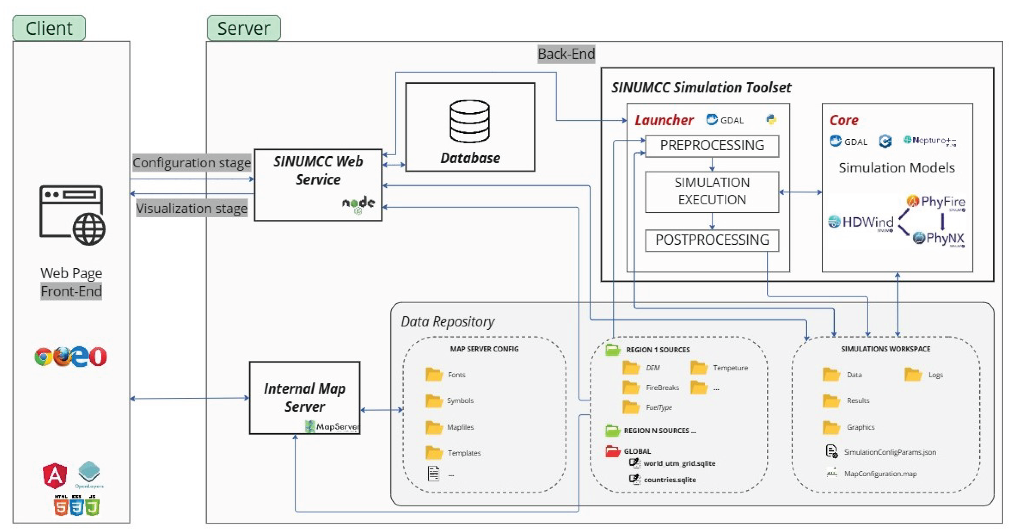
Figure 2.
Diagram of the coupling between three simulation models: HDWind, PhyFire, and PhyNX. three coupled models, and input and output data. Inputs include wind, temperature, humidity, DEM, fuel properties, and fuel moisture content. Outputs such as wind field and burned fuel feed into subsequent models, resulting in final outputs
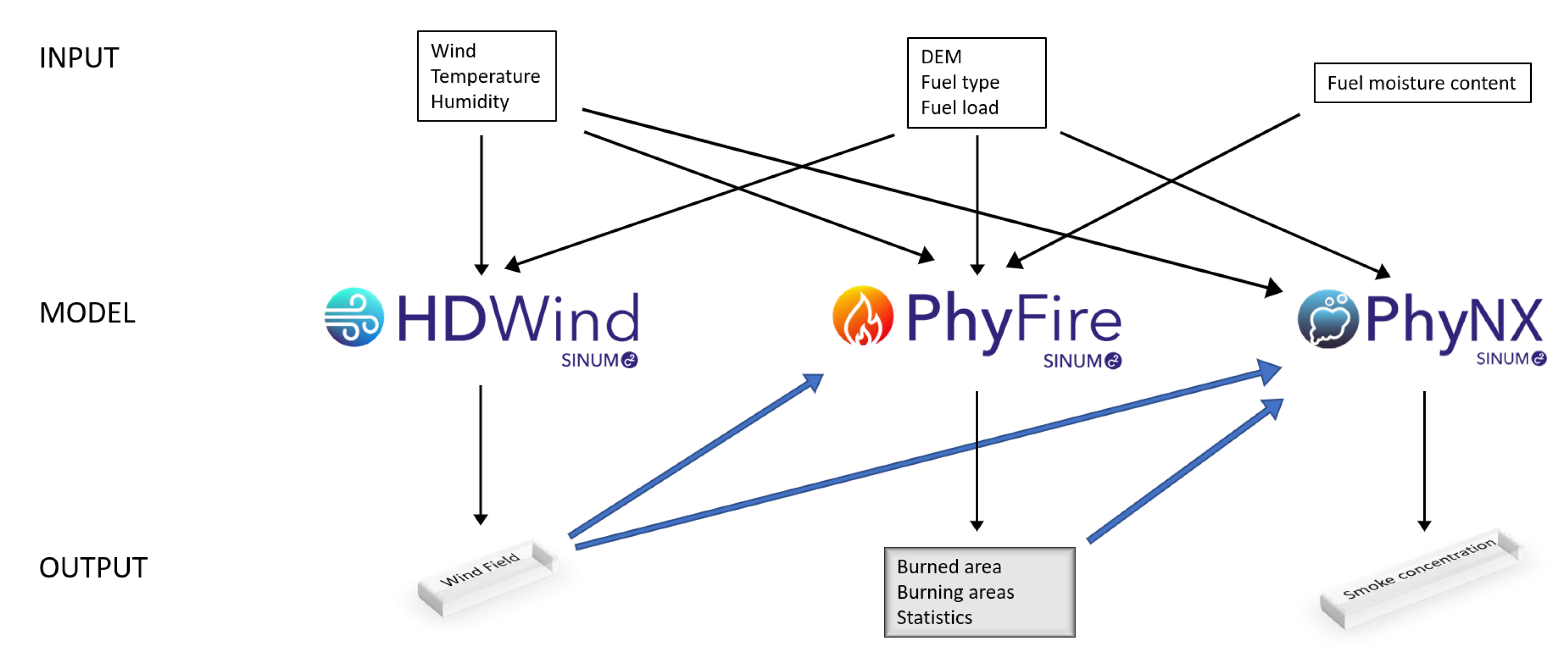
Figure 3.
Workflow of the three-stage workflow of the HDWind-PhyFire-PhyNX system: configuration, simulation, and visualization. Users define fire scenarios using geospatial, meteorological, and fuel data. The Neptuno Core handles simulation processing, integrating HDWind, PhyFire, and PhyNX models. Results are visualized through maps, statistics, and 3D animations, supporting wildfire analysis and decision-making
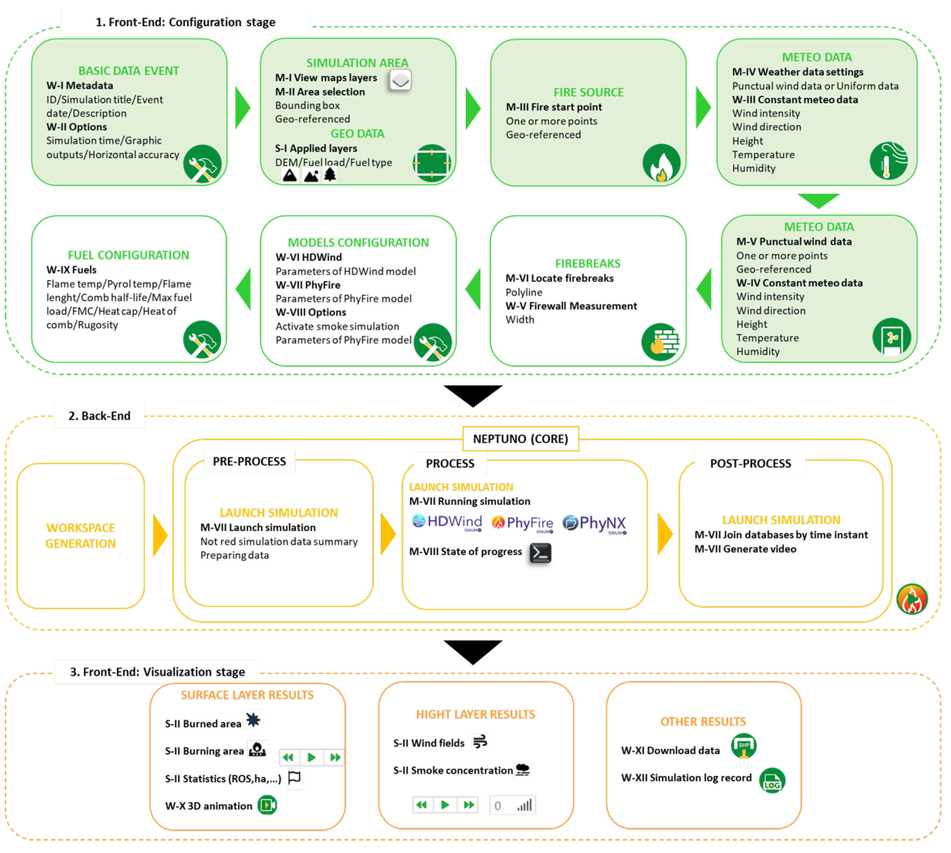
Figure 4.
Configuration interface for defining simulation metadata and general options. (a) Metadata tab, where the simulation title, description, and start date are entered. (b) Options tab, used to set the simulation duration, spatial resolution, and output interval.
Figure 4.
Configuration interface for defining simulation metadata and general options. (a) Metadata tab, where the simulation title, description, and start date are entered. (b) Options tab, used to set the simulation duration, spatial resolution, and output interval.
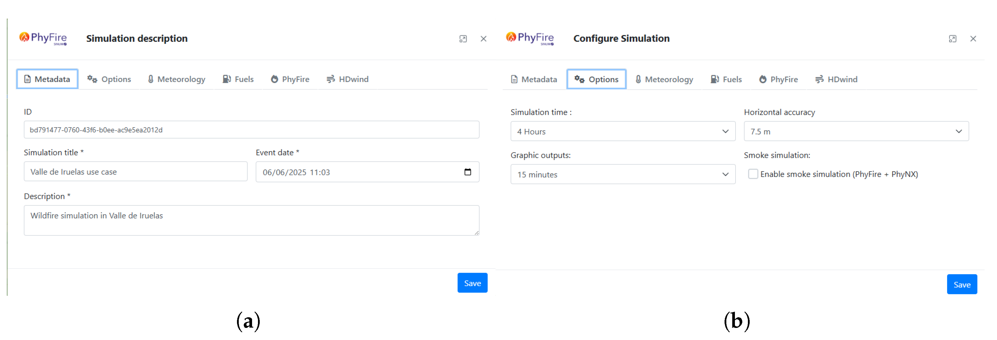
Figure 5.
Selection of the simulation area using different base and thematic layers available in the WebGIS interface. (a) Fuel type and fuel presence maps. (b) Very high resolution (VHR) satellite imagery [47]. (c) Spanish National Plan for Aerial Orthophotography (PNOA) [48]. (d) OpenStreetMap (OSM) base layer [49].
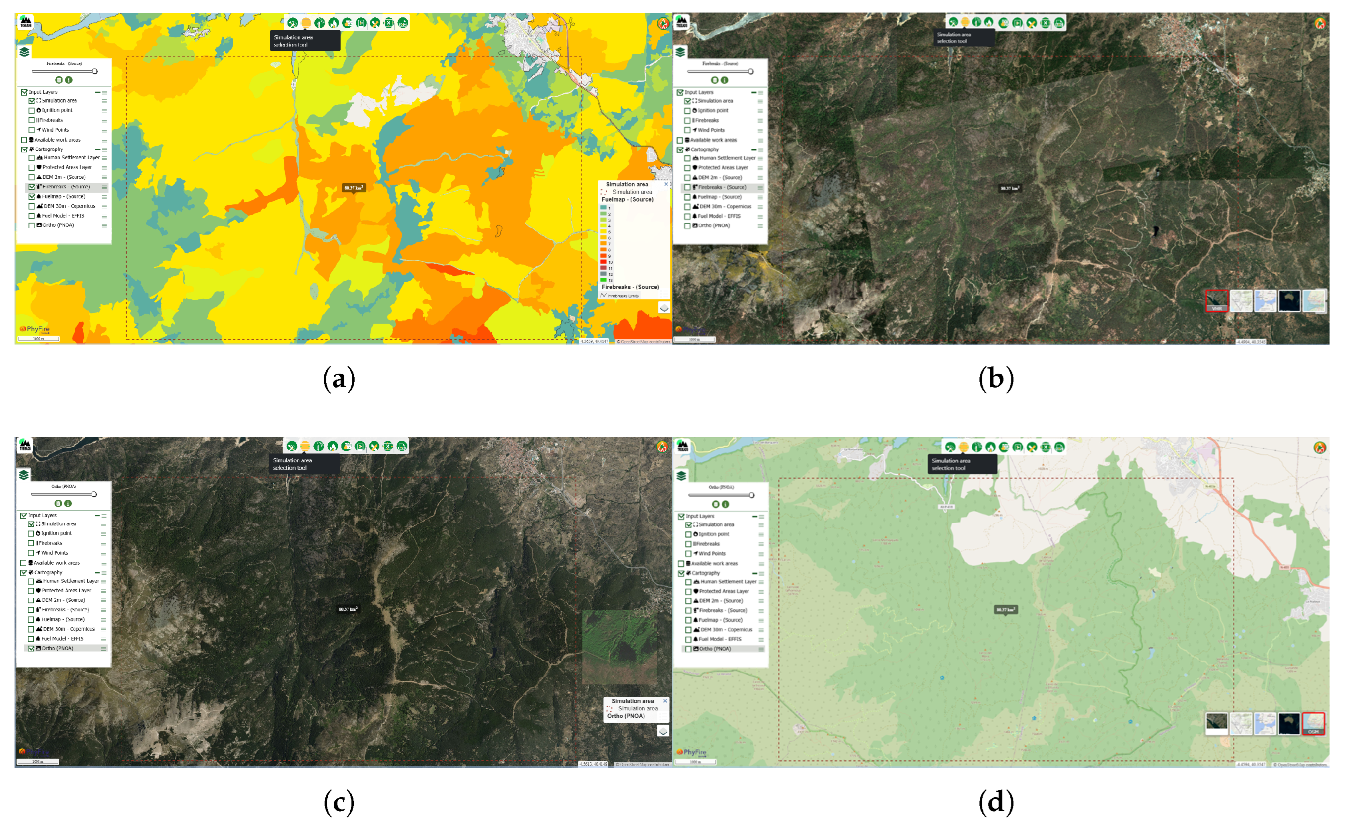
Figure 6.
(a) Ignition point displayed on the base map. (b) Manual input of hourly uniform wind data. (c) Selection of the “Punctual Wind Data” option and visualization of the meteorological reference point. (d) Example of a firebreak drawn in the simulation area.
Figure 6.
(a) Ignition point displayed on the base map. (b) Manual input of hourly uniform wind data. (c) Selection of the “Punctual Wind Data” option and visualization of the meteorological reference point. (d) Example of a firebreak drawn in the simulation area.
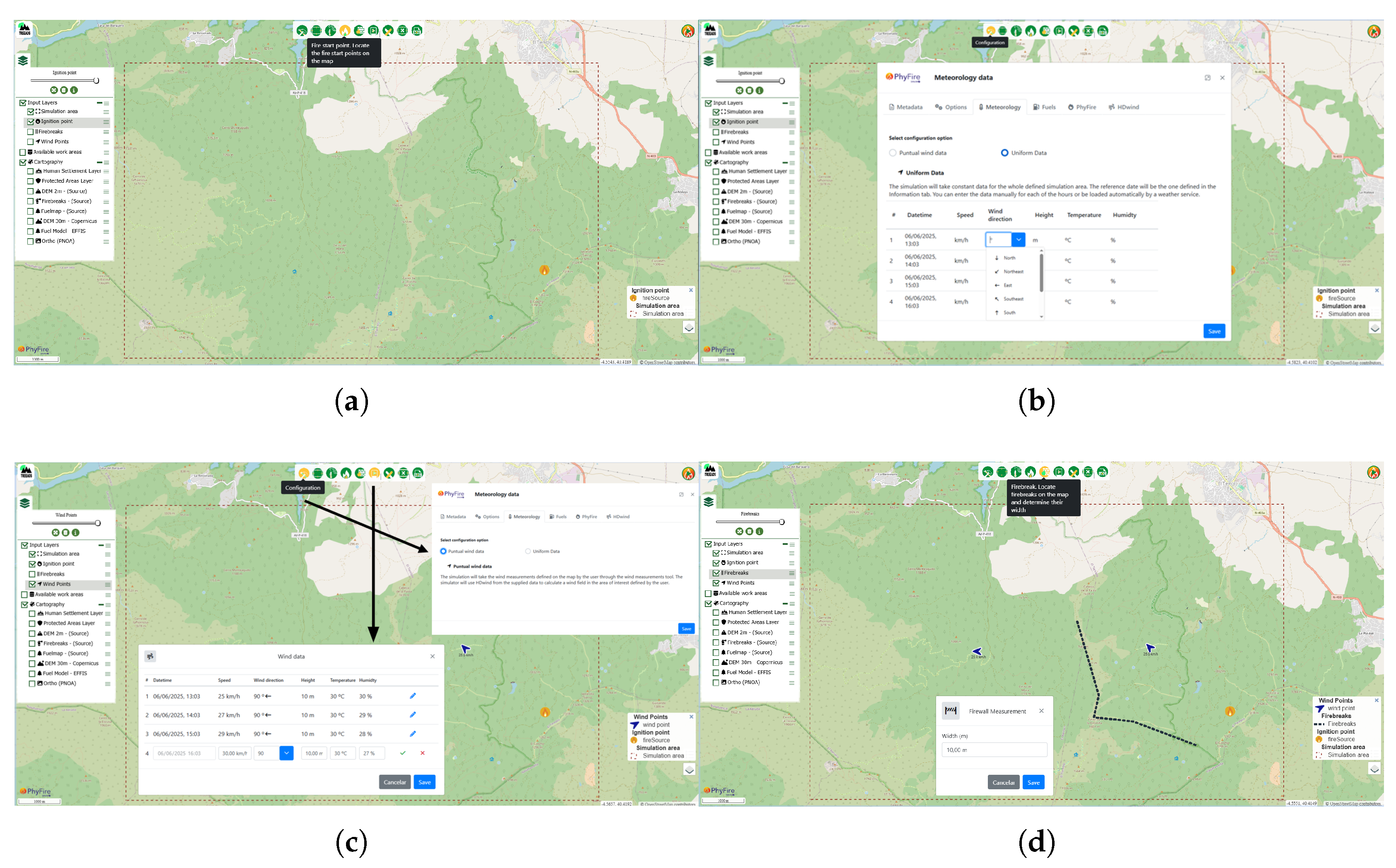
Figure 7.
(a) Fuel-type-dependent parameters. (b) Configuration panel for HDWind model parameters. (c) PhyFire model parameters, including fire-spotting option. (d) PhyNX model parameters, displayed when smoke simulation is enabled.
Figure 7.
(a) Fuel-type-dependent parameters. (b) Configuration panel for HDWind model parameters. (c) PhyFire model parameters, including fire-spotting option. (d) PhyNX model parameters, displayed when smoke simulation is enabled.
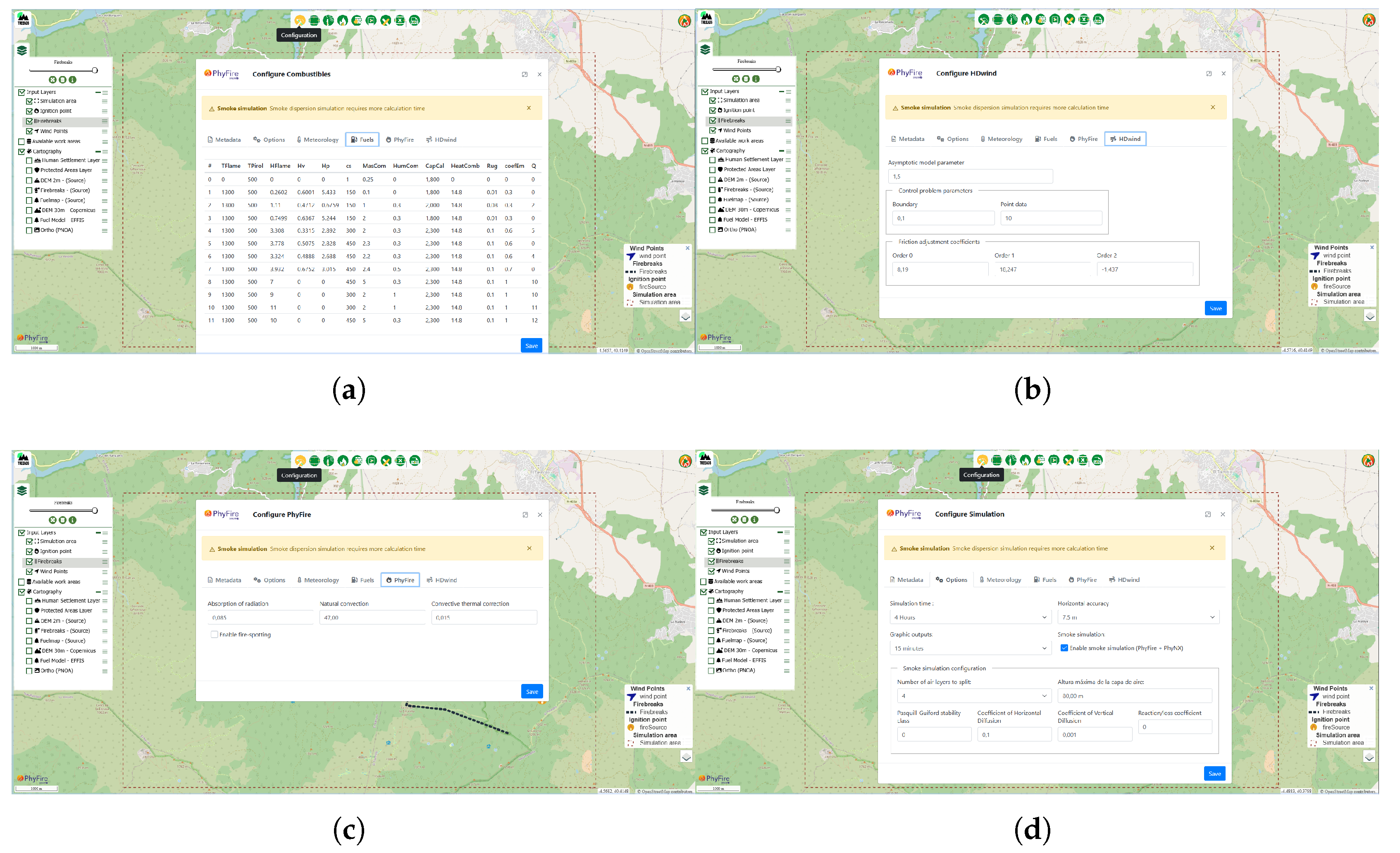
Figure 8.
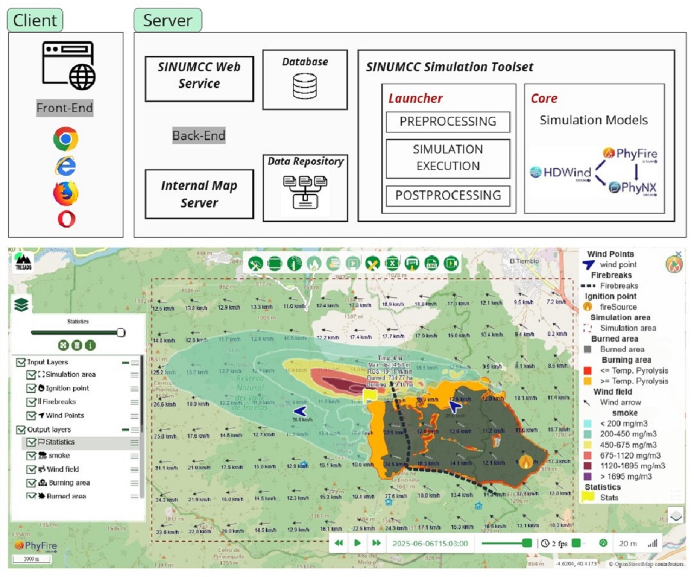
Visualization outputs from the WebGIS platform corresponding to the simulation results. (a) Simulated wind field. (b) Burned and burning areas with associated fire spread statistics. (c) Smoke concentration at ground level (0 meters). (d) Smoke concentration at 20 meters above ground level. The 10-meter-wide firebreak effectively halts lateral fire spread but fails to stop head fire advancement. Smoke plume dispersion is governed by the wind field simulated using the HDWind model.
Figure 8.
Visualization outputs from the WebGIS platform corresponding to the simulation results. (a) Simulated wind field. (b) Burned and burning areas with associated fire spread statistics. (c) Smoke concentration at ground level (0 meters). (d) Smoke concentration at 20 meters above ground level. The 10-meter-wide firebreak effectively halts lateral fire spread but fails to stop head fire advancement. Smoke plume dispersion is governed by the wind field simulated using the HDWind model.
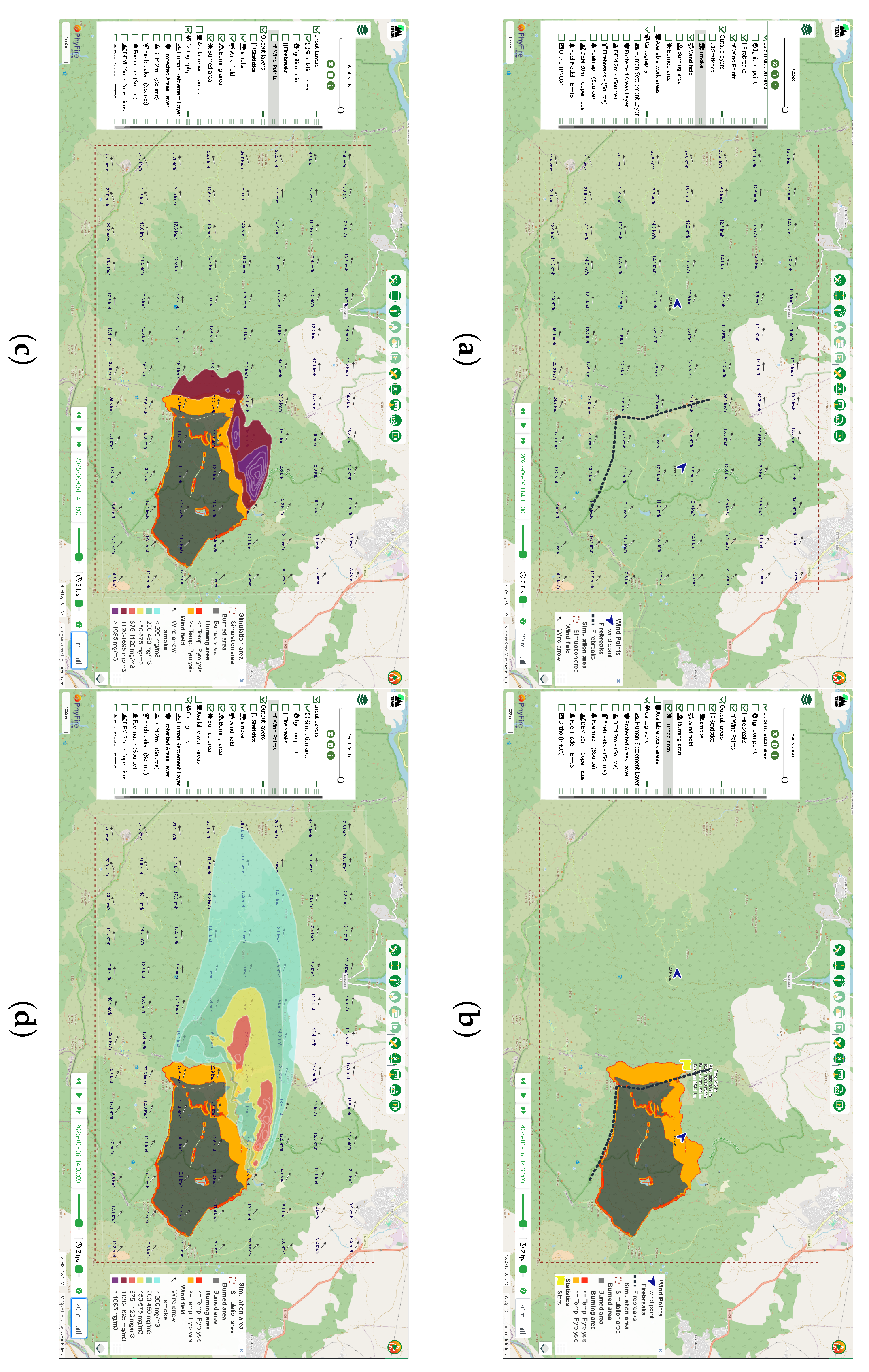

Table 1.
Model parameters. The table lists the parameters used in different sub-models (column Model) along with their physical meaning (Parameter), corresponding symbol (Symbol), and units of measurement (Units). Parameters are grouped into main parameters and fuel type dependent parameters
Table 1.
Model parameters. The table lists the parameters used in different sub-models (column Model) along with their physical meaning (Parameter), corresponding symbol (Symbol), and units of measurement (Units). Parameters are grouped into main parameters and fuel type dependent parameters
| MAIN PARAMETERS | |||
|---|---|---|---|
| Model | Parameter | Symbol | Units |
| HDWind | Buoyancy force coefficient | − | |
| HDWind | Smoothing function coefficient | − | |
| HDWind | Regularization term coefficient | − | |
| PhyFire | Radiation absorption coefficient | a | |
| PhyFire | Convective correction factor | − | |
| PhyFire | Natural convection coefficient | H | |
| PhyNX | Horizontal dispersion coefficient | ||
| PhyNX | Vertical dispersion coefficient | ||
| FUEL TYPE DEPENDENT PARAMETERS | |||
| Model | Parameter | Symbol | Units |
| HDWind | Roughness index | m | |
| PhyFire | Heat capacity | C | |
| PhyFire | Maximum initial fuel load | ||
| PhyFire | Fuel moisture content | water fuel | |
| PhyFire | Maximum flame temperature | K | |
| PhyFire | Pyrolysis temperature | K | |
| PhyFire | Combustion half-life | s | |
| PhyFire | Flame length independent factor | m | |
| PhyFire | Flame length wind correction factor | ||
| PhyFire | Flame length slope correction factor | − | |
| PhyNX | Emission factor | − | |
Disclaimer/Publisher’s Note: The statements, opinions and data contained in all publications are solely those of the individual author(s) and contributor(s) and not of MDPI and/or the editor(s). MDPI and/or the editor(s) disclaim responsibility for any injury to people or property resulting from any ideas, methods, instructions or products referred to in the content. |
© 2025 by the authors. Licensee MDPI, Basel, Switzerland. This article is an open access article distributed under the terms and conditions of the Creative Commons Attribution (CC BY) license (http://creativecommons.org/licenses/by/4.0/).
Copyright: This open access article is published under a Creative Commons CC BY 4.0 license, which permit the free download, distribution, and reuse, provided that the author and preprint are cited in any reuse.


