

Submitted:
30 June 2025
Posted:
02 July 2025
You are already at the latest version
Abstract
This paper primarily investigates the solutions to the system of matrix equations $A_1 X B_1 = C_1$ and $A_2 X B_2 = C_2$. This system generalizes the classical equation $AXB = C$, as well as the system of equations $AX = B$ and $XC = D$, and finds broad applications in control theory, signal processing, networking, optimization, and other related fields. Various methods for solving this system are introduced, including the generalized inverse method, the vec-operator method, matrix decomposition techniques, Cramer's rule, and iterative algorithms. Based on these approaches, the paper discusses general solutions, symmetric solutions, Hermitian solutions, and other special types of solutions over different algebraic structures, such as number fields, the real field, the complex field, the quaternion division ring, principal ideal domains, regular rings, strongly *-reducible rings, and operators on Banach spaces. In addition, matrix systems related to the system $A_1 X B_1 = C_1$ and $A_2 X B_2 = C_2$ are also explored.
Keywords:
system of matrix equations
; general solution
; special solution
; Moore-Penrose inverse
; vec-operator
MSC: 15A03, 15A09, 15A24, 15B33, 15B57, 65F10, 65F45
1. Introduction
The solution of linear matrix equations has garnered significant attention due to its wide-ranging applications in control theory [1,2,3,4], signal processing [5], computer vision [6], network analysis [7], machine learning [8,9,10], robotics [11], and optimization problems [12,13,14,15,16,17]. Previous studies have investigated various solution methods and associated numerical algorithms for the matrix equation
under different algebraic structures, and have discussed its applications in color image processing [18]. In contrast, [19] focused on several approaches for solving the system of matrix equations
and provided a comprehensive overview of the current state of research. Systems (1) and (2) can be regarded as special cases of the more general system
which introduces additional analytical and computational challenges. Compared to systems (1) and (2), the general form (3) involves an unknown matrix X that is simultaneously affected by multiple coefficient matrices on both the left and right. Moreover, the coupling of the two equations further complicates the analysis of solvability and the construction of explicit solutions.
On the other hand, the matrix system (3) captures the intricate interdependencies within systems governed by multiple variables and constraints, making its solution of considerable practical significance. In control systems, (3) is widely utilized for system identification, stability analysis, and optimal control design. Specifically, in the modeling and analysis of multi-input multi-output systems, it is frequently solved to extract system dynamics or determine controller design parameters [20]. Furthermore, such matrix systems play a vital role in signal processing, particularly in multidimensional signal processing, adaptive filtering, and joint estimation tasks [21]. In image processing and computer vision, the system (3) arises in applications such as image reconstruction, feature matching, and camera calibration [22,23], where the solution typically involves solving and integrating multiple matrix equations. Additionally, the matrix system (3) is fundamental in high-dimensional data analysis, machine learning, and large-scale optimization, as they contribute significantly to reducing computational complexity and enhancing algorithmic efficiency [24].
The problem of solving the matrix system (3) has garnered considerable attention from the research community, owing to its theoretical importance and wide range of practical applications. Over the years, numerous scholars have explored this system and related formulations, yielding a variety of results concerning existence conditions, solution structures, and computational strategies. As the field has matured, increasingly refined and effective methods have been proposed for analyzing and solving such matrix equations.
This paper presents a comprehensive review of several major classes of methods for solving the system (3), including generalized inverse techniques, -operator approaches, matrix decomposition strategies, Cramer’s rule, and numerical algorithms. Each class of methods offers distinct advantages and limitations depending on the underlying algebraic framework and the specific type of solution sought. A comparative summary of these methods is provided in Figure 1.
The structure of the paper is as follows: Section 2 introduces the notations used throughout the paper, along with preliminary concepts and definitions. In Section 3, we review various solutions to the matrix system (3) based on generalized inverse methods, which are among the earliest and most widely used approaches. Section 4 presents solutions derived using the -operator methods. Matrix decomposition methods for solving the system (3) over the complex field, as well as Cramer’s rule-based approaches over the quaternion algebra, are discussed in Section 5 and Section 6, respectively. Section 7 focuses on iterative methods for computing symmetric-type solutions of the system (3) over the real field. Finally, Section 8 provides concluding remarks and outlines potential directions for future research on solving the system (3).
2. Preliminaries
To facilitate the discussion in the following sections, this section introduces some preliminary concepts and definitions.
Throughout the text, let denote a field, represent the complex field, and denote the real field. The notations , , and refer to the sets of dimensional matrices over , , and , respectively.
The collections of quaternions, commutative quaternions (also known as reduced biquaternions), and split quaternions are defined as follows [25,26,27]:
Correspondingly, dimensional quaternion matrices, commutative quaternion matrices, and split quaternion matrices are denoted as , , and , respectively. For (or or ), the matrix A can be written as
where , and
where . From these definitions, it is clear that quaternions, commutative quaternions, and split quaternions are all four-dimensional Clifford algebras, but they differ in their multiplication properties. While all three are associative algebras, only commutative quaternions satisfy the commutative law. The study of these three quaternion types employs different methods, but they are interrelated. Additionally, only quaternions have an inverse for every nonzero element, making their study the most extensive. Tools such as the generalized inverse, rank, and matrix decomposition can be applied to solve systems over quaternions. In contrast, the study of commutative and split quaternions requires utilizing their representations and transforming them into the real or complex fields for analysis.
We use to denote a ring. Let represent the set of matrices over . A principal ideal domain is a ring in which every ideal is a principal ideal. A regular ring is one in which, for any element a in the ring, there exists an element , such that , also known as a von Neumann regular ring. In fact, a regular ring is one where every element has a right inverse, and this property allows the concept of a right inverse to play a crucial role in solving equations in regular rings. If for any , the condition implies , then is a *-reducing ring. A ring is strongly *-reducing if, for , , the equation implies for each . A Banach space is a complete normed linear space. Let E and F be Banach spaces. The set of operators that are both linear and bounded from E to F is denoted by .
The symbols I and 0 represent the identity matrix and the zero matrix, respectively. For matrices over a field, we denote the rank, image, and kernel of a matrix A as , , and . The rank of a matrix over quaternions can be defined in a similar way. For a principal ideal domain , if , then if there exists an nonzero minor of A, and every minor of A is zero. If , then G is called a right divisor of A, and A is referred to as a left multiple of G. The greatest right divisor of A is defined as the right divisor that is a left multiple of every right divisor of A.
For a matrix A, denotes the transpose of A, represents the conjugate of A, and denotes the conjugate transpose of A. Specifically, for a complex matrix , it can be expressed as , where , , and . For quaternion, commutative quaternion, and split quaternion matrices, A can be written as , where , , and . For matrices A and B, the inner product is given by . Additionally, represents the orthogonal projector onto the subspace . The symbols , and stand for the right column space, the right null space, the left row space, and the left null space of a matrix , respectively.
Next, we introduce some special matrices and their definitions. Let be the i-th column of the identity matrix of order n, and . Some definitions of special matrices are listed in Table 1, where .
Furthermore, assume that . If for and for , then A is called an indeterminate admittance matrix. If A is both Hermitian and an indeterminate admittance matrix, it is referred to as a Hermitian indeterminate admittance matrix, or HIA matrix.
Finally, we introduce the Hankel matrices, which are defined in the following form:
Denote as the collection of all Hankel quaternion matrices.
3. The generalized inverse methods
In 1954, Penrose introduced a generalization of the matrix inverse via the unique solution to four matrix equations:
where is referred to as the general inverse or the Moore-Penrose inverse of A [28]. In the subsequent discussion, we define the symbols and .
Remark 1.
The Moore-Penrose inverse exists uniquely for elements in the real field, the complex field, and the quaternion division ring.
As a special case of the Moore-Penrose inverse, Rao and Mitra introduced the concept of the inner inverse (g-inverse), which satisfies the equation:
where is defined as the g-inverse of A[29]. We define notations and .
Remark 2.
For any regular element in a ring, the inner inverse exists but is not necessarily unique.
Both the Moore-Penrose inverse and the inner inverse are fundamental tools for solving matrix equations. They can be applied in various algebraic structures, such as fields, skew fields, rings, etc., and also play a key role in providing explicit solutions to specific matrix equations.
This section is organized into two main parts: SubSection 3.1 discusses the application of generalized inverse methods in general fields, with particular emphasis on related results in the fields of complex and real numbers. SubSection 3.2 explores relevant results in the quaternion division ring, principal ideal domains, regular rings, strongly *-reducible rings, and Banach spaces. Additionally, this section examines solutions of special types, such as Hermitian solutions over the complex field, centro-symmetric solutions, and P-anti-symmetric solutions over the quaternion division ring. The computation of these special solutions often involves solving more complex systems of equations.
3.1. The general, complex and real fields
The solution to the system (3) over general fields was first presented by Mitra in 1973 using the g-inverse [30]. Subsequently, Woude provided various characterizations of solvability conditions, including rank and null space criteria, and extended these results to more complex systems [31,32,33,34]. In 1988, John offered a more concise expression for the general solution to the system (3) [35]. Following decades of development, the least-squares solution representation for the system (3) over the complex field was introduced in 2011 and later applied to the Hermitian solution of the system [36]. Moreover, He, Wang, and others progressively investigated solutions for systems with three and four equations over the complex field [37,39]. In 2020, researchers employed projection operators to provide alternative representations of the system (3) [38].
In 1973, Mitra first provided the necessary and sufficient conditions for the solvability of the matrix equation system (3) and the explicit expression for its solution [30].
Theorem 1 (General solutions for (3) over [30]). Assume that and . A necessary and sufficient condition for the system of equations (3) to be consistent is
In this case, the general solution is
where U is arbitrary, Y and Z satisfy
and
In 1987, Woude studied measurement feedback for non-interacting control systems. He characterized the conditions for the solvability of the system in terms of ranks, null spaces, and column spaces of matrices [31,32]. Three years later, Mitra, using block matrices, introduced an additional equivalent condition for solvability and provided an explicit expression for the solution when it exists [33]. Their conclusions are summarized in Theorem 2.
Theorem 2 (General solutions for (3) over [31,32,33]). Suppose that and . The system is consistent if and only if the following conditions hold:
For , , , and
For , , , and
For matrices Y and Z properly chosen and fixed, the equation
is consistent.
For , , , and
where , , , and satisfy the conditions
and
When any one of the conditions - holds, the general solution to the system of matrix equations is given by
where the matrix U is arbitrary, and Y, Z are general solutions to
and
Woude extended his own result in Theorem 2, by considering the following matrix equation system
where , , and are given matrices, and denotes a set of index pairs [34]. The solvability of the system is divided into two parts: , and , where for an arbitrary integer . The following conclusions are derived.
Denote
There exists a matrix X such that if and only if
for any .
Under the assumption that
there exists a matrix X such that for if and only if
for , and
Remark 3.
The consistency condition can be written in an equivalent form as
Similarly, the second solvability condition in Theorem 3 can also be expressed in terms of ranks.
Remark 4.
For , the assumption always holds. Indeed, in this case, both the left-hand side and the right-hand side are equal to . In this scenario, Theorem 3 can be deduced from Theorem 2.
Remark 5.
When
To obtain the expression for the solution of the system (3) using Theorems 1 and 2, two additional matrix equation systems need to be solved. Furthermore, [35] provides a more specific expression for the solution of the system (3).
Theorem 4 (General solutions for (3) over [35]). Let and . The system (3) has a general solution X if and only if the conditions
and
hold.
At this point, the form of the general solution X is given by
for arbitrary U with appropriate size.
In 2011, Liu and Yang obtained an explicit representation of the general least-squares solution to the system (3) over the complex field. Furthermore, this result was used to determine the conditions for the existence of a Hermitian least-squares solution to the matrix equation [36].
Define
Then, the matrix equation system (3) has a least-squares solution if and only if
Under this circumstance, the general least-squares solution can be expressed as
or equivalently,
where and are arbitrary matrices with appropriate sizes.
Suppose that the equations and are consistent, respectively. Denote
Then, (3) has a solution if and only if
To consider the least-squares solution to , Liu and Yang presented the solvability condition for the system
building upon Theorem 5 [36].
The matrix equation system (11) has a general least-squares solution if and only if the following rank condition holds:
When this condition is satisfied, the general least-squares solution of (11) can be expressed as
where
U, V, W and Z are arbitrary matrices with appropriate sizes.
If the equations and are consistent, then the system of matrix equations (11) is solvable if and only if
In this case, the general Hermitian solution can be expressed as (12), where
U, V, W and Z are arbitrary.
Remark 6.
Corollary 1 provides the consistent conditions and explicit expressions for the least-squares solution X to the system (11). Moreover, the Hermitian solution to can be derived from the general solution and is given by
where X is the solution of (11).
In 2013, He and Wang considered the more comprehensive system of matrix equations
over using the inner inverse [37]. The results are stated as follows:
and
Then, the system (13) has a solution if and only if
for , and
At this point, the general solution to (13) is
or equivalently,
where
with arbitrary for .
As applications of Theorem 6,37] also derived the Hermitian solutions of the systems
and
respectively. The related results are summarized in the following corollaries.
and
Then, the system (14) has a Hermitian solution if and only if
for , and
In this case, the Hermitian solution to (14) can be expressed as
with
or equivalently,
where
and are arbitrary.
and
Then, the system (15) has a Hermitian solution if and only if
In this case, the general solution to the system (15) can be expressed as
with
or equivalently,
where
and ) are arbitrary matrices with appropriate sizes.
Recently, Zhang et al. introduced a simple method to solve the system(3) using the orthogonal projector method [38]. Recall that for a subspace , denotes the orthogonal projector onto .
Then, the system (3) has a general solution if and only if
where and .
In this case, the general solution to the equations is given by
or equivalently,
where , , , are arbitrary matrices.
At the end of this subsection, we present the most general form of the result for to date. In 2021, the consistency conditions and solutions for the system of matrix equations over were proposed [39]:
As special cases of , the related results of and the system
are also presented in [39].
for . Let
The system of equations is consistent if and only if
One of the following systems of matrix equations is consistent:
where
For some solution of , the following system is solvable by , W, , and Z:
Or equivalently, for , where X is a solution of , the following two equations are separately solvable by , W, , and , respectively:
where
In these cases, the general solution of can be expressed as
where
and is a solution of , and are
for some and satisfying and , with arbitrary , and Z.
Replace some symbols in Theorem 8, and the corollaries regarding (13) and (17) are provided by [39].
3.2. Various rings and the quaternion algebra
Research on the system (3) over rings began with principal ideal domains possessing special properties [40]. Later, Wang observed that the results related to the g-inverse on regular rings could also be similarly generalized [41]. He progressively explored more complex systems with two unilateral constraints and two bilateral constraints, extending these results to simpler equations, including centro-symmetric and P-(anti-)symmetric forms [42,43,44]. In 2015, the general solution to the system (3) was also derived for operators on associative rings with identity, strongly *-reducible rings, and Banach spaces [45].
Özgüler and Akar obtained the necessary and sufficient condition for the existence of the solution to the system (3) over a principal ideal domain [40]. The solvability condition of (3) over is that the equations each have a solution and a constructed bilateral linear matrix equation has a solution. The specific conclusions are as follows:
Theorem 9 (General solutions for (3) over principal ideal domains [40]). For a principal ideal domain , assume that , , , , , and . Let , , , and be unimodular matrices such that
where , are of full row rank and , are of full column rank. Denote
partitioned such that and . Additionally, suppose that , are the greatest left divisors of , , and , are the greatest right divisors of , , respectively, such that
for some left unimodular , and right unimodular , . Define and as
Then, the system (3) has a solution X over if and only if the following conditions hold:
(1) , , for .
(2) for .
(3) There exist , , , and such that
Remark 7.
Under this condition, Theorem 9 reduces to Theorem 2.
From 2004 to 2008, Wang and his collaborators conducted a series of studies, presenting results for the system (3) in regular rings and quaternion skew fields [41,42,43,44]. In a regular ring, where every element possesses an inner inverse, expressing the solution to the system (3) using the inner inverse becomes a natural consequence.
We recall the analogous relations over the regular ring . For , , and , we denote the following similarity relation:
if there exist invertible matrices and such that
Using this similarity relation, Wang derived the necessary and sufficient conditions for the solvability of the system (3) in the regular ring , as well as an explicit expression for its solution [41].
Theorem 10 (General solutions for (3) over regular rings [41]). For a given regular ring , let , , , , , and . Denote , , , and . Then the following conditions are equivalent:
The system is consistent.
The equations
and
hold for .
The following similarity relations:
hold for .
In that case, the general solution of the system can be expressed as
where Y and W are any matrices over with appropriate dimensions.
Remark 8.
Matrix similarity in a regular ring is defined similarly to matrix similarity in a general domain. However, unlike in a field, matrix similarity in a regular domain cannot be defined using rank equality. Instead, it can be expressed in terms of the inner inverse.
In 2005, Wang considered as an extension of the system over quaternion algebra. He provided a necessary and sufficient condition for the existence of the general solution to the system [42].
Then, the system is consistent if and only if
and
At this point, the general solution of can be expressed as
with arbitrary matrices W and Z over .
In the same year, Wang also studied the centro-symmetric solutions to the following system of matrix equations over :
where the solutions were explicitly derived in [43]. In this context, for a given matrix , the notation is used to denote the matrix obtained by reversing the row and column indices of A.
Then, there exists a centro-symmetric solution to the system if and only if
and
hold.
Under these conditions, the centro-symmetric solution of can be expressed as
where
with arbitrary matrices over .
Remark 9.
The consistency of the system for a centro-symmetric solution is equivalent to the solvability of the following system:
which corresponds to the general solutions. Hence, the proof of Theorem 12 follows directly from the results of Theorem 11.
In 2008, Wang et al. established the solvability conditions and expressions for the P-(anti-)symmetric solutions to the system of matrix equations [44].
Theorem 13
(P-(anti-)symmetric solutions for (23) over [44]). Assume that , and are given matrices. Suppose a nontrivial involution P is expressed as
Define the following partitions:
Let , , , , , and . Then, the system (23) has a P-(anti-)symmetric solution if and only if
Equations
hold.
Rank conditions
are all satisfied.
Under these conditions, the P-symmetric or P-anti-symmetric solution X can be expressed as
or
where , are given by
Here, Y, V, W and Z are arbitrary matrices.
Dajić studied the system over associative rings with a unit, strongly *-reducible rings, and operators between Banach spaces. The necessary and sufficient conditions for the existence of solutions, as well as expressions for the general solutions, were derived [45].
Theorem 14 (General solutions for (3) over associative rings with a unit [45]). For an associative ring with a unit. Let , , , , , and . Assume that are regular. Denote
where are regular.
The system is solvable if and only if the equation
is consistent for some .
When , is consistent if and only if there exist such that
If and , then the system (3) has a general solution if and only if
If one of the above conditions holds for (3), then the general solution can be expressed as
where
and and Z arbitrary elements of . It worth noting that and can be simplified to and , respectively.
Theorem 15 (General solutions for (3) over strongly *-reducing rings with a unit [45]). For a strongly *-reducing , assume that , , , , , and , where and are regular. If the conditions of Theorem 14 hold, the general solution to is given by
where is arbitrary, are as defined in and .
Theorem 16 (General solutions for the operator system (3) between Banach spaces [45]). Suppose that be Banach spaces. Given , , , and assume that
are regular. If and , then the system of equations has a general solution if and only if
In this case, the general solution is given by
where
and Z are arbitrary elements of , and , respectively.
Remark 10.
Naturally, Theorem 16 can be extended to matrices over . The specific conclusions are identical to those in Theorem 16, so they will not be repeated here.
In this section, we have introduced the generalized inverse method for solving the system (3). As one of the earliest and most widely used approaches for this class of problems, the generalized inverse method provides a fundamental framework for deriving solutions. Most of the subsequent methods discussed in this dissertation are either extensions of, or closely related to, the generalized inverse approach.
4. The -operator methods
In this section, we present the method for solving the system (3) involving the vector operators. First, we introduce the definition of the -operator and its related properties.
Let be an matrix, where for . The -operator of A is defined as
where the vector consists of the columns of the matrix A stacked on top of each other.
Remark 11.
The -operator is both a bijection and a linear mapping.
The inverse operator of A can also be defined. For an -dimensional vector , we use the notation to denote the matrix A such that .
Next, we define the Kronecker product of two matrices. For an matrix and a matrix B, the Kronecker product of A and B is given by
which results in a matrix of order .
The vector operators have broad applications in solving various systems of equations, primarily because they satisfy the following properties in the complex domain. Let , , and . Then, the following identity holds:
Using this result, complex systems of linear equations, including (3), can be transformed into the form .
For quaternions, commutative quaternions, and split quaternions, their real or complex representations can be employed to convert them into real or complex systems of equations for further solution. Additionally, specialized vector operators can be designed for different types of solutions, ensuring that when the matrix is recovered, it retains the properties of a special matrix.
Finally, for the equation , the following lemma provides the solvability conditions and the expression for the general or least-squares solution using the Moore-Penrose inverse.
Lemma 1.
When the equation is consistent, the general solution is given by
where is arbitrary. If the matrix equation is inconsistent, then the least-squares solution is given by
This form provides the unique minimal norm general or least-squares solution.
This section is organized into several parts. We begin by discussing the solution of the system (3) in the complex domain using the -operator. Following that, we explore the solutions in the quaternion ring, including Hermitian, -bi-Hermitian, (anti-)centro-Hermitian, and Hankel solutions. Lastly, we address the -Hermitian solution for split quaternions and the Hermitian solution for commutative quaternions.
4.1. The complex field
The concept of using vector operators to solve the system (3) was first introduced by Navarra in 2001 [47]. Subsequently, scholars recognized that vector operators could be designed for symmetric, anti-symmetric, and bi-symmetric matrices, which led to the exploration of special solutions for (3). As a result, from 2016 to 2018, the least-squares Hermitian solution and Hermitian indeterminate admittance solution of (3) were extensively studied [48,49,50].
In 2001, Navarra et al. derived necessary and sufficient conditions for the existence of a general solution to (3) and presented an expression of the general solution using the -operator and -operator [47]. This marked the first application of the in solving the system (3).
Theorem 17 (General Solutions for (3) over [47]). Suppose that , , and are known matrices. The system of matrix equations (3) is consistent if and only if
and
where , , , and .
If the general solution to (3) exists, the expression for the general solution is given by
with arbitrary .
Remark 12.
Recall the fact that the matrix equation has a Hermitian solution if and only if the pair of matrix equations (11) has a general solution X. The Hermitian solution of can be represented as
Baaed on this result, [47] presents the consistent condition and expressions of the Hermitian solution of .
Fifteen years later, the least-squares Hermitian solution with the minimum-norm of (3) has been considered. [48] directly focused on the properties of complex Hermitian matrices, designing and operators for symmetric and anti-symmetric matrices to describe the real and imaginary parts of Hermitian matrices.
For a matrix , the operator is defined as
The operator is denoted as
Let , , and , where (). Define the circle product satisfying the following conditions.
.
.
For , where and other elements of E are zeros, define
and
With the above definitions, an equivalent characterization of Hermitian matrices is given as follows. For a square real matrix , X is a symmetric matrix if and only if
and X is an anti-symmetric matrix if and only if
Hence, for a complex square matrix , X is a Hermitian matrix if and only if
Based on above results, the main theorem of [48] is given.
Theorem 18 (Hermitian solutions for (3) over [48]). Let , , , , , . Define the complex matrices , , , and for as
where , are the i-th column vectors of matrices and , and , are the j-th row vectors of matrices and , respectively. For , define
Let
The system (3) is consistent for Hermitian solutions when
Then, the Hermitian or least-squares Hermitian solution of (3) is of the form
where is an arbitrary vector. The system (3) has a unique minimum-norm Hermitian or minimum-norm least-squares Hermitian solution satisfying
Solving the system (3) using Theorem 18 involves the operation of the inner product of the matrix, which is computationally expensive. [50] uses real representation to transform the problem in the complex number field into the real field, improving the effectiveness of the method.
Define as the i-th column of . Let be
and be
The symbols and present another equivalent characterization of Hermitian matrices. For a real square matrix , X is a symmetric matrix if and only if
X is an anti-symmetric matrix if and only if
Thus, for a complex square matrix , X is a Hermitian matrix if and only if
Additionally, the definition of the real representation of a complex matrix is presented. For a complex matrix , where , denote
and
Assume , then , where
with
Based on the real representation of complex matrices, [50] presents another expression of the consistent conditions and expressions for the general and least-squares solutions for (3).
and
The system (3) is consistent when
Then, the general or least-squares solution of (3) is of the form
where is an arbitrary vector. The system (3) has a unique minimal norm general or least-squares solution satisfying
Remark 13.
Based on the real representation of complex numbers, the system of matrix equations (3) is equal to
Remark 14.
Compared to Theorem 18, Theorem 19 does not involve complex number operations, resulting in improved computational efficiency. This conclusion is also verified by the numerical experiments presented in [50].
Later, Hermitian indeterminate admittance (HIA) solutions of the system (3) have been considered by Liang et al. [49].
For describing Hermitian indeterminate admittance matrices, [49] designed operators and . For , denote
and
On the other hand, let
and
For a square real matrix , X is a symmetry matrix if and only if
and X is an anti-symmetry matrix if and only if
Hence, for a complex square matrix , X is a Hermitian matrix if and only if
The results of [49] presenting the consistency conditions of (3) having HIA solutions are as follows:
where , is the i-th column vector of matrix and , , is the j-th row vector of matrix and , respectively. Let
where ,
Then, the system (3) has a Hermitian indeterminate admittance solution X if and only if
At this point,
with arbitrary Y.
Liang et al. have presented an another method of solving the Hermitian indeterminate admittance of (3) [49].
For for , let
and
Then, assume that , then A is a symmetry indeterminate admittance matrix if and only if
and A is an anti-symmetry indeterminate admittance matrix if and only if
Hence, for a complex matrix , then A is a Hermitian indeterminate admittance matrix if and only if
Naturally, the following theorem holds.
Then the existence conditions of the Hermitian indeterminate admittance solution X of (3) can be expressed as
In this case, X satisfies
with arbitrary Y.
In the process of considering special solutions using vector operators over the complex number field, it is essential to treat the real and imaginary parts separately. In the following subsection, we demonstrate that when applying these methods to find special solutions over the quaternion field, the four components of quaternions must be addressed individually.
4.2. The quaternion algebra
This subsection considers the system (3) over quaternions with general and various Hermitian solutions. It is well known that quaternion algebra is non-commutative, which means that the equation (26) does not hold over . However, with the help of the quaternion complex representation, the least-squares Hermitian, -bi-Hermitian, (anti-)centro-Hermitian, and Hankel solutions for (3) can all be derived [51,52,53,54,56]. Additionally, the (anti-)centro-Hermitian solution of (3) was also considered using its real representation [55].
We first introduce the complex representation and related properties for quaternions. Any quaternion matrix can be represented as where . Denote , , and
Remark 15.
For , , and , the following conclusions can be derived:
,
,
,
.
Thus, Φ, Ψ, and f are linear maps.
Based on the real representation, Kronecker product, and the equation (26), the -operator over quaternions can be described.
Lemma 2
Based on different definitions of special matrices, the expression
has corresponding structures, which can be used to simplify the system (3) into the form .
To derive the general solution and least-squares solution, [51] introduces the below symbols. For a matrix , define the following vectors:
and
The and operators can also be used to express the symmetry and anti-symmetry matrices. Suppose , then:
, where is given by
, where the matrix is given by
Remark 16.
and are standard column orthogonal matrices, which satisfy
respectively.
Notice that for to be Hermitian, it must satisfy that
Hence, X satisfies
The main results of [51] can be presented as follows:
and
The quaternion matrix system (3) has a Hermitian solution if and only if
Then the Hermitian solution of (3) can be expressed as
with an arbitrary real vector y.
The unique Hermitian solution can be expressed as
When (3) is inconsistent, the least-squares solutions satisfy
where y is an arbitrary real vector.
Yuan et al. have considered the more complex -anti-Hermitian solution and -anti-bi-Hermitian solutions [52].
The operator for is designed for bi-symmetry matrices, with the following definition:
When is even, for the given matrix , define
When is odd, for , define
Similarly, the operator for is designed for anti-bi-symmetry matrices, defined as follows:
If , for , define
If , for , define
Suppose , then
where is given by
when , with order ;
when , with order .
Additionally,
where is given by
when , with order ;
when , with order .
Furthermore, if and only if and
if and only if and
Therefore, assume that , then
where
where
Theorem 23
Additionally,
The quaternion matrix system of equations has a solution if and only if
Under this circumstance, X is expressed as
where y is an arbitrary real vector with appropriate dimensions.
In this situation,
Furthermore, the least-squares solutions of (3) are in the form of
where y is an arbitrary real vector with appropriate dimensions. The unique minimum-norm least-squares solution is given by
Theorem 24
Furthermore,
The quaternion matrix system of equations has a solution if and only if
In this case,
where y is an arbitrary real vector with appropriate dimensions.
Under this circumstance,
Remark 17.
The η-Hermitian and η-anti-Hermitian solutions of (3) can also be derived using similar methods.
Remark 18.
Theorem 25 ((Anti-)centro-Hermitian solutions for (3) over [54]). Let , , , , , , and be given matrix. Denote
The least-squares (anti-)centro-Hermitian solution of (3) can be expressed as
with arbitrary vector h of suitable size.
For given , the optimization problem , with satisfying (3), has a unique solution X such that
where or for centro-Hermitian or anti-centro-Hermitian solutions.
Remark 19.
If the matrix is not (anti-)centro-Hermitian, then instead of the matrix , the expression
can be used to derive the (anti-)centro-Hermitian solutions of .
Later, Zhang et al. researched the (anti-)centro-Hermitian solutions for (3) through the real representation matrices of quaternion matrices [56].
A kind of isomorphic real representation of quaternion matrices is defined for a as
The first column of is denoted as
To describe the structure of (anti-)centro-Hermitian matrices using the real representation, the and is denoted as follows:
When
where for and for
If ,
where for and for .
If ,
with for
If ,
with for .
When ,
where for and for
When ,
where for and for
If ,
with for
If ,
with for .
The and operators present equivalent conditions for centro-Hermitian and anti-centro-Hermitian matrices. Let . Then
and
where
with
and
Then another result for the (anti-)centro-Hermitian solutions of (3) is yielded.
Then, the quaternion matrix equation system (3) has a centro-Hermitian solution if and only if
When (3) is consistent with centro-Hermitian solutions, these solutions can be expressed as
where y is arbitrary.
Moreover, if (3) has a centro-Hermitian solution, then the centro-Hermitian solution is unique if and only if
The unique centro-Hermitian solution is given by
Then, the quaternion matrix equation system (3) has an anti-centro-Hermitian solution if and only if
When (3) is consistent with anti-centro-Hermitian solutions, these solutions can be expressed as
where y is arbitrary.
Moreover, if (3) has an anti-centro-Hermitian solution, then the anti-centro-Hermitian solution is unique if and only if
The unique anti-centro-Hermitian solution is given by
At the end of this subsection, we introduce the Hankel solution of the quaternion matrix system of equations (3). Through a novel vector operator for Hankel matrices, [55] transforms the problem of finding Hankel solutions into solving for the general solutions. Then, the necessary and sufficient conditions for the system (3) with Hankel solutions, as well as the expression for the general solution, are derived.
A Hankel matrix
is uniquely determined by elements. Let
and
Then, for ,
and
There is a Hankel matrix solution of (3) if and only if
When such conditions is satisfied, the general Hankel matrix solution is
with arbitrary
There does not exist a Hankel matrix solution of (3), the least-squares Hankel solution is expressed as .
For a given , the solution of the optimal problem , with X is the Hankel solution of , can be expressed as
where
4.3. The split quaternion algebra and the commutative quaternion algebra
In 2020, some scholars studied the system (3) over commutative quaternions with general Hermitian solutions and over split quaternions with -Hermitian solutions [57,58]. They used representations and vector operators to transform the system (3), with special solutions over commutative and split quaternions, into general solutions over the real field.
The complex representation of commutative quaternions and the real representation of split quaternions are defined as follows:
For , where , define
Assume that , where , denote
Similarly, define and for or . Then, over commutative quaternions and over split quaternions.
On the one hand, the structure of vector operators are given by representations:
For , , and ,
Assume that , , and . Then,
where
On the other hand, based on the definitions of , , and , we describe the Hermitian matrices over commutative quaternions and the -Hermitian matrices over split quaternions.
For a Hermitian matrix , we have
Suppose that is -Hermitian, then
where
The consistent conditions and expressions for the Hermitian solutions of (3) over commutative quaternions are derived.
and
Hence,
Then the system (3) has Hermitian solutions if and only if
or equivalently,
If the consistent condition satisfied, then
or equivalently,
where y is an arbitrary vector of appropriate order.
When the commutative quaternion system (3) has solutions, the solution is unique if and only if
Under this circumstance,
or equivalently,
Next, we present the relative result on -Hermitian solutions of (3) over spit quaternion.
Theorem 30
and
where W is defined in (38).
The split quaternion system (3) is consistent for η-Hermitian solutions if and only if
or equivalently,
If (3) is consistent, then
or equivalently,
with arbitrary y.
In this case,
or equivalently,
Remark 20.
In this section, we outline the method for solving the system (3) using vector operators. For the general solution over the complex field, the vector operator transforms the two-sided system of equations into a one-sided equation, which can then be solved using established results from the generalized inverse. For special solutions over the complex field, different vector operators can be designed based on the specific properties of the solutions, thus converting the task of solving for special solutions into finding general solutions. For quaternions, commutative quaternions, and split quaternions, we can utilize their real and complex representations to solve the problem within the real field and obtain the final results.
5. The GSVD and CCD Methods
This section introduces matrix decomposition techniques for solving the system of equations (3). Matrix decomposition is a powerful tool for addressing matrix-related problems and is commonly used to solve systems of equations without relying on the generalized inverse. Several forms of matrix decomposition exist, each associated with different iterative algorithms. However, the two most widely used methods for solving the linear system (3) are generalized singular value decomposition (GSVD) and canonical correlation decomposition (CCD). The definitions of these two decomposition methods are provided below.
Theorem 31
(Generalized singular value decomposition [59,60,61]). Suppose that , , , . Then, the GSVDs of matrix pair
can be written as
where, , are nonsingular matrices, , , , and are orthogonal matrices. Additionally, we have the following block diagonal matrices:
where
and
Theorem 32
(Canonical correlation decomposition [62]). Assume that , , , , with , . The CCDs of matrix pair and can be written as
where and are orthogonal matrices, , , , are nonsigular matrices. The block diagonal matrices are given by:
where
and the following conditions hold:
where
Theorem 33 (General solutions for (3) over [59]). For given , , , , , , the GSVDs of the matrix pairs
can be written as
where are nonsingular matrices, and are orthogonal matrices. The block diagonal matrices satisfy (39) and (40). Let . Then, the system (3) is equivalent to
Hence, divided and into appropriately sized block matrices, the system (3) is solvable if and only if the following submatrices are zero matrices: and the condition holds.
In this case, the general solution of can be expressed as
where
with arbitrary to .
Theorem 34 (General solutions for (3) over [65]). For given , , , , , , and assuming , , if the CCDs of matrix pairs and are
where and are orthogonal matrices, and , , , are nonsingular matrices. Define , , . Then, the system (3) is equivalent to
Hence, divided and into suitable size block matrices, the system is solvable if and only if are zero matrices and .
In this case, the general solution of can be expressed as
where
with
and arbitrary to .
Remark 21.
Matrix decomposition is another powerful tool for solving linear systems. With the help of GSVD and CCD, not only can the general solution of the system (3) be derived, but expressions for its least-squares solution and minimal norm least-squares solution can also be derived. Additionally, special and relative cases of the system (3), such as the general solution and least-squares solution of the matrix equations and , can be addressed. Relevant results can be found in [63,64,66,68,71].
The matrix decomposition results mentioned above are valid not only over the real number field but also over general fields. For more general division rings, Wang introduced a dual matrix decomposition and, based on this, provided a solution to the system (3) over any division ring [69]. Later, in 2011, Wang extended these findings by presenting a simultaneous decomposition of three matrices over any field, which was then applied to solve the system (13). These results can be naturally extended to solving the matrix systems (3) and (13) over the quaternion field [70]. The specific results can be found in references [69] and [70].
6. The Cramer’s rule Methods
Solving matrix equations over general fields using Cramer’s rule is an effective and classical approach. This section presents the main results concerning the application of Cramer’s rule to the solution of the system (3) over the quaternion algebra. These methods have significant theoretical value, although they may incur considerable computational costs when applied to large-scale linear systems.
In this section, we primarily present the results from [72,73]. In 2018, Song et al. extended the determinant-based solution representation of the matrix equation to the more general system (3) over the quaternion algebra [72]. Four years later, Kyrchei further developed a version of Cramer’s rule applicable to the system (3), providing explicit solutions, including Hermitian and -(anti-)Hermitian solutions over quaternions [73].
Before presenting the results on the matrix equation system (3) as given in [72], we first introduce several definitions from [74], which are essential for understanding the determinant-based framework. Let denote the symmetric group on the index set , and .
The i-th row determinant of A, denoted by , is defined as
for . The permutation is expressed in left-ordered cycle form as
The index i initiates the leftmost cycle, while the remaining indices satisfy and , where and .
The j-th column determinant of A, denoted by , is defined as
for . The permutation is expressed in right-ordered cycle form as
The index j initiates the rightmost cycle, while the remaining indices satisfy and where and .
With the above preliminaries, [72] proceeds to establish the following theorem, which provides a general solution to the system (3).
Theorem 35 (General solutions for (3) over [72]). For given , , , , , and , such that the system (3) is consistent, denote
and
Assume there and L are two full column rank matrices satisfying
In this case, the general solution of (3) is represented by , and admits determinantal representations as follows:
or equivalently,
with
and being the i-th row vector and j-th column vector of D, for , . Where
and Z denote arbitrary quaternion matrices with appropriate dimensions.
Building upon Theorem 35 for the system (3), [72] further derives the Hermitian solution to the following matrix system over the quaternion field:
The corresponding corollary is presented below.
Corollary 6 (Hermitian solutions for (41) over [72]). Suppose that and for , such that (41) has a Hermitian solution. Let
Assume there exists as a full column rank matrix satisfying
In this case, the general Hermitian solution of (41) is represented by , and admits determinantal representations as
with
or equivalently,
Among them,
and being the i-th row vector and j-th column vector of D, for . Where
and Z respect arbitrary quaternion matrices with appropriate dimensions.
In 2005, Wang provided a general solution to the system of equations (3) [42]. Building on this result, Kyrchei derived explicit forms of partial solutions by setting the arbitrary components in the general solution to zero matrices [73]. Moreover, Kyrchei also presented partial solutions of the system (3), as well as corresponding -(anti-)Hermitian partial solutions, using an extension of Cramer’s rule.
Let and be subsets with . Assume that denote the submatrix of formed by selecting rows indexed by and columns indexed by . If A is Hermitian, then denotes a principal minor of . The set of strictly increasing sequences of k integers selected from is denoted by
For a fixed index and , define
Let , , , and denote the j-th column of A, the j-th column of , the i-th row of A, and the i-th row of , respectively. Denote as the matrix obtained by replacing the i-th row of A with the row vector , and as the matrix obtained by replacing the j-th column of A with the column vector . The notations , , , and refer to the i-th row of , the j-th column of , the i-th row of , and the j-th column of , respectively.
The partial general solution to the matrix equation system (3) over the quaternion algebra is given by
Kyrchei derived this solution by applying the determinantal representations of the Moore– Penrose inverse and utilizing the structure of the system (3) [73]. The following presents the partial general solution for the system (3).
The matrix equation system (3) is consistent if and only if
and
for .
Then, let
The partial solution to the system (3) consists of seven components as detailed below:
with
In which
where
is the z-th column of the matrix , is the f-th row of , and is the f-th row of .
Remark 22.
Theorem 36 presents results established over quaternions, along with analogous results also hold over the complex field.
In addition, Kyrchei presented two particular cases of the system (3), specifically the partial Hermitian solution of (41) and the partial -(anti-)Hermitian solution of the system
Next, we consider the partial Hermitian solution to the matrix system (41). The partial solution to the system of equations (41) is given by
Let be the partial Hermitian solution to the system (41). Then, we have the following theorem.
The matrix equation system (41) is consistent if and only if
and
Then, denote
The partial Hermitian solution to the system (41) can be expressed as the sum of seven components, as outlined below:
with
In which
with
is the f-th row of and is the z-th column of the matrix .
We now present the -(anti-)Hermitian solution of the matrix system (42). The corresponding partial solution to the system of equations (42) is expressed as
The following presents the partial -(anti-)Hermitian solution (43) for the system (42) as given in [73].
Theorem 38
The matrix equation system (42) is consistent if and only if
and
for
Then, let
The partial η-(anti-)Hermitian solution to the system (42) is composed of seven components, as outlined below:
with
In which
with
is the f-th row of and is the f-th row of .
In this section, Cramer’s rule is used to solve the system (3) over quaternions, offering a conceptually clear and intuitive approach. However, the method relies on complex notations. Additionally, due to the high computational cost associated with applying Cramer’s rule to high-dimensional matrix equations, its practical applicability to large-scale instances of the system (3) is limited. In the following chapter, we introduce several numerical methods to solve the system (3) more efficiently.
7. The iterative algorithms Methods
Numerical methods for solving general equations have been extensively studied. However, the development of numerical algorithms for systems of equations presents greater challenges, as it requires the simultaneous convergence of solutions for multiple equations. Consequently, research in this area remains relatively limited and technically demanding.
For the matrix system (3), existing studies on numerical algorithms have predominantly focused on the real-number domain. Over the years, ongoing efforts have resulted in the development of more efficient iterative methods, thereby expanding both the types of solutions and the practical applicability of these algorithms.
This section provides a review of a series of studies by Peng et al. from 2006 to 2021, which investigated various solution types, including symmetric solutions, minimum-norm solutions, least-squares solutions, and the optimization problem
for given with representing the set of solutions of (3) [75,76,77,78,79,80,82,83,84,85,86,87].
Sheng and Chen were among the first to propose a finite iterative method for solving the general solution of the matrix equation system (3) [75]. The algorithm presented in [75] is outlined as follows.
| Algorithm 1:General solution for (3) over [75] |
|
Theorem 39
(Convergence of Algorithm 1 in [75]). For any given initial matrix , a solution to the system of matrix equations (3) can be obtained in at most iterations. When the initial iteration matrix is taken as , where H and are arbitrary, the matrix obtained by the Algorithm 1 iteration is the minimum-norm solution of the system of matrix equations (3).
Remark 23.
The problem (44) is equivalent to the minimum-norm solution of the following system:
Let , and . Then, the system (45) equivalent to
By using Algorithm 1, we can obtain the unique minimum-norm solution of the system of linear matrix equations (46).
Ding et al. considered the numerical solutions to the system of matrix equations (3) [76]. Among their contributions, they provided the constraint conditions for solving the unique solution of the matrix equation system (3). Stochastic gradient algorithms and least-squares algorithms were developed to iteratively generate approximate solutions, and the algorithm was later extended to a more general form of matrix equation system.
Prior to that, some notations are introduced. Let
where for . Then, the block-matrix star product ★ is defined as
Below is the expressions for the iterative solution of the matrix equations system (3). Let , , , , and . Define
The matrix equations system (3) has a unique solution if and only if . In this case, the unique solution is given by
and the corresponding homogeneous matrix equations , have a unique solution .
Define
If and are non-square matrices with full column rank, and and are non-square matrices with full row rank, then [76] have the gradient based iterative algorithm described as follows:
where
Next, we present the convergence of the iterative formula (47).
On the other hand, when and are non-square matrices with full column rank, and and are non-square matrices with full row rank, the least-squares iterative sequence based iterative algorithm is described as
where
Remark 24.
Define
The gradient iterative based solution can be expressed as
where
Similarly, one can easily give the the least-squares based iterative algorithm solution to the matrix equations in (49):
where
We next present the symmetric solutions of the system (3) over [77,78,79,80]. In addressing this problem, various algorithms have been continuously refined to solve symmetric solutions of the system (3), resulting in further reductions in the computational cost per iteration.
First applied by Peng et al., the iterative method is used to obtain symmetric solutions of the system (3) [77]. The following outlines the iterative algorithm designed to solve the symmetric solutions of the system (3) over in [77].
| Algorithm 2:Symmetric solutions for (3) over [77] |
|
Theorem 42
(Convergence of Algorithm 2 in [77]). If the system of equations (3) is consistent, then for any initial matrix , a solution can be obtained within a finite number of iterations. The minimum-norm solution can be obtained by choosing the initial iteration matrix . Additionally, the problem (44) can be equivalently transformed into solving (46).
Later, Chen et al. proposed a LSQR iterative method for symmetric solutions to the system of matrix equations (3) [78]. The system of matrix equations (3) can be processed as
Hence, the vector form and in the LSQR algorithm can be rewritten as the following matrix form:
Then, we obtain the matrix form iteration LSQR method for solving the system of matrix equations (3) and the least-squares problem (57).
| Algorithm 3:Symmetric solution for (3) over [78] |
|
Theorem 43
(Convergence of Algorithm 3 in [78]). Algorithm 3 possesses the finite termination property, and the specific stopping criteria can be found in [78]. Let the initial iteration matrix be . Where and are arbitrary matrices. In particular, if , the solution obtained by Algorithm 3 is the unique minimum-norm symmetric solution of the system of matrix equations (3).
Remark 25.
For a given arbitrary matrix and , the optimize problem (44) can be considered as
The solution can be obtained by applying Algorithm 3 to the modified equations with right-hand sides as
and
respectively. The solution can be expressed as
Li et al. proposed an efficient algorithm for computing symmetric solutions of the system of matrix equations (3) [79]. This algorithm outperforms previous methods in terms of speed and computational cost per iteration, as it involves only matrix-matrix multiplications at each step, making it well-suited for parallel implementation. The solution is formulated as the intersection of closed convex sets and is computed via the alternating projection method.
Let M be a closed convex subset of a real Hilbert space H, and . The projection of u onto M, denoted by , is the point in M closest to u, which satisfying the following equation
The system (3) is solved in [79] using the alternating projection method. When the sets intersect, this method finds a point in their intersection. For solving (3), two sets are defined as
and
If the system (3) is consistent, then , and the intersection point is the solution of (3). Thus, solving system (3) is equivalent to finding the intersection of , , and . For given matrix , we can obtain the projections , , and of matrix Z on , , and as
respectively. Based on these preparatory results, the proposed algorithm is presented below.
| Algorithm 4:Symmetric solution for (3) over [79] |
|
Remark 26.
Theorem 44
Wu and Zeng proposed an alternating direction method of multipliers (ADMM) to solve the symmetric solution of the optimize problem (44) [80]. They introduced two equivalent constrained optimization problems for the matrix least-squares problem (44), which are formulated as
with , and
with . Both problems are formulated such that (44) holds.
The augmented Lagrangians corresponding to the constrained optimization problems (50) and (51) are given by
with , , , , , , , and
with , , , , , , , where are penalty parameters.
Based on the ADMM approach, the variables and Z are minimized at each iteration step, after which the Lagrange multipliers are updated according to the steepest ascent principle [81]. The following two iterative algorithms correspond to the Lagrange functions (52) and (53).
| Algorithm 5:Least-squares symmetric solution for (3) over [80] |
|
| Algorithm 6:Least-squares symmetric solution for (3) over [80] |
|
Remark 27.
The sequences generated by Algorithms 5 and 6 start with initial matrices and , along with parameters . The sequence then converges to the unique solution of the matrix least-squares problem (44).
Further work on symmetric solutions of the system (3) can be found in [82] and [83], where bisymmetric solutions are discussed.
Cai and Chen proposed an iterative algorithm to compute the least-squares bisymmetric solutions of the system of matrix equations (3) [82]. They define a matrix function on as
Before introducing the algorithm in [82], a theorem that serves as its foundation is presented.
Theorem 47 (Bi-symmetry solutions for (3) over [82]). A matrix is a solution of the system (3) if and only if it satisfies the following matrix equation:
For convenience, the components of equation (55) are denoted as follows:
The iterative algorithm for computing the least-squares bisymmetric solutions of the system of matrix equations (3) is given.
| Algorithm 7:Least-squares bisymmetric solution for (3) over [82] |
|
Remark 28.
The sequence in Algorithm 7 is orthogonal in the finite dimensional matrix space . Therefore, there exists a positive integer t such that , and the solution of (3) can be obtained in a finite number of iterations. In Algorithm 7, the initial iteration matrix is given by
where and are arbitrary matrices. In particular, if , Algorithm 7 will compute the bisymmetric minimum-norm solution of (3).
Remark 29.
The optimal approximation solution to (44) can be derived. Let and . We have
Hence, the problem (44) is equivalent to
Denote and Substituting these into equation (55) obtains
This transforms the problem into solving the least-squares problem
The least-squares bisymmetric solution to (56) can be computed using Algorithm 7, and the optimal approximation solution is given by
Liu et al. [83] introduced a novel iterative method for computing the bisymmetric minimum-norm solution of the system of matrix equations (3). This method demonstrates improved speed and stability compared to Algorithm 7 by Cai et al. [82].
For a given matrix , the bisymmetry condition holds if and only if
The algorithm is described next.
| Algorithm 8:Bisymmetric minimum-norm solution for (3) over [83] |
|
Remark 30.
The stopping criteria for Algorithm 8 can be defined as
where ϵ is a small tolerance.
Theorem 48
Several algorithms for computing reflexive solutions of the system (3) have been presented in [84,85,86,87]. The earlier algorithms offer specific forms of reflexive solutions, while the later ones yield more general solutions.
Peng et al. [84] proposed an efficient algorithm for computing the least-squares reflexive solution of the system of matrix equations (3). In their work, the problem is transformed into the optimized problem
Before presenting the algorithm, the concept of gradient matrix is introduced. Let be a continuous and differentiable function. The gradient of on is denoted as .
For clarity, we define the following notations:
Then the corresponding iterative algorithm in [84] is presented.
| Algorithm 9:Reflexive solution for (3) over [84] |
|
Theorem 50
(Convergence of Algorithm 9 in [84]). For an arbitrary initial matrix , Algorithm 9 generates a solution to (57) in a finite number of iterations. In particular, if the initial matrix is chosen as , the unique minimum-norm solution of (57) can be obtained within a finite number of iterations using Algorithm 9.
Remark 31.
When (3) is consistent, then
Suppose that , , , then the optimal approximation solution X of the (57) is equivalent to the minimum-norm reflexive solution of the following minimum residual problem
Dehghan and Hajarian proposed an iterative algorithm for computing the reflexive solution of the system of matrix equations (3) [85]. Their method refines and extends the algorithm originally introduced in [84]. Given a matrix , the following is the iterative algorithm for solving the reflexive solution of the matrix equation system (3).
| Algorithm 10:Reflexive solution for (3) over [85] |
|
Theorem 51
(Convergence of Algorithm 10 in [85]). For any given initial matrix ,a solution to the system of matrix equations (3) can be obtained in a finite number of iterations in the absence of round-off errors. When (3) is consistent, and if we choose the initial iteration matrix as
where and are arbitrary. In particularly, if , then the solution obtained by Algorithm 10 is the minimum-norm reflexive solution of the system (3).
Remark 32.
The optimal approximation solution to (44) for a given matrix can be derived from the minimum-norm reflexive solution of the following system (46). Let , , and , where . Then, using Algorithm 10 and the initial matrix from (58), the minimum-norm solution can be obtained. In this case, the unique solution to (44) can be computed and is given by .
Chen et al. proposed an iterative algorithm for computing the generalized reflexive solution of the system of matrix equations (3). The iterative algorithm for obtaining the generalized reflexive solution is presented first, followed by an explanation of its convergence [86].
| Algorithm 11:Generalized reflexive solution for (3) over [86] |
|
Theorem 52
(Convergence of Algorithm 11 in [86]). When the system (3) is consistent, a solution can be obtained within a finite number of iterations for any initial matrix , assuming there are no round-off errors. If the system (3) is consistent and the initial matrix is chosen as
where and are arbitrary matrices, or in particular , the unique minimum-norm generalized reflexive solution to (3) can be obtained within a finite number of iterations using Algorithm 11.
Yin and Huang proposed an iterative algorithm for computing the least-squares generalized reflexive solution of the system of matrix equations (3). In their work, Algorithm 12 is employed to find a solution that satisfies (57) [87].
Let be defined as in (54). Since the set is unbounded, open, and convex, is a continuous, differentiable, and convex function on .
For simplicity, we introduce the following notations:
Then, the result in [87] is given.
| Algorithm 12:Least-squares generalized reflexive solution for (3) over [87] |
|
Theorem 54
(Convergence of Algorithm 12 in [87]). For any initial matrix , Algorithm 12 generates a solution to (3) within a finite number of iterations, assuming no round-off errors occur. In particular, if the initial matrix is chosen as , Algorithm 12 produces the unique minimum-norm generalized reflexive solution to (57) within a finite number of iterations.
Remark 34.
Note that for (57), we have
Let , , . The problem of (44) is equivalent to finding the minimum-norm generalized reflexive solution of a new corresponding minimum residual problem
This section introduces iterative methods for solving system (3). The development of existing algorithms has become more refined, with increasingly comprehensive methods for obtaining various types of solutions. However, there is still significant room for further advancement in numerical techniques for solving matrix equations. Most current algorithms are designed primarily for real-number domains, and future research could focus on extending these methods to more general numerical settings. Additionally, due to the high computational cost of numerical algorithms, their practical application to large-scale matrix equations remains limited.
8. Conclusion
This paper provides a comprehensive review of the solutions to the system (3). During the course of the review, several definitions of special matrices in various algebraic structures are introduced. The paper also discusses the methods for solving the system (3) over different algebraic structures, including general fields, real fields, complex fields, quaternion algebra, principal ideal domains, regular rings, strongly *-reducible rings, and operators on Banach spaces, along with the relevant conclusions. Additionally, the solutions to systems (4), (11), -, (41), and (42) are also considered. Among the methods discussed, generalized inverse techniques were the first to be proposed and remain the most widely used. The -operator method is particularly effective in preserving the Hermitian structure when solving Hermitian-type solutions. Matrix decomposition methods have demonstrated superior performance in numerical examples, while Cramer’s rule offers conceptual clarity. Various numerical algorithms have shown good performance in solving symmetric solutions over the real field. Due to the extensive literature on solving the system (3) from various perspectives, the author may have overlooked some works while compiling the information. However, this does not affect the core ideas of this paper.
Future research on the system (3) and related systems may involve further exploration of numerical algorithms. Although there are currently few algorithms available for solving these systems, the widespread application of system (3) in practical problems, coupled with the high computational speed requirements of real-world applications, makes the development of faster iterative algorithms a promising research direction. Additionally, with the expanding use of quaternions, dual quaternions, split quaternions, and commutative quaternions, it is worthwhile to investigate solutions to the system (3) within these non-standard algebraic structures. Notably, the dual component introduced in dual quaternions, which can represent more information, makes solving the system (3) more challenging but also more valuable for applications. Finally, while the -operator method preserves the special structure of matrices when solving Hermitian type solutions, it requires the use of the Kronecker product, which increases the computational complexity of matrix multiplication and leads to higher computational costs. However, research into multi-particle states in quantum computing may provide solutions to this issue, greatly improving computational efficiency. These advancements are expected to facilitate the further application of the system (3) in fields such as control theory, signal processing, and quantum mechanics.
Author Contributions
Methodology, Q.-W.W., Z.-H.G and Y.-F. Li; software, Z.-H.G and Y.-F. Li; investigation, Q.-W.W., Z.-H.G.; writing—original draft preparation, Z.-H.G., Y.-F. Li; writing—review and editing, Q.-W.W., Z.-H.G and Y.-F. Li; supervision, Q.-W.W.; project administration, Q.-W.W. All authors have read and agreed to the published version of the manuscript.
Funding
This research is supported by the National Natural Science Foundation of China (No. 12371023).
Institutional Review Board Statement
Not applicable.
Informed Consent Statement
Not applicable.
Data Availability Statement
Not applicable.
Acknowledgments
The authors would like to thank Natural Science Foundation of China under grant No. 12371023.
Conflicts of Interest
The authors declare no conflict of interest.
References
- Santesso, P.; Valcher, M.E. On the zero pattern properties and asymptotic behavior of continuous-time positive system trajectories. Linear Algebra Appl. 2007, 425, 283–302. [Google Scholar] [CrossRef]
- Hsieh, C.; Skelton, R.E. All covariance controllers for linear discrete-time systems. IEEE Trans. Autom. Control. 1990, 35, 908–915. [Google Scholar] [CrossRef]
- Paula, A.; Acioli, G.; Barros, P. Frequency-based multivariable control design with stability margin constraints: a linear matrix inequality approach. J. Process Contr. 2023, 132, 103115. [Google Scholar] [CrossRef]
- Lei, J.Z.; Wang, C.Y. On the reducibility of compartmental matrices. Comput Biol Med. 2008, 38, 881–885. [Google Scholar] [CrossRef]
- Took, C.C.; Mandic, D.P. Augmented second-order statistics of quaternion random signals. Signal Process. 2011, 91, 214–224. [Google Scholar] [CrossRef]
- Sanches, J.M.; Marques, J.S. Image denoising using the Lyapunov equation from non-uniform samples. Image Analysis and Recognition, Lecture Notes in Computer Science 2006, 4141. [Google Scholar] [CrossRef]
- Kirkland, S.J.; Neumann, M.; Xu, J.H. Transition matrices for well-conditioned Markov chains. Linear Algebra Appl. 2007, 424, 118–131. [Google Scholar] [CrossRef]
- Yang, B. Application of matrix decomposition in machine learning. IEEE International Conference on Computer Science, Electronic Information Engineering and Intelligent Control Technology 2021, 133–137. [Google Scholar] [CrossRef]
- Stoll, M. A literature survey of matrix methods for data science. GAMM-Mitteilungen 2020, 43. [Google Scholar] [CrossRef]
- Tokala, S.; Enduri, M.K.; Lakshmi, T.J.; Sharma, H. Community-based matrix factorization (CBMF) approach for enhancing quality of recommendations. Entropy 2023, 25, 1360. [Google Scholar] [CrossRef]
- Elhami, M.; Dashti, I. A new approach to the solution of robot kinematics based on relative transformation matrices. Int. J. Robot. Autom. 2016, 5, 213–222. [Google Scholar] [CrossRef]
- Rao, C.R. Estimation of variance and covariance components in linear models. J. Am. Stat. Assoc. 1972, 67, 112–115. [Google Scholar] [CrossRef]
- Stagg, G.W.; El-Abaid, A.H. Computer methods in power system analysis. McGraw- Hill, New York, 1968.
- Chen, H.C. Generalized reflexive matrices: special properties and applications. SIAM J. Matrix Anal. Appl. 1998, 19, 140–153. [Google Scholar] [CrossRef]
- Chu, M.T.; Trendafilov, N.T. On a differential equation approach to the weighted orthogonal procrustes problem. Stat. Comput. 1998, 8, 125–133. [Google Scholar] [CrossRef]
- Chu, M.T.; Trendafilov, N.T. The orthogonally constrained regression revisited. J. Comput. Graph. Stat. 2001, 10, 746–771. [Google Scholar]
- Simoncini, V. Computational methods for linear matrix equations. SIAM Review 2016, 58, 3. [Google Scholar] [CrossRef]
- Wang, Q.-W.; Xie, L.-M.; Gao, Z.-H. A survey on solving the matrix equation AXB=C with applications. Mathematics 2025, 13, 450. [Google Scholar] [CrossRef]
- Wang, Q.-W.; Gao, Z.-H.; Gao, J.-L. A comprehensive review on solving the system of equations AX=C and XB=D. Symmetry 2025, 17, 625. [Google Scholar] [CrossRef]
- Cai, Z. Q.; Wang, G. S. Applications of generalized Sylvester matrix equations in the design of eigenstructure assignment. 2008 7th World Congress on Intelligent Control and Automation 2008, 9, 7317–7320. [Google Scholar] [CrossRef]
- Liu, W.; Zhang, D.; Chen, L. Low-rank updates and a divide-and-conquer method for linear matrix equations. Engineering Applications of Artificial Intelligence 2025, 56, 169–180. [Google Scholar] [CrossRef]
- Chountasis, S.; Katsikis, V. N.; Pappas, D. Applications of the Moore-Penrose inverse in digital image restoration. Mathematical Problems in Engineering 2009, 170724. [Google Scholar] [CrossRef]
- Wanta, D.; Smolik, A.; Smolik, W. T.; Midura, M.; Wróblewski, P. Image reconstruction using machine-learned pseudoinverse in electrical capacitance tomography. Pergamon Press, Inc. 2025, 142. [Google Scholar] [CrossRef]
- Dehghan, M.; Hajarian, M. An efficient algorithm for solving general coupled matrix equations and its application. Mathematical and Computer Modelling 2010, 1118–1134. [Google Scholar] [CrossRef]
- Hamilton, WR. On quaternions, or on a new system of imaginaries in algebra. Lond 1844, 25, 10–13. [Google Scholar]
- Cockle, J. On systems of algebra involving more than imaginary and on equations of the fifth degree. Lond 1849, 35, 434–437. [Google Scholar]
- Segre, C. The real representations of complex elements and extension to bicomplex systems. Math. Ann. 1892, 40, 413–467. [Google Scholar]
- Penrose, R. A generalized inverse for matrices. Math. Proc. Cambridge Philos. Soc. 1955, 51, 406–413. [Google Scholar] [CrossRef]
- Rao, C. R.; Mitra, S. K. Generalized inverse of a matrix and its applications. Berkeley Symp. on Math. Statist. Prob. 1971, 601–610. [Google Scholar]
- Mitra, S. K. Common solutions to a pair of linear matrix equations A1XB1=C1 and A2XB2=C2. Proc. Camb. Phil. Soc. 1973, 74, 213–216. [Google Scholar] [CrossRef]
- van der Woude, J. W. Feedback decoupling and stabilization for linear systems with multiple exogenous variables. Technische Universiteit Eindhoven, 1987.
- van der Woude, J. W. Almost non-interacting control by measurement feedback. Syst. Control Lett. 1987, 9, 7–16. [Google Scholar]
- Mitra, S. K. A pair of simultaneous linear matrix equations A1XB1=C1, A2XB2=C2 and a matrix programming problem. Linear Algebra Appl. 1990, 131, 107–123. [Google Scholar] [CrossRef]
- van der Woude, J. W. On the existence of a common solution X to the matrix equations AiXBj=Cij,(i,j)∈Γ. Linear Algebra Appl. 2003, 375, 135–145. [Google Scholar] [CrossRef]
- John, J. J.; Chiewchar, N. Estimation of variance and covariance components in linear models containing multiparameter matrices. Math. Comput. Model. 1988, 11, 1097–1100. [Google Scholar] [CrossRef]
- Liu, X.; Yang, H. An expression of the general common least-squares solution to a pair of matrix equations with applications. Comput. Math. Appl. 2011, 61, 3071–3078. [Google Scholar] [CrossRef]
- He, Z.-H.; Wang, Q.-W. The general solutions to some systems of matrix equations. Linear Multilinear Algebra 2014, 62, 1265–1280. [Google Scholar] [CrossRef]
- Zhang, H. T.; Zhang, H.R.; Liu, L. N.; Yuan, Y. X. A simple method for solving matrix equations AXB=D and GXH=C. AIMS Mathematics 2020, 6, 2579–2589. [Google Scholar]
- Cvetković-llić, D. S.; Radenković, N.; Wang, Q.-W. Algebraic conditions for the solvability to some systems of matrix equations. Linear Multilinear Algebra 2021, 69, 1579–1609. [Google Scholar] [CrossRef]
- Özgüler, A. B.; Akar, N. A common solution to a pair of linear matrix equations over a principal ideal domain. Linear Algebra Appl. 1991, 144, 85–99. [Google Scholar] [CrossRef]
- Wang, Q.-W. A system of matrix equations and a linear matrix equation over arbitrary regular rings with identity. Linear Algebra Appl. 2004, 384, 43–54. [Google Scholar] [CrossRef]
- Wang, Q.-W. The general solution to a system of real quaternion matrix equations. Comput. Math. Appl. 2005, 49, 665–675. [Google Scholar] [CrossRef]
- Wang, Q.-W. Bisymmetric and centro-symmetric solutions to systems of real quaternion matrix equations. Comput. Math. Appl. 2005, 49, 641–650. [Google Scholar] [CrossRef]
- Wang, Q.-W.; Chang, H.-X.; Lin, C.-Y. P-(skew)symmetric common solutions to a pair of quaternion matrix equations. Appl. Math. Comput. 2008, 195, 721–732. [Google Scholar] [CrossRef]
- Dajić, A. Common solutions of linear equations in a ring, with applications. Electron. J. Linear Algebra 2015, 30, 66–79. [Google Scholar] [CrossRef]
- Magnus, J.R. L-structured matrices and linear matrix equations. Linear Multilinear Algebra 1983, 14, 67–88. [Google Scholar]
- Navarra, A.; Odell, P. L.; Young, D. M. A representation of the general common solution to the matrix equations A1XB1=C1 and A2XB2=C2 with applications. Comput. Math. Appl. 2001, 41, 929–935. [Google Scholar] [CrossRef]
- Wang, P.; Yuan, S.; Xie, X. Least-squares Hermitian problem of the complex matrix equation (AXB,CXD)=(E,F). J. Inequal. Appl. 2016, 2016, 296. [Google Scholar] [CrossRef]
- Liang, Y.; Yuan, S.; Tian, Y.; Li, M. Least squares Hermitian problem of matrix equation (AXB,CXD)=(E,F) associated with indeterminate admittance matrices. Journal of Applied Mathematics and Physics 2018, 6, 1199–1214. [Google Scholar] [CrossRef]
- Zhang, F.; Wei, M.; Li, Y.; Zhao, J. An efficient method for special least squares solution of the complex matrix equation (AXB,CXD)=(E,F). Comput. Math. Appl. 2018, 76, 2001–2010. [Google Scholar] [CrossRef]
- Yuan, S.; Liao, A.; Lei, Y. Least squares Hermitian solution of the matrix equation (AXB,CXD)=(E,F) with the least norm over the skew field of quaternions. Math. Comput. Model. 2008, 48, 91–100. [Google Scholar] [CrossRef]
- Yuan, S.F.; Liao, A.; Wang, P. Least squares η-bi-Hermitian problems of the quaternion matrix equation (AXB,CXD)=(E,F). Linear Multilinear Algebra 2015, 63, 1849–1863. [Google Scholar] [CrossRef]
- Yuan, S.F.; Wang, Q.-W. L-structured quaternion matrices and quaternion linear matrix equations. Linear Multilinear Algebra 2016, 64, 321–339. [Google Scholar] [CrossRef]
- Şimşek, S.; Sarduvan, M.; Özdemir, H. Centrohermitian and skew-centrohermitian solutions to the minimum residual and matrix nearness problems of the quaternion matrix equation (AXB,DXE)=(C,F). Adv. Appl. Clifford Algebr. 2017, 27, 2201–2214. [Google Scholar] [CrossRef]
- Wang, Y.; Huang, J.; Xiong, H.; Zhang, S. The Hankel matrix solution to a system of quaternion matrix equations. AIMS Mathematics 2022, 7, 14595–14613. [Google Scholar] [CrossRef]
- Zhang, F.; Li, Y.; Zhao, J. A real representation method for special least squares solutions of the quaternion matrix equation (AXB,DXE)=(C,F). AIMS Mathematics 2022, 7, 14595–14613. [Google Scholar] [CrossRef]
- Yuan, S.F.; Tian, Y.; Li, M.Z. On Hermitian solutions of the reduced biquaternion matrix equation (AXB,CXD)=(E,G). Linear Multilinear Algebra 2020, 68, 1355–1373. [Google Scholar] [CrossRef]
- Li, M.Z.; Yuan, S.F.; Jiang, H. Direct methods on η-Hermitian solutions of the split quaternion matrix equation (AXB,CXD)=(E,F). Math. Meth. Appl. Sci. 2021, 46, 15952–15971. [Google Scholar] [CrossRef]
- Chu, K.W. Singular value and generalized singular value decompositions and the solution of linear matrix equations. Linear Algebra Appl. 1987, 88, 83–98. [Google Scholar] [CrossRef]
- Stewart, G.W. Computing the CS decomposition of a partitioned orthonormal matrix. Numer. Math. 1982, 42, 297–306. [Google Scholar] [CrossRef]
- Paige, C.C.; Saunders, M.A. Towards a generalized singular value decomposition. SIAM J. Numer. Anal. 1981, 18(3), 398–409. [Google Scholar] [CrossRef]
- Golub, G.H.; Zha, H. Perturbation analysis of the canonical correlations of matrix pairs. Linear Algebra Appl. 1994, 210, 3–28. [Google Scholar] [CrossRef]
- Liao, A.P. A class of generalized inverse eigenvalue problems and their applications. Acta Mathematica Sinica 1995, 38(4), 578–590. [Google Scholar]
- Yuan, Y.X. On two types of best approximation matrix problems. J. Comput. Math. 2001, 22(2), 215–229. [Google Scholar]
- Yuan, Y.X. The minimal norm solutions to two types of matrix equations. Linear Algebra Appl. 2002, 353, 85–103. [Google Scholar]
- Yuan, Y.X. The optimal solutions to linear matrix equations using matrix decompositions. Mathematica Numerica Sinica 2002, 43(3), 147–161. [Google Scholar]
- Liao, A.P.; Lei, Y. Least-Squares solution with the minimum-norm for the matrix equation (AXB,GXH)=(C,D). Comput. Math. Appl. 2005, 50, 539–549. [Google Scholar] [CrossRef]
- Liao, A.P.; Yuan, S. F.; Shi, F. The matrix nearness problem for symmetric matrices associated with the matrix equation [ATXA,BTXB]=[C,D]. Linear Algebra Appl. 2006, 418, 939–954. [Google Scholar] [CrossRef]
- Wang, Q.-W. The decomposition of pairwise matrices and matrix equations over an arbitrary skew field. Acta Mathematica Sinica 1996, 39(3), 369–380. [Google Scholar]
- Wang, Q.-W.; van der Woude, J. W.; Yu, S.-W. An equivalence canonical form of a matrix triplet over an arbitrary division ring with applications. Science China Mathematics 2011, 54(5), 907–924. [Google Scholar] [CrossRef]
- Shen, J.-R.; Li, Y.; Zhao, J. The minimal norm least squares solutions for a class of matrix equations. SCIREA Journal of Mathematics 2022, 7(6), 132–145. [Google Scholar] [CrossRef]
- Song, G.J.; Wang, Q.W.; Yu, S.W. Cramer’s rule for a system of quaternion matrix equations with applications. Appl. Math. Comput. 2018, 336, 490–499. [Google Scholar] [CrossRef]
- Kyrchei, I. Generalized inverses: algorithms and applications. Nova Science Publishers, Inc. 2022. [Google Scholar]
- Kyrchei, I. Cramer’s rule for quaternionic systems of linear equations. J. Math. Sci. 2008, 155, 839–858. [Google Scholar] [CrossRef]
- Sheng, X.P.; Chen, G.L. A finite iterative method for solving a pair of linear matrix equations (AXB,CXD)=(E,F). Appl. Math. Comput. 2007, 189, 2, 1350–1358. [Google Scholar] [CrossRef]
- Ding, J.; Liu, Y.J.; Ding, F. Iterative solutions to matrix equations of the form AiXBi=Fi. Comput. Math. Appl. 2010, 59, 11, 3500–3507. [Google Scholar] [CrossRef]
- Peng, Y.X.; Hu, X.Y.; Zhang, L. An iterative method for symmetric solutions and optimal approximation solution of the system of matrix equations A1XB1=C1, A2XB2=C2. Appl. Math. Comput. 2006, 183, 2, 1127–1137. [Google Scholar] [CrossRef]
- Chen, Y.B.; Peng, Z.Y.; Zhou, T.J. LSQR iterative common symmetric solutions to matrix equations AXB=E and CXD=F. Appl. Math. Comput. 2010, 217, 1, 230–236. [Google Scholar] [CrossRef]
- Li, C.M.; Duan, X.F.; Li, J.; Yu, S.T. A new algorithm for the symmetric solution of the matrix equations AXB=E and CXD=F. Ann. Funct. Anal. 2018, 9, 1, 8–16. [Google Scholar] [CrossRef]
- Wu, Y.N.; Zeng, M.L. On ADMM-based methods for solving the nearness symmetric solution of the system of matrix equations A1XB1=C1 and A2XB2=C2. J. Appl. Anal. Comput. 2021, 11, 1, 227–241. [Google Scholar] [CrossRef]
- Boyd, S.; Parikh, N.; Chu, E.; Peleato, B.; Eckstein, J. Distributed optimization and statistical learning via the alternating direction method of multipliers. Found. Trends Mach. Le. 2011, 3, 1, 1–122. [Google Scholar] [CrossRef]
- Cai, J.; Chen, G.L. An iterative algorithm for the least squares bisymmetric solutions of the matrix equations A1XB1=C1,A2XB2=C2. Math. Comput. Model. 2009, 50, 7, 1237–1244. [Google Scholar] [CrossRef]
- Liu, A.J.; Chen, G.L.; Zhang, X.Y. A new method for the bisymmetric minimum norm solution of the consistent matrix equations A1XB1=C1,A2XB2=C2. J. Appl. Math. 2013, 125687. [Google Scholar] [CrossRef]
- Peng, Z.H.; Hu, X.Y.; Zhang, L. An efficient algorithm for the least-squares reflexive solution of the matrix equation A1XB1=C1,A2XB2=C2. Appl. Math. Comput. 2006, 181, 2, 988–999. [Google Scholar] [CrossRef]
- Dehghan, M.; Hajarian, M. An iterative algorithm for solving a pair of matrix equations AYB=E,CYD=F over generalized centro-symmetric matrices. Comput. Math. Appl. 2008, 56, 12, 3246–3260. [Google Scholar] [CrossRef]
- Chen, D.Q.; Yin, F.; Huang, G.X. An iterative algorithm for the generalized reflexive solution of the matrix equations AXB=E,CXD=F, J. Appl. Math. 2012, 1–20. [Google Scholar] [CrossRef]
- Yin, F.; Huang, G.X. An iterative algorithm for the least squares generalized reflexive solutions of the matrix equations AXB=E,CXD=F. Abstr. Appl. Anal. 2012, 1–18. [Google Scholar] [CrossRef]
Figure 1.
Overview of the review framework
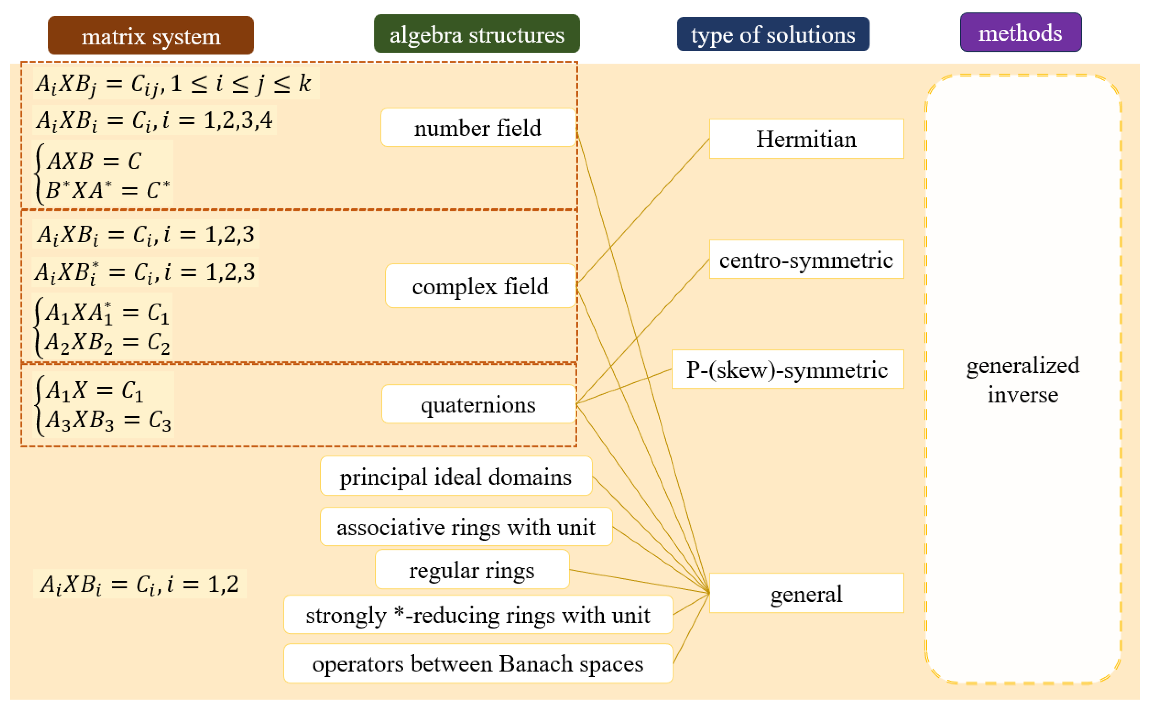
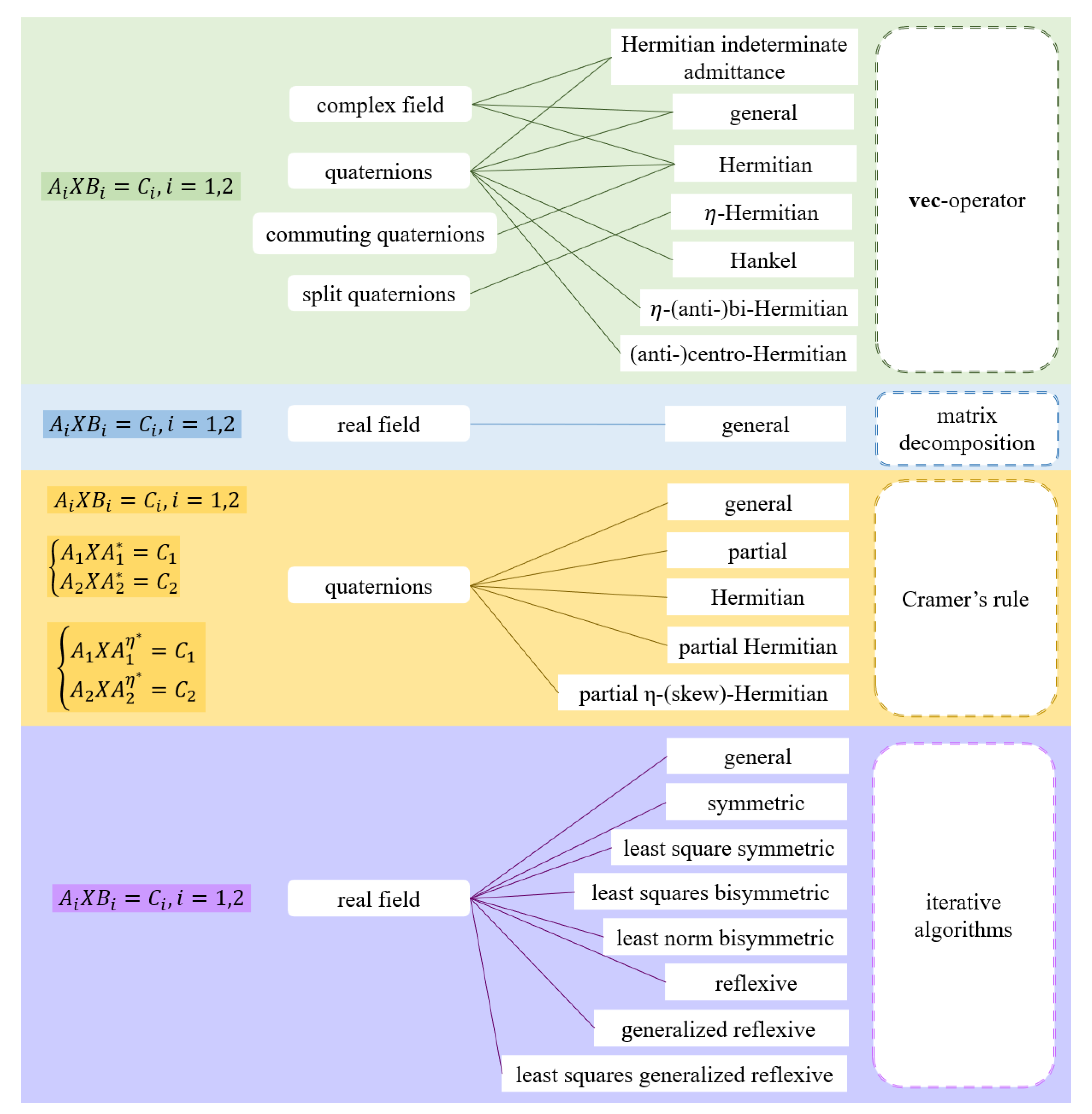

Table 1.
Definitions of some special matrices
| Symbols | Types of matrices | Definitions |
|---|---|---|
| symmetry real matrix | ||
| anti-symmetry real matrix | ||
| bi-symmetry real matrix | and | |
| anti-bi-symmetry real matrix | and | |
| real generalized reflection matrix | ||
| reflexive matrix | and | |
| anti-reflexive matrix | and | |
| generalized reflexive matrix | ||
| Hermitian complex matrix | ||
| Hermitian quaternion matrix | ||
| -Hermitian quaternion matrix | ||
| -anti-Hermitian quaternion matrix | ||
| -bi-Hermitian quaternion matrix | and | |
| -anti-bi-Hermitian quaternion matrix | and | |
| j-self conjugate quaternion matrix | ||
| anti-j-self conjugate quaternion matrix | ||
| centro-symmetric quaternion matrix | ||
| anti-centro-symmetric quaternion matrix | ||
| P- | P-centro-symmetric quaternion matrix | |
| P- | P-anti-centro-symmetric quaternion matrix | |
| centro-Hermitian quaternion matrix | ||
| anti-centro-Hermitian quaternion matrix |
Disclaimer/Publisher’s Note: The statements, opinions and data contained in all publications are solely those of the individual author(s) and contributor(s) and not of MDPI and/or the editor(s). MDPI and/or the editor(s) disclaim responsibility for any injury to people or property resulting from any ideas, methods, instructions or products referred to in the content. |
© 2025 by the authors. Licensee MDPI, Basel, Switzerland. This article is an open access article distributed under the terms and conditions of the Creative Commons Attribution (CC BY) license (http://creativecommons.org/licenses/by/4.0/).
Copyright: This open access article is published under a Creative Commons CC BY 4.0 license, which permit the free download, distribution, and reuse, provided that the author and preprint are cited in any reuse.


