
Submitted:
29 June 2025
Posted:
30 June 2025
You are already at the latest version
Abstract
The aim of this paper is to tailor the geometry and material parameters of a three-layer railway track model to achieve favorable properties for the circulation of high-speed trains at very high velocities. The three layers imply that the model should have three critical velocities for resonance. However, in many cases, some of these values are missing and must be replaced by pseudocritical values. Since no resonance occurs at pseudo-critical velocities, even in the absence of damping, deflections never reach infinity. By using optimization techniques, it is possible to adjust the parameters so that the increase in vibrations remains minimal and does not pose a real danger. In this way, circulation velocities could be extended beyond the critical value, thereby increasing network capacity and consequently improving the competitiveness of rail transport compared to other modes of transportation, contributing to decarbonization. The presented results are preliminary and require further analysis and validation. Several optimization techniques are implemented, leading to designs with already rather high pseudo-critical velocities. Further research will show how these theoretical findings can be utilized in practice.
Keywords:
integral transforms
; critical velocity
; pseudo-critical velocity
; false critical velocity
; instability of a moving mass
; transient vibrations
; analytical solution
; optimization
1. Introduction
The railway enables the circulation of railway vehicles in a safe and comfortable manner. Prioritizing rail transport over road transport represents an effective approach to combating climate change and reducing the carbon footprint. In line with this, it is necessary to increase the capacity of the railway network by raising circulation velocity without compromising passenger safety and comfort. To achieve this, an adequate transfer of solicitations to the ground must be ensured. Given the high demands that rolling stock imposes on the rail, one of the most challenging problems is identifying the most suitable technical solutions capable of supporting an increase in traffic velocity under standardized conditions without compromising passenger comfort or vehicle ride quality.
The maximum attainable circulation velocity in railway systems is often constrained by the so-called critical velocity, which, in the context of a moving force, represents the lowest velocity at which waves can propagate through the supporting track structure. This velocity arises from the dynamic interplay between all structural components and corresponds to a resonance condition. Experimental data indicate that this threshold has already been reached under real operating conditions [1].
To deepen our understanding of such dynamic behavior, further investigations are conducted within the well-established framework of moving load problems—a subject that continues to attract significant interest in transportation engineering. To enhance computational tractability and facilitate optimization and sensitivity analyses, many studies adopt simplified models. These simplifications can pertain to either the structure, the vehicle, or both, depending on the specific aspect under study. Besides exploring the effect of key parameters on dynamic response, major areas of interest include resonance-related critical velocities and frequencies, system instability, and the interaction between moving neighboring inertial bodies.
Common structural simplifications have led to layered models comprising beams, concentrated masses, and spring-damper elements. These configurations are favored for their simplicity and computational efficiency, finding widespread application in both research and practice. A survey of foundation modeling approaches is available in the classical work [2], while the discrete–continuous modeling debate is discussed in [3]. Rail tracks are frequently represented as Euler–Bernoulli infinite beams supported by continuous elastic foundations with one [4,5,6,7], two [8,9], or three layers [10,11]. Alternatively, the Euler–Bernoulli formulation may be replaced with a Timoshenko beam model to account for shear deformation and rotary inertia [12,13,14]. To accurately reflect the influence of sleeper spacing, models incorporating discrete supports are also used [15]. Despite their simplicity, such idealized models have successfully captured various phenomena in railway dynamics, as demonstrated in [16]. Comprehensive studies on vehicle–track interactions can be found in [17,18,19], further affirming the practical value of simplified modeling approaches. A taxonomy of layered models is proposed in [20], while their experimental validation is discussed in [21]. Naturally, the inclusion of additional layers improves the model’s ability to capture real-world behavior.
The feasibility of three-layer models in railway applications is evaluated in [10], and comparative features of one-, two-, and three-layer systems are reviewed in [22]. Research aimed at determining model parameters often builds upon the ballast pyramid concept [23,24] and the Saller hypothesis from 1932 [25]. A detailed treatment of the pyramid model—referred to as the "stress cone model"—is presented in [26], where it is used to derive vertical ballast stiffness and identify dynamically activated ballast mass. Refinements include overlapping cones between adjacent sleepers in both longitudinal [27] and lateral directions [10].
A number of studies concerning constant forces acting on an infinite structure exploit semianalytical methods. Fully analytical formulations are derived in [28,29]. The objectives of these two works are very similar, with some differences in the characterization of the Winkler–Pasternak foundation and critical damping. Both papers are also focused on critical velocity.
Advanced methods such as wavelet transforms are used in [30] to investigate moving forces on a double-beam system. The Adomian decomposition method is applied to handle nonlinearity in the viscoelastic connection between beams, with the model later adapted into a two-layer version [31] and extended to include nonlinear foundation behavior [32,33]. These studies directly derive steady-state solutions and compare their results with experimental observations.
Other works address the limitations of classical beam theories [34,35,36]. Large deformations are handled in [37]; initial conditions are accounted for in [38]; non-uniform motion is analyzed in [39]. Related problems include changes in foundation stiffness [40,41] or analyses concerned with non-classical ballasted tracks [42].
Further studies related to this paper focus on sleeper spacing [43,44] or critical zones [45], where more accurate mechanical descriptions of the track components are necessary, thus requiring numerical methods. When dealing with foundation models, more general formulations should be applied [46].
Recent studies focus on the instability of moving inertial objects. In the book chapter [47], vibrational stability of mechanical oscillators on continuous beam–foundation systems is analyzed using the D-decomposition method, comparing two models: one with a stabilizer directly connected to the car body, and another with interconnected primary suspensions. Instability of a moving bogie, with the possibility of occurring in the subcritical velocity range, is addressed in [48]. Further subjects related to instability are discussed in the book chapters [49,50]. In [51], the importance of material characterization is demonstrated through laboratory (physical and mechanical) tests and finite element modeling using four different rock materials as ballast, aiming to reduce the use of stone materials and promote an optimized, sustainable concept for new railway projects. The effects of ballast thickness on subgrade stresses are analyzed in terms of subgrade bearing capacity and permanent deformation of geotechnical materials.
In [52], localized waves in an Euler–Bernoulli beam on a nonlinear elastic foundation with nonlinear structural damping under the action of a moving force are studied. New approximation formulas describing both linear and nonlinear damping characteristics are derived. The Ritz method and perturbation techniques are employed for this purpose. It is demonstrated that the nonlinear contribution reduces displacement amplitudes compared to the linear foundation; however, it also lowers the critical velocity. Additionally, there is never true resonance—displacements remain finite even in the absence of damping.
Machine learning and numerical approaches are compared in [53] with the aim of evaluating track performance. In [54], a novel perspective is presented for improving performance and reliability through material optimization based on wheel–rail interactions under variable load and track conditions in a Y25 bogie. As this involves more detailed numerical studies, finite element analysis is implemented.
In this paper, the geometry and material parameters of a three-layer railway track model are tailored to achieve favorable properties for the circulation of high-speed trains at very high velocities. Specifically, cases where the lowest critical velocity is replaced by a pseudo-critical value are optimized so that the vibration increase around this pseudo-critical velocity is negligible, and the next resonance as well as the onset of instability are as distant as possible. All results are presented (semi)analytically with very high precision and in dimensionless parameters to cover a wide range of scenarios. Then, real data are assigned to the optimal cases.
The paper is organized in the following way. In Section 2, the model, involved parameters, and the governing equations are presented. In Section 3, the terminology used is introduced, and issues related to the number of resonances and the role of critical and pseudo-critical velocities, including their similarities and differences, are explained, followed by the motivation for this work. In Section 4, first, one case study is presented, followed by several methods and optimization techniques such as design of experiments, Monte Carlo analysis, parametric search, and simulated annealing. Optimized data are connected to real parameters and compared. The present paper is concluded by a discussion of the results obtained, their utility, and future challenges. After that, conclusions are drawn. The paper includes one Appendix where all numerical data are summarized for ease of comparison.
2. Governing Equations and Parameters
The three-layer railway track model is quite popular due to its simplicity, easy manipulability, computational efficiency, and good agreement with reality [10]. It is schematically presented in Figure 1 [11].
To facilitate the analytical steps of the solution, all parameters are introduced into the governing equations in their distributed and dimensionless forms. Exploiting the symmetry, the model represents a half-track of a single-line straight section.
The governing equations in dimensionless parameters and moving coordinates read as (more details can be found in [11]):
where
where and describe the Euler-Bernoulli beam on top of the model by its bending stiffness and mass per unit length. Further, is the sleeper spacing, and are masses of the sleeper (half) and ballast cone, , , and are the vertical stiffnesses of the rail pads, ballast cone, and foundation, and the shear stiffness of the ballast layer, respectively, where is usually defined as distributed, while the other values are discrete. The ballast cone theory according to [26], and refined in [27,10], is essential in the definition of the governing parameters. is the axial force and the vertical force acting on a moving mass that is traversing the model at constant velocity . Unknown displacement fields of the beam , the sleeper , and the ballast are functions of spatial coordinate and time . By switching to moving coordinates passes to and then to their dimensionless counterparts:
further
and other parameters in Equations (5) and (6) are masses ( and ), stiffnesses (, and ), damping ratios (, and ) and the axial force ratio (). To complete the list of symbols is the Dirac delta function, and derivatives are denoted by the symbol of the respective variable, preceded by a comma.
This means that a Winkler beam characterized by , and is selected as the reference beam. is inverse of its characteristic length, is the critical velocity of a moving force, and is therefore the velocity ratio. For identification of the moving mass instability, it is assumed that the mass is always in contact with the beam. Finally,
Considering the range of admissible parameters specified in detail in [11], it is possible to conclude that the admissible ranges of the leading parameters are approximately as follows:
Nevertheless, it is also necessary to point out that there are general trends such as enlarging sleeper spacing, the introduction of novel lightweight materials, and other cost-saving measures, which can obviously affect these ranges.
Admissible intervals in Equation (10) were obtained in the following way: first, geometrical data needed for the stress cone theory were assumed as:
All values except for are given in [m]. , and are ballast height, base sleeper width, and angle of the ballast cone, as exemplified in Figure 2, [10].
Further, and are the rail gauge and the sleeper effective length. For the calculations, is used as the most common value, and so does not have to be introduced. Then, by using the ranges from Equation (11), the dynamically activated ballast volume is within the range (0.065–0.7) m3, and the parameter related to the vertical stiffness ranges within (0.79–3.36) m (multiplication by the ballast Young´s modulus yields the correct base unit of N/m). According to [10,11], the range (40–160) kg is considered for , and the ballast density is taken within the range (1200–2600) kg/m3. Further, values within the range (20–5000) MN/m are considered for , and (50–400) MPa for the ballast Young’s modulus, .
There is an obvious connection between and , as well as between and , as they are both connected to the reference beam. Their ratios must be bounded by the values determined as:
In what follows, “+” and “–“ will be used to identify the upper and lower bounds, respectively.
Additionally, it will be demonstrated that graphical representation in logarithmic scale for and is more advantageous, as already used in [22,11]. For the analysis in this paper, the full range does not have to be covered; thus, the following representation is proposed:
Which, for the ratios from Equation (13), defines a range for the difference between the indexes and :
3. Methods
3.1. Terminology
This subsection clarifies the adopted terminology. The moving force problem is defined as a longitudinally homogeneous supporting structure being traversed by a constant force at constant velocity. In such a case, the transient part of the solution is not very important, and if a steady-state solution exists, it is rapidly attained.
In this context: the critical velocity (CV) designates a velocity fulfilling four conditions:
(i) it marks a true resonance, meaning that when the force moves at this velocity, deflections tend to infinity in the undamped case (i.e., the steady-state solution is never reached);
(ii) this velocity marks a local minimum of the generalized mode number of an equivalent finite beam;
(iii) there is a sudden jump to zero deflection at the active point (AP) at a velocity infinitesimally higher; and
(iv) the CV value separates regions of instability in regular cases.
On the other hand, the false critical velocity (FCV), which is also a true resonance, marks a local maximum of the generalized mode number of an equivalent finite beam and has no influence on instability regions or the specific value at the AP.
In the three-layer model—as the three layers indicate—three CVs are expected, which means five resonances in the moving force problem: three corresponding to CVs and two to FCVs. In a regular case, there are five vertical asymptotes to the instability lines, marking two full branches in the first two regions delimited by the critical velocities; after that, the final branch tends to zero moving mass for infinite velocity [22,11].
Nevertheless, there are several exceptional cases. In fact, the number of resonances can be 1, 3, or 5. When it is less than 5, some FCVs do not exist, and CVs are replaced by pseudo-critical velocities (PCVs). Additionally, some cases at the boundary of separation regions may lead to a model exhibiting only three resonances, meaning two CVs and one FCV, or one CV and one PCV.
As already mentioned, when CVs are missing, they are replaced by PCVs. A PCV marks a peak in vibrations, but not an infinite value. Since no resonance occurs, even in the absence of damping, deflections never reach infinity. Unlike CVs, FCVs are never replaced, but they can be absent.
Determination of resonances can be done semianalytically as described in [22], but high precision must be implemented. It is extremely important to perform such determinations in the absence of damping, which can unequivocally distinguish a vibration peak from a true resonance. Many methods used by other authors—such as the Green’s function method—require damping for numerical stability and are therefore unsuitable.
PCVs can be determined by parametric analyses. However, when the peak is hardly visible, the peak at the AP, the maximum, and the minimum over the whole beam are usually attained for different velocities, and thus its value is ambiguous. Numerical precision is also essential here. Even if the calculation must be done without damping, MATLAB can be used because the roots required for calculating the steady-state shape can be separated into those defining propagating and evanescent waves. Evanescent waves can be analyzed in the vicinity of the AP. For propagating waves, it is possible to establish an analytical envelope function that can unequivocally identify the maximum and minimum over the entire beam without enlarging the tested region around the AP.
Namely, as our interest lies in the initial region of , then when , there are two pairs of real roots and four complex roots symmetrically covering the four quadrants. Negligible damping can be introduced to correctly separate the real roots for the shape ahead of and behind AP. The four real roots define two harmonic waves with constant amplitude and zero phase. It is then possible to calculate the envelope function, which has clearly defined maximum and minimum values over the entire beam. It is then only necessary to check whether, in the vicinity of the AP, these values are exceeded due to evanescent waves. When , there is only one harmonic wave, so the amplitude is easily determined and an envelope function is unnecessary.
In the previous text, the term instability line was used. This relates to the instability of moving inertial objects. In such an analysis, the transient part of the solution is essential; without it, the problem of instability would remain hidden. Instability is not a resonance-type phenomenon; there is a velocity interval within which the object becomes unstable. At the extremities of this interval, the object remains stable, and instability is verified only within. This is characterized by an exponential increase in vibration amplitudes. Thus, although the steady-state solution usually exists and is finite, it is never reached.
Instability is determined by solving the roots of the characteristic equation. The roots always come in pairs, identifying the harmonic parts of the full solution. When this part grows exponentially, the roots are termed unstable. The instability line is traced in the ( – ) plane as a boundary between regions with a different number of unstable roots. In this paper, only one moving mass is considered. For this case, for a selected , it is possible to track real-valued frequencies until a real-valued equivalent stiffness (or flexibility) of the supporting structure is detected; then, is calculated from the characteristic equation. In this way, the analysis remains in the real domain, and the D-decomposition method used by other researchers can be avoided.
3.2. Determination of Number of Resonances and Pseudo-critical Velocities
Having the admissible range of dimensionless parameters, it is not easy to analytically indicate the regions corresponding to a particular number of resonances. Even though the base of the semianalytical solution is polynomial and all denominators are removed, the final degree is 16, and several roots are redundant. However, it is relatively easy to calculate the number of resonances semianalytically for a particular case using software with adaptable precision (e.g., Maple or Mathematica). MATLAB is not convenient in this context, as damping should not be included and high precision in root determination is required.
The number of resonances is always odd—1, 3, or 5—corresponding to 1, 2, or 3 critical velocities (CV) and 0, 1, or 2 false critical velocities (FCV), as explained in the previous section.
Four selected cases are shown as a demonstration in Figure 3. It was found convenient to select , and , or alternatively and to use the logarithmic scale for and , as indicated in Equation (14). This means that both indexes and were selected for the semianalytical determination from discrete values ranging from 1 to 101 in increments of 1.
As already mentioned, these graphs can only be obtained semianalytically using Maple or similar software because MATLAB does not provide sufficient accuracy in root determination, which is essential.
Once the number of expected resonances is known, the pseudo-critical velocity (PCV) must be determined, as it is often lower than the first resonance. In such cases, the PCV plays the role of a critical velocity for track design. Specifically, in cases with fewer than 5 resonances, when the PCV is lower than the first resonance, it is identified as the velocity that should not be exceeded. Hence, it can be termed the design critical velocity (DCV).
PCVs, which can be determined by parametric analysis, may be well-pronounced or ambiguous in the sense that the peaks do not always occur at the same position. The following figures explain these issues graphically. The case from Figure 3(d) is selected first. Then, in addition to , and () and , are used to identify cases with 1, 3, and 5 resonances..
In Figure 4, the case with 1 resonance is shown. This is an exceptional case characterized by a maximum of 3 resonances. Since only one resonance is present, the FCV is absent. The PCV is relatively well-pronounced at for both the maximum and minimum over the whole beam, while the peak at AP occurs at . These values are determined with a precision of 0.001, which corresponds to the step size used in the parametric analysis. Resonance occurs at .
In Figure 5, the case with 3 resonances is shown. Two CVs are clearly marked by a sudden jump to zero at the AP: and . Then, is the FCV. There is also a barely visible PCV with peaks at for the maximum and minimum over the whole beam, while the peak at AP occurs at . These values are determined with a precision of 0.0001, which is the step size used in the parametric analysis.
Finally, in Figure 6, the case with 5 resonances is shown. Three CVs are clearly marked by a sudden jump to zero at the AP: , and . Between them, two FCVs occur: and . There are no indications of other vibration peaks.
Due to the challenges in determining the PCV—first, the necessity of parametric analysis instead of semianalytical methods, and second, the ambiguity in identifying clear peaks—it is worthwhile to explore other possibilities. In Figure 5, at least, the maxima and minima over the beam occurred at the same , but this is not always the case. Therefore, the PCV can be ambiguous when the peaks do not coincide.
Since the PCV replaces the CV in separating instability regions, it is natural to propose that it should be predicted by , which indicates a vertical asymptote in the instability line. This newly proposed approach exploits the regularity of the single moving mass problem, exemplified in the one-layer model in Figure 7.
It is demonstrated in Figure 7 that, as the damping ratio decreases, the instability lines approach the CV. Therefore, a very good estimate of the CV can be obtained by identifying the onset of instability for infinitely low damping. Such calculations can be performed semianalytically in Maple or similar software because a high number of digits of precision is required. Infinitely low damping and infinitesimally small real-valued frequency are used to find an -value leading to a real-valued equivalent stiffness (or flexibility). The corresponding tends to infinity.
Applying the same reasoning to the three-layer model, it should be possible to identify the lowest PCV. This was tested for the case shown in Figure 3(a) with , and . In Figure 8(a), , and in Figure 8(b), . The latter case is the only one where the region of 3 resonances extends fully, and 5 resonances occur only at the very beginning.
It can be concluded from Figure 8 that PCV identification works well: the line of green crosses is smooth, as expected. In regions with 5 resonances, the crosses coincide, while in other regions, green crosses indicate a much lower value. Nevertheless, there are cases—as already mentioned—where the maximum number of resonances is only 3. Then, the crosses match in the region of 3 resonances, as shown in Figure 9, where the results of the parametric analysis are also included to show that no additional peaks occur (higher velocities are not shown but were tested). The graph in part (a) is plotted only up to for clarity.
In Figure 9(b), the resonances are: 0.339502; 0.377294 and 0.816655, corresponding to CV, FCV, and CV, respectively. The lowest asymptote is at , which perfectly matches the lowest resonance. This shows that the proposed technique works well in most cases. However, there are exceptions where the lowest PCV is lower than the lowest asymptote. These cases are, in fact, the focus of this paper.
This section concludes by illustrating the effect of PCV, CV, and FCV on instability lines in typical cases. When there are 5 resonances, three of them correspond to CVs and two to FCVs. Five vertical asymptotes to the instability lines then appear, defining two full branches in the first two regions delimited by the CVs. Beyond that, the final branch tends to zero as approaches infinity. When there are fewer resonances, CVs may be replaced by PCVs. In contrast, FCVs are never replaced and may be absent, as already mentioned.
The same cases as previously shown in [11] are selected for demonstration. These cases differ by , highlighting how this parameter affects the number of resonances. Specifically, both cases have , , and . For , there are 5 resonances (0.151–CV1; 0.152–FCV; 0.627–CV2; 0.851–FCV; 4.244–CV3). However, for , there is only one (~0.149–PCV1; 0.599–PCV2; 2.388–CV3). This is demonstrated in Figure 10.
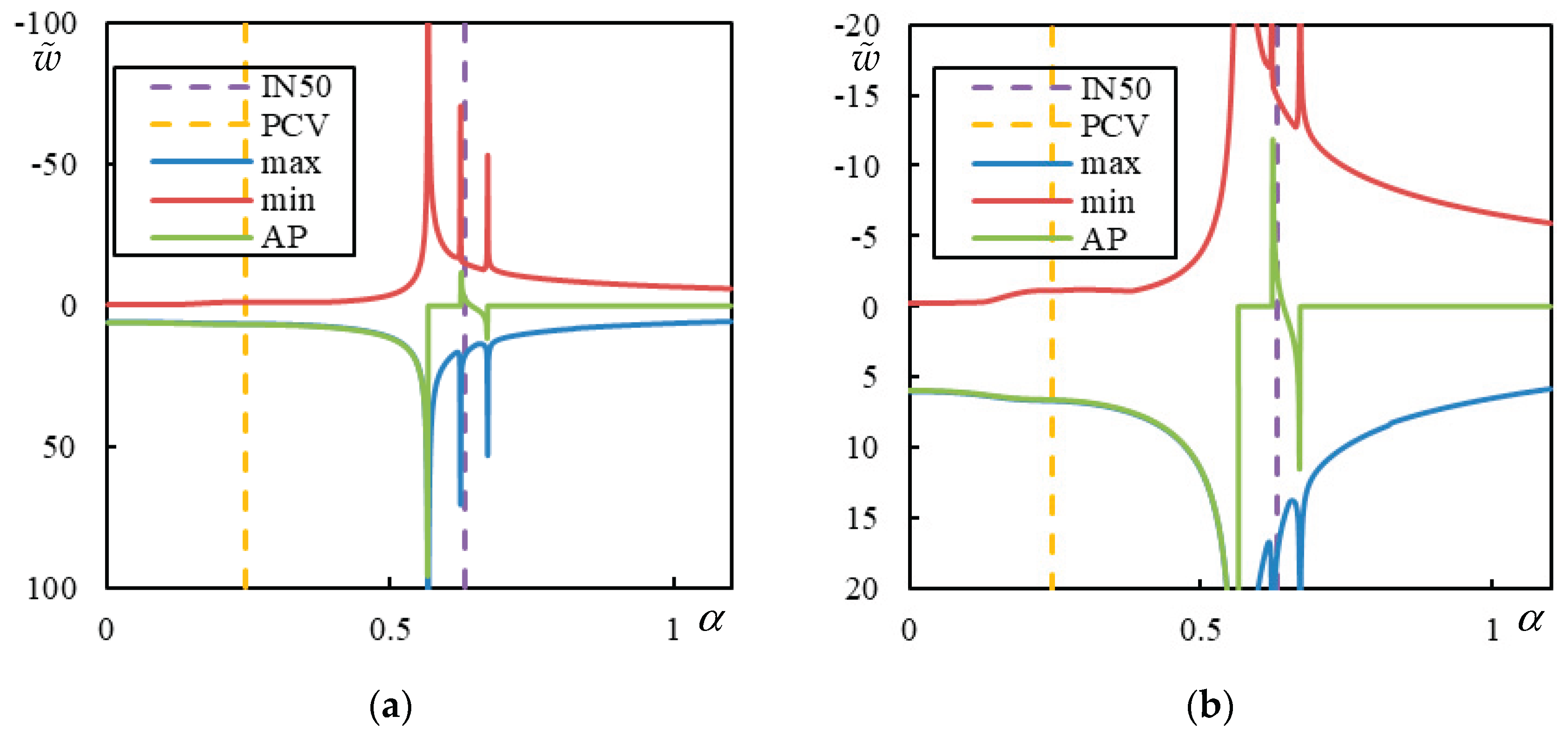
It is clear from Figure 10 that the FCV does not influence the separation of instability lines into three distinct regions. It is further shown that PCVs act as CVs, and with decreasing damping, instability lines approach either the CV or PCV. In the middle region, larger deviations are observed from the right than from the left. To complete this analysis, the corresponding real-valued frequency , which gives rise to Figure 10 as a root of the characteristic equation, is plotted in Figure 11.
Figure 11 again demonstrates that as damping decreases, CV and PCV are approached by vertical asymptotes for which tends to zero and tends to infinity. However, part (b) shows that in the first region, the damping level is not sufficiently low to clearly illustrate this behavior.
An interesting situation occurs when the above-described technique fails and such an asymptote does not exist. In these cases, only a slight increase in vibration is observed at the PCV. Alternatively, an asymptote may exist, but the instability line covers only unreasonably high values, so that instability cannot occur. In such cases, circulation velocities can exceed the expected critical velocity.
3.3. Motivation and Aim
As already mentioned, the motivation for this analysis lies in the observation that there are cases where the DCV is a PCV, which is not identified by a vertical asymptote. Thus, it appears possible to tailor the parameters in a way that reduces such vibrations, thereby extending the operational range into the supercritical region.
This suggests that it may be feasible to adjust the parameters of the model using optimization techniques so that the increase in vibrations remains minimal. Consequently, the DCV could be shifted to higher values without compromising safety—meaning, without the risk of excessive vibrations or potential instability. In more detail, the parameters must be adjusted such that the peak at the PCV is minimized, while simultaneously ensuring that the first resonance and the onset of instability for a reasonable value of and a moderate damping level occur at the highest possible velocity.
Mathematically, the first criterion is defined as the ratio between the highest upward displacement at the DCV = PCV, denoted , and the maximum downward displacement in the static case, . The reasoning is twofold: first, because dimensionless displacements are scaled with respect to the static displacement of a reference beam, it would not be reasonable to use unity for comparison; second, because upward displacements are more critical, they were chosen as the primary criterion.
This criterion is combined with two others: the lowest resonance , and the velocity at the onset of instability for a representative mass under 1% damping ratio at all levels, . Based on these, the performance index (PI) is defined as:
This PI also serves as the objective function, with the aim of finding its minimum within the admissible domain.
Several optimization methods were tested, beginning with statistical analyses—in particular, design of experiments (DOE) and response surface methodology—followed by parametric search (PS), the Monte Carlo method (MC), and Simulated Annealing (SA). It was also examined whether a full analysis was necessary or if some pre-selection could be applied. Certain parts required computation in Maple due to the need for increased numerical precision, while other parts could be handled in MATLAB.
4. Particular Case Analysis
4.1. Preliminary Tests
In this section, a particular case is tested to check the viability of the PI definition given by Equation (16). It is obvious that such cases must have a sufficiently large region of , where the difference between PCV and or is significant; otherwise, no improvement can be obtained. For this selection, the analysis of the number of resonances is useful, because these cases must have a reduced number of resonances. The selected case is characterized by , and . Two indexes are chosen to characterize , namely and . is tested for discrete values . Results are presented in Figure 12.
Several curves are plotted in Figure 12. In the legend: “peak” means at the first peak in upward displacement, identifying the lowest PCV determined by parametric analysis in MATLAB.
It can be concluded from Figure 12(b) that the PCV line is not realistic, because it should be smooth. Very accurate calculation is used by implementing function envelopes for the propagating part of the solution; thus, this decrease is not a numerical error but an indication of a premature peak, which should be disregarded for PCV determination. With regularization, the graph in Figure 13 is obtained.
From Figure 12 and Figure 13, it can be concluded that there is a sufficiently large region of , where the difference between PCV and or is quite large, confirming the feasibility of the adopted approach. Calculating PI for these cases, values of 1.3854 at and 0.5412 at are obtained for and , respectively.
However, it is not sufficient to calculate PI alone, because the feasibility of the data used must be confirmed. First, Equations (12) and (15) must be fulfilled. Unfortunately, this is still not sufficient.
4.2. Real Data Identification
As already mentioned, even when the feasibility of the main dimensionless parameters is confirmed by Equations (12) and (15), this does not ensure the existence of a corresponding real data set within the intervals from Equation (11), nor within other ranges for , , and , as indicated in Section 2 (text below Figure 2). It is also necessary to consider realistic values for ( or ) and , [11], which complete the full set of parameters defining the intervals indicated in Equation (10).
The selection of real parameters can be conveniently carried out in the following way. First, the stress cone is parameterized according to:
For each set of parameters, the dynamically activated ballast volume is calculated in [m3], and the parameter related to the ballast layer vertical stiffness is calculated in [m]. Knowing the optimal, i.e., target values , , and , it must hold:
Then, if these conditions are fulfilled, the selection may continue by defining admissible values:
Further:
Finally, if the interval has some intersection with , and also the interval has some intersection with , then feasible design values can be found. As only two rail profiles are commonly used, either 54 or 60 kg/m is selected. For each of these profiles is known. It was further confirmed during other optimization techniques that the optimal is usually very high; thus, in this procedure, it is more convenient to take the lowest feasible value. This completes the definition of the reference beam, and the missing values are simply calculated.
All results are summarized in tables, which are conveniently placed in the Appendix so that the results of all methods can be consulted together. In Table 1, the main optimized data are given in the form of optimized dimensionless parameters, PI, PCV, and an indication of possible extension, both by absolute -value and by percentage increase with respect to PCV. Table 2 summarizes the parameters of the stress cone; Table 3 lists the other values used to match the optimized data.
4.3. Design of Experiments and Response Surface
DOE and the response surface were the first optimization approaches used. Unfortunately, the response surface did not yield any improvement. When a larger design domain was applied, several cases with a set of fixed parameters , , and produced undefined PI across the full range of . Consequently, it was necessary to use a penalizing value, which distorted the response surface. Even on a more restricted design domain encompassing the particular case from Section 4.1, a reasonable estimate of already known values was never obtained. A Monte Carlo search over the response surface indicated the best choice at one of the factorial design points. Residues were not well-behaved, and thus this type of analysis had to be disregarded from further steps.
The best value obtained from this analysis, after removing non-feasible cases, was PI=0.4956, achieved for , , , and . In this case, the full factorial design was performed for , , , , , , , and , and the best feasible choice corresponded to the combination ++--. Results of this analysis are presented in Figure 14, which shows that PCV=DCV can be increased by 44.05%. Numerical values are included in Table 1 (Appendix).
In Figure 14, the yellow dashed line marks the first peak in upward displacement indication in this way PCV=DCV. The second criterium is governed by , which is not marked by a vertical line because it is identified through the properties of CV—that is, a sudden jump to zero displacement at AP. The corresponding probability plot is shown in Figure 15.
The best design obtained during DOE (line 1 in Table 1) offers many possibilities for selecting a corresponding set of real data. As it is not feasible to present all of them, only two representative cases are selected, and the corresponding values are provided in Table 2 and Table 3.
5. Optimization and Parametric Search
A full analysis, as reported in Figure 12 and Figure 13 and performed in DOE, is quite time-consuming and therefore not suitable for use in metaheuristic optimization methods or parametric search. Consequently, these methods were applied only to a preselection of favorable cases, after which the best case was further analyzed over . Preselection was implemented in two ways: based on cases with the highest differences in or in over the range of . can be easily extracted in MATLAB; however, lower damping levels would be prone to numerical errors due to MATLAB’s double precision. had to be calculated in Maple because high precision in root determination is required. In what follows, will be used for percentage difference in over the range of and for the percentage difference in .
5.1. Monte Carlo Method
MC method was performed with preselection of the most favorable cases according to . The design domain was defined as , , , , , , and .
It was not useful to repeat the analysis, because the MATLAB function rand tends to reuse the same randomization, and several tested cases were duplicated. The best value obtained was 88.89%, achieved for , , and . This case was then analyzed for PI. Results of the analysis over are presented in Figure 16. Asymptote and instability were only tested in the relevant region where PCV does not coincide with .
at minimum value of PI was gradually increased util at least one feasible design appeared. This happened for where PI=0.1905. Numerical data obtained are summarized in Table 1, Table 2 and Table 3. Final results are shown in Figure 17. is again decisive for PI, and the possible increase in DCV is 205.76%.
5.2. Parametric Search
PS was also performed using preselection of the most favorable cases. Both - and -based options were used. Results of this preselection are shown in Figure 18 and Figure 19.
After preselection, the four best cases were analyzed for PI over . at the minimum PI was gradually increased util at least one feasible design appeared. Final results are shown in Figure 20, Figure 21, Figure 22 and Figure 23. is again decisive for PI.
PI values in these four cases are 0.4257; 0.4115; 0.2517and 0.2462, leading to a possible increase in DCV of 55.60%; 65.64%; 132.22% and 182.10%, respectively. Numerical data are summarized in Table 1, Table 2 and Table 3.
5.3. Simulated Annealing
SA was selected as another metaheuristic optimization method due to its ease of implementation in MATLAB. The predefined parameters governing the optimization process were kept unchanged. The design domain was defined as , , , , , , , and , and used in this order. Several initial data sets were used for preselection according to , which was searched as a minimum.
Figure 24 shows the results of different runs.
The best value obtained is 1.46401, corresponding to 89.53%, which is better than that obtained by the MC method (88.89%) but worse than from the PS (89.90%). The preselected parameters , , , and were then used for detailed analysis of PI. As before, at the minimum value of PI was gradually increased until at least one feasible design appeared, which occurred for , for which PI=0.2055. The results of analysis over are presented in Figure 25. Asymptote and instability were again tested only in the relevant region where PCV does not coincide with .
Final results are shown in Figure 26. is again decisive. DCV=0.2437 could allow for an additional increase of 132.22%.
6. Discussion
In the previous sections, several feasible designs for which PI was evaluated as optimal have been presented. It is worthwhile to remark that was never decisive in these cases, and the extension of DCV was always guided by . From Table 1, it is evident that and exhibit higher dispersion, while and have very similar values in all cases. Finally, appears almost exclusively, except in the MC method—likely because a zero value was improbable to be selected randomly along with other optimal parameters. Furthermore, higher generally provides larger improvements, and is always much lower than .
at minimum value of PI was gradually increased util at least one feasible design appeared in all cases, except for DOE, where, in fact, no optimization was presented. Since these designs are the first to appear, this implies that some data will lie at the limit values of the considered ranges. As such, they might seem unrealistic, but it must be noted that further increase of can lead to better selections without significantly compromising the PI value. Generally, for higher , the possible increase up to is more favorable; however, the ratio is increasing.
Parametric searches with a base value of can naturally only identify designs where this is possible—meaning designs using wooden sleepers. Nevertheless, this option was not disregarded, because it is essential to consider the possibility of using novel lightweight materials in the future.
Some of the real data from Table 2 and Table 3 may seem unreasonable, but this results from the initial ranges of possible values.
Due to the consistency of results obtained by different approaches, exploring other methods would not be useful.
The results confirm that preselection is useful and reduces calculation time, but the connections are not straightforward. It is not necessarily true that the best preselection yields the best PI and, at the same time, the highest possible increase in DCV.
When using the lowest feasible , combinations with relatively high led to the appearance of the lowest found in the literature in all feasible data shown in Table 3. Similarly, for the same reason, is relatively high, resulting in quite high DCV—difficult to attain with current train designs. This implies that although the possible increase is large, it may be practically unimportant. Nevertheless, these results may inspire new approaches and provide guidance toward optimizing track design.
Further analyses are needed to verify whether PI was defined appropriately or if it should be modified. Since instability was never found to be decisive, it can likely be excluded from this analysis, allowing more detailed investigations.
Additional tests are also necessary because although several authors use this model without shear resistance, it must be verified whether such modeling is truly valid in practical applications.
7. Conclusions
In this paper, tailoring of input geometric and material data of the railway track was presented, with the objective of identifying cases where the first increase in vibrations is negligible and can therefore be bypassed.
Several optimization techniques and approaches were employed, leading to similar conclusions. However, the results require further examination in several aspects. In particular, the adequacy of the proposed PI must be evaluated. Since all results showed very high DCV with negligible increase in vibration, the significance of a further increase diminishes. It is thus necessary to investigate whether similar outcomes could be achieved for lower real velocities, where the potential for meaningful improvements is greater.
Results were obtained semianalytically with very high precision. This was crucial for accurately determining the number of resonances and identifying the first peak in upward vibration.
It was found that DCV can be significantly increased by optimizing the design parameters. However, such cases almost exclusively result in designs where the DCV is already very high. Therefore, the practical significance of further increase becomes questionable, as already mentioned above.
In all cases, very soft rail pads emerged in the final optimized design. It is essential to verify whether such configurations are feasible. Thus, the results suggest a tendency toward:
- Very high foundation stiffness,
- Low rail pad stiffness,
- Zero ballast shear stiffness.
Further research is particularly needed regarding ballast shear stiffness. In actual designs, eliminating it entirely may not be realistic. While it might be reduced via rail pretension, such an approach is not practical.
Due to the scope of this study, these aspects will be addressed in future research. It is believed that the theoretical findings presented here can contribute to the development of optimal track designs incorporating novel materials. Their implementation in real-world designs remains a subject for further investigation.
Supplementary Materials
There is no supporting material as all results are presented in the paper.
Author Contributions
not applicable-sole author.
Funding
The author acknowledges Fundação para a Ciência e a Tecnologia (FCT) for its financial support via the project LAETA Base Funding (DOI: 10.54499/UIDB/50022/2020). EEA grant FBR_OC2_45: SMART - Sustainable Maintenance and Rehabilitation of Railway Track is also acknowledged.
Data Availability Statement
All data are contained in the paper.
Acknowledgments
The author acknowledges Fundação para a Ciência e a Tecnologia (FCT) for its financial support via the project LAETA Base Funding (DOI: 10.54499/UIDB/50022/2020). EEA grant FBR_OC2_45: SMART - Sustainable Maintenance and Rehabilitation of Railway Track is also acknowledged.
Conflicts of Interest
The author declares no conflicts of interest. The funders had no role in the design of the study; in the collection, analyses, or interpretation of data; in the writing of the manuscript; or in the decision to publish the results.
Abbreviations
The following abbreviations are used in this manuscript:
| AP | Active point (force position) |
| CV | Critical velocity |
| DCV | Design critical velocity |
| DOE | Design of experiments |
| FCV | False critical velocity |
| MC | Monte Carlo method |
| PCV | Pseudo-critical velocity |
| PI | Performance index |
| PS | Parametric search |
| SA | Simulated annealing |
Appendix A
This Appendix summarizes the data obtained by optimization, they are mentioned in Section 4 and Section 5.

Table A1.
Summary of the best solutions obtained in each method.
| Type | PI | PCV | % | ||||||
|---|---|---|---|---|---|---|---|---|---|
| DOE | 4 | 12 | 16 | 40 | 0 | 0.4956 | 0.4456 | 0.6419 | 44.05 |
| MC ( ) | 5.5244 | 44.1292 | 20 | 44.8870 | 0.1111 | 0.7163 | 0.2326 | 0.7112 | 205.76 |
| PS1 ( ) | 1 | 16 | 17 | 49 | 0 | 0.4410 | 0.4257 | 0.6624 | 55.60 |
| PS2 ( ) | 1 | 16 | 18 | 50 | 0 | 0.4505 | 0.4115 | 0.6816 | 65.64 |
| PS3 ( ) | 3.5 | 42 | 13 | 40 | 0 | 0.2159 | 0.2517 | 0.5845 | 132.22 |
| PS4 ( ) | 3.5 | 42 | 19 | 46 | 0 | 0.3355 | 0.2462 | 0.6945 | 182.10 |
| SA ( ) | 5.3333 | 42.8571 | 12 | 47.3333 | 0 | 0.2055 | 0.2437 | 0.5660 | 132.22 |
In Table A1 the following designation is used: DOE (design of experiments); MC (Monte Carlo), PS (Parametric Search) and SA (Simulated Annealing) with indication in brackets of the preselection used.
Table A2.
Summary of the feasible data of the stress cone obtained in each method.
| Type | [m] | [m] | [º] | [m] | [m3] | [m] |
|---|---|---|---|---|---|---|
| DOE | 0.6 | 0.3 | 50 | 0.36 | 0.2231 | 2.3821 |
| DOE | 0.6 | 0.35 | 25 | 0.2 | 0.1510 | 1.089 |
| MC ( ) | 0.5 | 0.6 | 50 | 0.34 | 0.4592 | 1.2568 |
| PS1 ( ) | 0.8 | 0.3 | 50 | 0.36 | 0.2682 | 2.6634 |
| PS2 ( ) | 0.8 | 0.3 | 50 | 0.36 | 0.2682 | 2.6634 |
| PS3 ( ) | 0.7 | 0.6 | 50 | 0.3 | 0.6128 | 1.5289 |
| PS4 ( ) | 0.7 | 0.6 | 50 | 0.3 | 0.6128 | 1.5289 |
| SA ( ) | 0.5 | 0.6 | 50 | 0.32 | 0.4577 | 1.2442 |
Table A3.
Summary of the other data to match the optimized parameters ( indicates the velocity at resonance).
Table A3.
Summary of the other data to match the optimized parameters ( indicates the velocity at resonance).
| Type | [kg/m] | [kg] | [kg/m3] | [MN/m2] | [MN/m] | [MPa] | DCV[m/s] | [m/s] |
| DOE | 60 | 144 | 1937 | 198 | 20 | 177 | 449 | 646 |
| DOE | 54 | 130 | 2575 | 198 | 20 | 388 | 473 | 681 |
| MC ( ) | 54 | 149 | 2594 | 150 | 20 | 372 | 230 | 704 |
| PS1 ( ) | 54 | 43.2 | 2577 | 132 | 20 | 399 | 408 | 636 |
| PS2 ( ) | 54 | 43.2 | 2577 | 118 | 20 | 399 | 384 | 636 |
| PS3 ( ) | 54 | 132.3 | 2591 | 239 | 20 | 390 | 280 | 651 |
| PS4 ( ) | 54 | 132.3 | 2591 | 120 | 20 | 390 | 231 | 651 |
| SA ( ) | 54 | 144 | 2528 | 376 | 20 | 396 | 304 | 705 |
References
- Madshus, C.; Kaynia, A.M. High-speed railway lines on soft ground: dynamic behaviour at critical train speed. J. Sound Vib. 2000, 231, 689–701. [Google Scholar] [CrossRef]
- Kerr, A. Elastic and viscoelastic foundation models. J. Appl. Mech. 1994, 31, 491–498. [Google Scholar] [CrossRef]
- Szolc, T. On discrete-continuous modelling of the railway bogie and the track for the medium frequency dynamic analysis. Engineering Transactions 2000, 48, 153–198. [Google Scholar] [CrossRef]
- Metrikine, A.V.; Dieterman, H.A. Instability of vibrations of a mass moving uniformly along an axially compressed beam on a viscoelastic foundation. J. Sound Vib. 1997, 201, 567–576. [Google Scholar] [CrossRef]
- Duffy, D.G. The response of an infinite railroad track to a moving, vibrating mass. J. Appl. Mech. 1990, 57, 66–73. [Google Scholar] [CrossRef]
- Stojanović, V.; Kozić, P.; Petković, M.D. Dynamic instability and critical velocity of a mass moving uniformly along a stabilized infinity beam. Int. J. Solids Struct. 2017, 108, 164–174. [Google Scholar] [CrossRef]
- Dimitrovová, Z. Dynamic interaction and instability of two moving proximate masses on a beam on a Pasternak viscoelastic foundation. Appl. Math. Modell. 2021, 100, 192–217. [Google Scholar] [CrossRef]
- Dimitrovová, Z. Two-layer model of the railway track: analysis of the critical velocity and instability of two moving proximate masses. Int. J. Mech. Sci. 2022, 217, 107042. [Google Scholar] [CrossRef]
- Dimitrovová, Z. Instability of vibrations of mass(es) moving uniformly on a two-layer track model: Parameters leading to irregular cases and associated implications for railway design. Appl. Sci. 2023, 13, 12356. [Google Scholar] [CrossRef]
- Rodrigues, A.F.S.; Dimitrovová, Z. Applicability of a Three-Layer Model for the Dynamic Analysis of Ballasted Railway Tracks. Vibration 2021, 4, 151–174. [Google Scholar] [CrossRef]
- Dimitrovová, Z.; Mazilu, T. Semi-Analytical Approach and Green’s Function Method: A Comparison in the Analysis of the Interaction of a Moving Mass on an Infinite Beam on a Three-Layer Viscoelastic Foundation at the Stability Limit—The Effect of Damping of Foundation Materials. Materials 2024, 17, 279. [Google Scholar] [CrossRef] [PubMed]
- Mazilu, T.; Dumitriu, M.; Tudorache, C. Instability of an oscillator moving along a Timoshenko beam on viscoelastic foundation. Nonlinear Dyn. 2012, 67, 1273–1293. [Google Scholar] [CrossRef]
- Verichev, S.N.; Metrikine, A.V. Instability of a bogie moving on a flexibly supported Timoshenko beam. J. Sound Vib. 2002, 253, 653–668. [Google Scholar] [CrossRef]
- Yang, C.J.; Xu, Y.; Zhu, W.D.; Fan, W.; Zhang, W.H.; Mei, G.M. A three-dimensional modal theory-based Timoshenko finite length beam model for train-track dynamic analysis. J. Sound Vib. 2020, 479, 115363. [Google Scholar] [CrossRef]
- Abea, K.; Chidaa, Y.; Quinay, P.E.B. , Koroa, K. Dynamic instability of a wheel moving on a discretely supported infinite rail. J. Sound Vib. 2014, 333, 3413–3427. [Google Scholar] [CrossRef]
- Mazilu, T. Interaction between a moving two-mass oscillator and an infinite homogeneous structure: Green’s functions method. Arch. Appl. Mech. 2010, 80, 909–927. [Google Scholar] [CrossRef]
- Nelson, H.D.; Conover, R.A. Dynamic stability of a beam carrying moving masses. J. Appl. Mech. Trans. ASME 1971, 38, 1003–1006. [Google Scholar] [CrossRef]
- Benedetti, G.A. Dynamic stability of a beam loaded by a sequence of moving mass particles. J. Appl. Mech. Trans. ASME 1974, 41, 1069–1071. [Google Scholar] [CrossRef]
- Mackertich, S. Dynamic response of a supported beam to oscillatory moving masses. J. Vib. Control 2003, 9, 1083–1091. [Google Scholar] [CrossRef]
- Knothe, K.L.; Grassie, S.L. Modelling of railway track and vehicle-track interaction at high frequencies. Veh. Syst. Dyn. 1993, 22, 209–262. [Google Scholar] [CrossRef]
- Grassie, S.L.; Gregory, R.W.; Harrison, D.; Johnson, K.L. The dynamic response of railway track to high frequency vertical excitation. J. Mech. Eng. Sci. 1982, 24, 77–90. [Google Scholar] [CrossRef]
- Dimitrovová, Z. On the critical velocity of moving force and instability of moving mass in layered railway track models by semianalytical approaches. Vibration 2023, 6, 113–146. [Google Scholar] [CrossRef]
- Ahlbeck, D.R.; Meacham, H.C.; Prause, R.H. The development of analytical models for railroad track dynamics. In Symposium on Railroad Track Mechanics; 1975. [CrossRef]
- Doyle, N.F. Railway Track Design: A Review of Current Practice. Bureau of Transport Economics (bte), 1980. Available online: https://www.bitre.gov.au/sites/default/files/op_035.pdf (accessed on 28/6/2025).
- Kerr, D. On the determination of the rail support modulus k. Int. J. Solids Struct. 2000, 37, 4335–4351. [Google Scholar] [CrossRef]
- Zhai, W.M.; Sun, X. A detailed model for investigating vertical interaction between railway vehicle and track. Veh. Syst. Dyn. 1994, 23, 603–615. [Google Scholar] [CrossRef]
- Zhai, W.M.; Wang, K.Y.; Lin, J.H. Modelling and experiment of railway ballast vibrations. J. Sound Vib. 2004, 270, 673–683. [Google Scholar] [CrossRef]
- Basu, D.; Kameswara Rao, N.S.V. Analytical solutions for Euler-Bernoulli beam on visco-elastic foundation subjected to moving load. Int. J. Numer. Anal. Methods Geomech. 2013, 37, 945–960. [Google Scholar] [CrossRef]
- Froio, D.; Rizzi, E.; Simões, F.M.F.; Da Costa, A.P. Universal analytical solution of the steady-state response of an infinite beam on a Pasternak elastic foundation under moving load. Int. J. Solids Struct. 2018, 132–133, 245–263. [Google Scholar] [CrossRef]
- Koziol, P. Wavelet approximation of the Adomian’s decomposition applied to a nonlinear problem of a double-beam response subject to a series of moving loads. J. Theor. Appl. Mech. 2014, 52, 687–697. [Google Scholar]
- Czyczula, W.; Koziol, P.; Kudla, D.; Lisowski, S. Analytical evaluation of track response in the vertical direction due to a moving load. J. Vib. Control 2017, 23, 2989–3006. [Google Scholar] [CrossRef]
- Koziol, P.; Pilecki, R. Semi-analytical modelling of multilayer continuous systems nonlinear dynamics. Arch. Civ. Eng. 2020, 66, 165–178. [Google Scholar] [CrossRef]
- Koziol, P.; Pilecki, R. Nonlinear double-beam system dynamics. Arch. Civ. Eng. 2021, 67, 337–353. [Google Scholar] [CrossRef]
- Kiani, K.; Nikkhoo, A. On the limitations of linear beams for the problems of moving mass-beam interaction using a meshfree method. Acta Mech. Sin. 2011, 28, 164–179. [Google Scholar] [CrossRef]
- Kiani, K.; Nikkhoo, A.; Mehri, B. Prediction capabilities of classical and shear deformable beam models excited by a moving mass. J. Sound Vib. 2009, 320, 632–648. [Google Scholar] [CrossRef]
- Kiani, K.; Nikkhoo, A.; Mehri, B. Assessing dynamic response of multispan viscoelastic thin beams under a moving mass via generalized moving least square method. Acta Mech. Sin. 2010, 26, 721–733. [Google Scholar] [CrossRef]
- Jahangiri, A.; Attari, N.K.A.; Nikkhoo, A.; Waezi, Z. Nonlinear dynamic response of an Euler–Bernoulli beam under a moving mass–spring with large oscillations. Arch. Appl. Mech. 2020, 90, 1135–1156. [Google Scholar] [CrossRef]
- Dimitrovová, Z. Complete semi-analytical solution for a uniformly moving mass on a beam on a two-parameter visco-elastic foundation with non-homogeneous initial conditions. Int. J. Mech. Sci. 2018, 144, 283–311. [Google Scholar] [CrossRef]
- Tran, M.T.; Ang, K.K.; Luong, V.H. Vertical dynamic response of non-uniform motion of high-speed rails. J. Sound Vib. 2014, 333, 5427–5442. [Google Scholar] [CrossRef]
- Fărăgău, A.B.; Metrikine, A.V.; van Dalen, K.N. Transition radiation in a piecewise-linear and infinite one-dimensional structure–a Laplace transform method. Nonlinear Dyn. 2019, 98, 2435–2461. [Google Scholar] [CrossRef]
- Fărăgău, A.B.; Keijdener, C.; de Oliveira Barbosa, J.M.; Metrikine, A.V.; van Dalen, K.N. Transition radiation in a nonlinear and infinite one-dimensional structure: A comparison of solution methods. Nonlinear Dyn. 2021, 103, 1365–1391. [Google Scholar] [CrossRef]
- Dai, J.; Lim, J.G.Y.; Ang, K.K. Dynamic response analysis of high-speed maglev-guideway system. J. Vib. Eng. Technol. 2023, 11, 2647–2658. [Google Scholar] [CrossRef]
- Ortega, R.S.; Pombo, J.; Ricci, S.; Miranda, M. The importance of sleepers spacing in railways. Constr. Build. Mater. 2021, 300, 124326. [Google Scholar] [CrossRef]
- Sañudo, R.; Miranda, M.; Alonso, B.; Markine, V. Sleepers spacing analysis in railway track infrastructure. Infrastructures. 2022, 7, 83. [Google Scholar] [CrossRef]
- Punetha, P.; Nimbalkar, S. Numerical investigation on dynamic behaviour of critical zones in railway tracks under moving train loads. Transp. Geotech. 2023, 41, 101009. [Google Scholar] [CrossRef]
- Dimitrovová, Z. Semi-analytical analysis of vibrations induced by a mass traversing a beam supported by a finite depth foundation with simplified shear resistance. Meccanica 2020, 55, 2353–2389. [Google Scholar] [CrossRef]
- Stojanović, V.; Deng, J.; Petković, M.D.; Ristić, M.A. Vibrational instability in a complex moving object: innovative approaches to elastically damped connections between car body components and supports. Modeling of Complex Dynamic Systems (Fundamentals and Applications) 2025, ch. 9, 197-233. [CrossRef]
- Dimitrovová, Z. Instability of a Moving Bogie: Analysis of Vibrations and Possibility of Instability in Subcritical Velocity Range. Vibration 2025, 8(2), 13. [Google Scholar] [CrossRef]
- Stojanović, V.; Deng, J.; Petković, M.D.; Ristić, M.A. Stability of vibrations of a system of discrete oscillators that are moving at an overcritical velocity. Modeling of Complex Dynamic Systems (Fundamentals and Applications) 2025, ch. 5, 81-105. [CrossRef]
- Stojanović, V.; Deng, J.; Petković, M.D.; Ristić, M.A. Modeling of a three part viscoelastic foundation and its effect on dynamic stability. Modeling of Complex Dynamic Systems (Fundamentals and Applications) 2025, ch. 8, 173-196. [CrossRef]
- Rosa, A.F.; Dias, S.C.; Brito, W.S.; Costa, R.C.; Moura, E.; Bernucci, L.L.B.; Motta, R.S. Laboratory and numerical analysis for enhanced ballast performance: towards sustainable railway track pavement design. Transportes 2025, 33, e3028. [Google Scholar] [CrossRef]
- Abramian, A.K.; Vakulenko, S.A.; Horssen, W.T.v. On the existence and approximation of localized waves in a damped Euler–Bernoulli beam on a nonlinear elastic foundation. Nonlinear Dyn. 2025. [CrossRef]
- Kazemzadeh, M.; Zad, A.; Yazdi, M. Railway Track Performance Over Geogrid-Encased Stone Columns Under High-Speed Train Loads: A Numerical and Machine Learning Approach. Transp. Infrastruct. Geotech 2025, 12, 175. [Google Scholar] [CrossRef]
- Baykara, C. Investigation of mechanical strength and deformation properties of Y25 bogie suspension systems by finite element analysis. Railway Sciences 2025. [CrossRef]
Figure 1.
The three-layer model of the railway track traversed by a moving mass, [11].
Figure 1.
The three-layer model of the railway track traversed by a moving mass, [11].
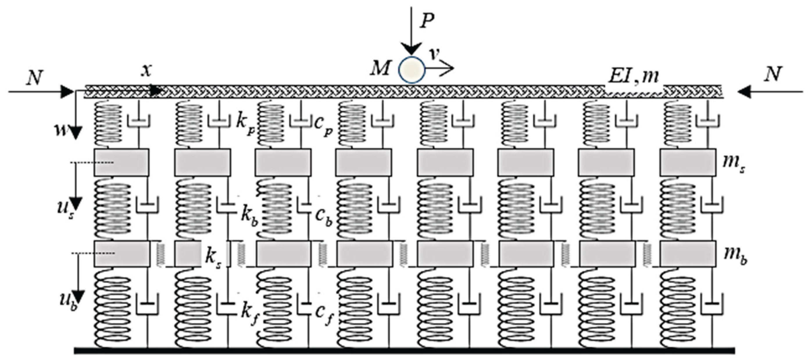
Figure 2.
Parameters related to stress cone theory.
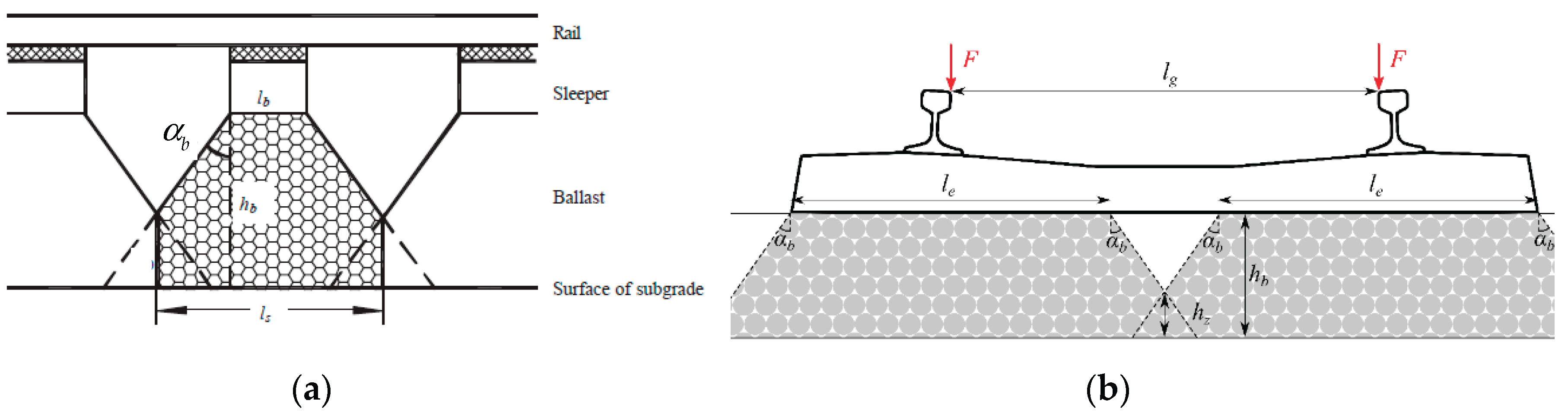
Figure 3.
Number of resonances in selected cases (1 – red, 3 – yellow, 5 – green): (a) , , ; (b) , , ; (c) , , ; (d) , , .
Figure 3.
Number of resonances in selected cases (1 – red, 3 – yellow, 5 – green): (a) , , ; (b) , , ; (c) , , ; (d) , , .
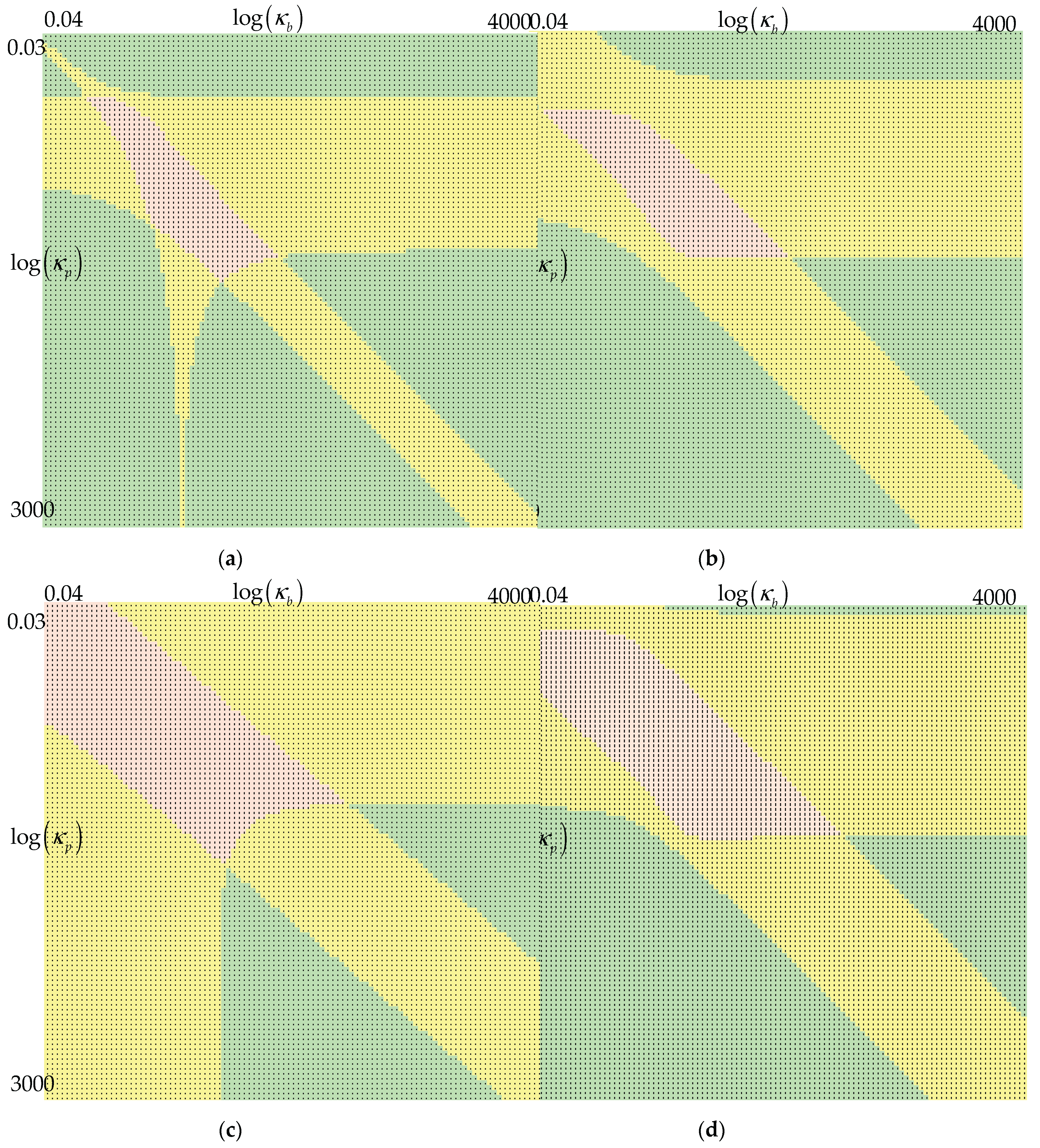
Figure 4.
Parametric analysis (AP – green, Maximum – blue, Minimum – orange displacement over the entire beam): , , , and
Figure 4.
Parametric analysis (AP – green, Maximum – blue, Minimum – orange displacement over the entire beam): , , , and

Figure 5.
Parametric analysis (AP – green, Maximum – blue, Minimum – orange displacement over the entire beam): , , , and Parts (a) and (b) refer to different -scale.
Figure 5.
Parametric analysis (AP – green, Maximum – blue, Minimum – orange displacement over the entire beam): , , , and Parts (a) and (b) refer to different -scale.
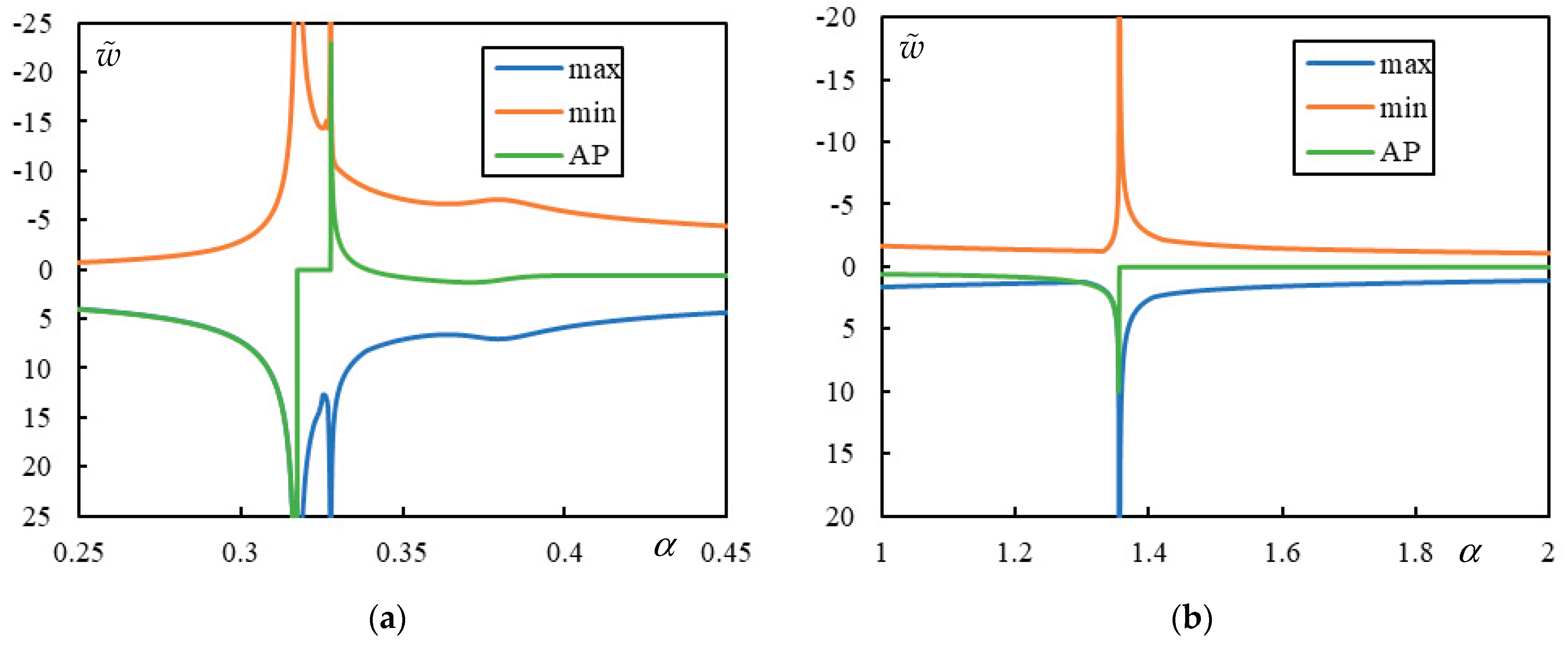
Figure 6.
Parametric analysis (AP – green, Maximum – blue, Minimum – orange displacement over the entire beam): , , , and Parts (a) and (b) refer to different -scale.
Figure 6.
Parametric analysis (AP – green, Maximum – blue, Minimum – orange displacement over the entire beam): , , , and Parts (a) and (b) refer to different -scale.
Figure 7.
Single moving mass problem on the one-layer model. Numbers in the legend represent the damping ratio. The dotted line marks the CV at .
Figure 7.
Single moving mass problem on the one-layer model. Numbers in the legend represent the damping ratio. The dotted line marks the CV at .
Figure 8.
Determination of the lowest PCV in the three-layer model. , and : (a) ; (b) . Orange crosses designate the lowest resonance; green crosses mark the lowest asymptote. Vertical orange lines separate regions based on the number of resonances.
Figure 8.
Determination of the lowest PCV in the three-layer model. , and : (a) ; (b) . Orange crosses designate the lowest resonance; green crosses mark the lowest asymptote. Vertical orange lines separate regions based on the number of resonances.
Figure 9.
Determination of the lowest PCV in the three-layer model. , and : (a) ; (b) the corresponding parametric analysis for . Orange crosses designate the lowest resonance; green crosses mark the lowest asymptote. Vertical orange lines separate regions based on the number of resonances.
Figure 9.
Determination of the lowest PCV in the three-layer model. , and : (a) ; (b) the corresponding parametric analysis for . Orange crosses designate the lowest resonance; green crosses mark the lowest asymptote. Vertical orange lines separate regions based on the number of resonances.
Figure 10.
Instability lines for , , and . (a) ; (b) . Dasher and dotted lines represent CV, FCV and PCV. Solid lines in different colors indicate different damping levels for .
Figure 10.
Instability lines for , , and . (a) ; (b) . Dasher and dotted lines represent CV, FCV and PCV. Solid lines in different colors indicate different damping levels for .
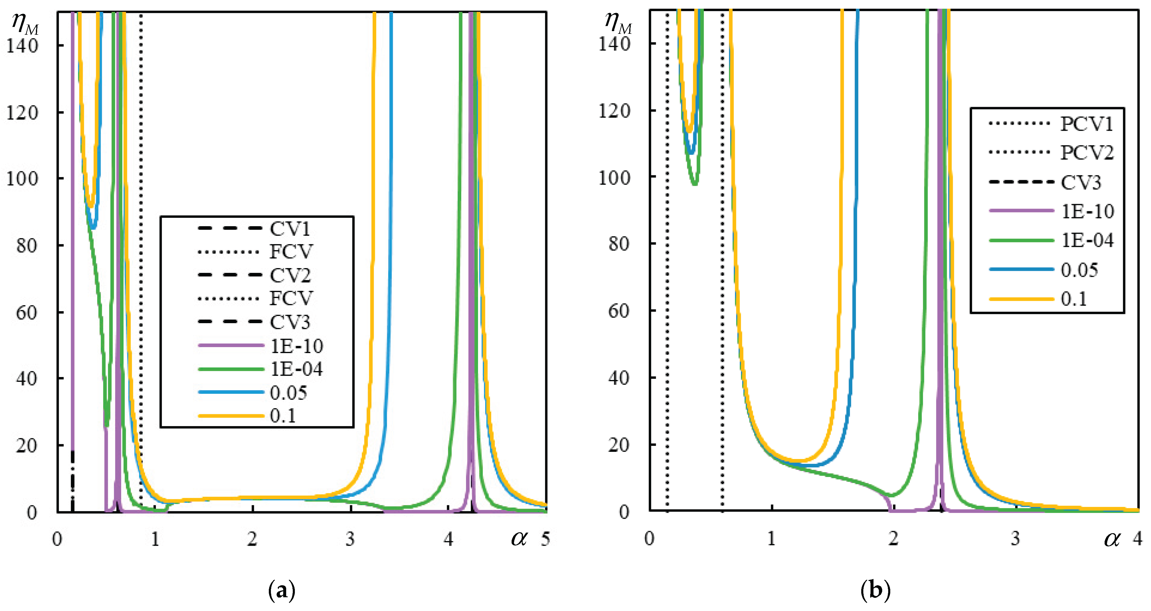
Figure 11.
Real-valued frequency for , , and . (a) ; (b) . Dasher and dotted lines represent CV, FCV and PCV. Solid lines in different colors indicate different damping levels for .
Figure 11.
Real-valued frequency for , , and . (a) ; (b) . Dasher and dotted lines represent CV, FCV and PCV. Solid lines in different colors indicate different damping levels for .
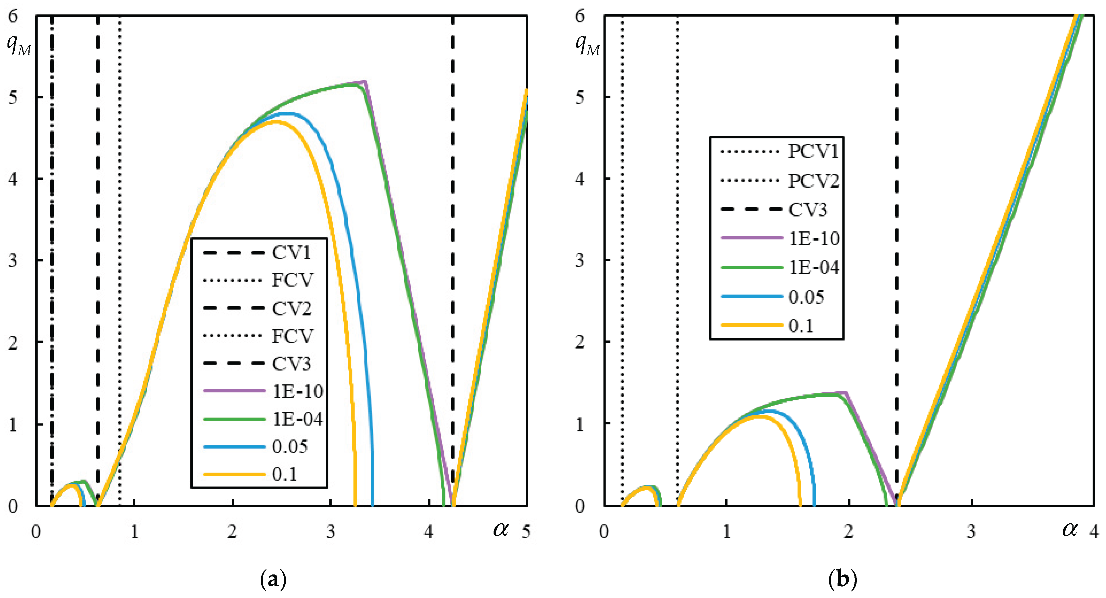
Figure 12.
Analysis related to determination of PI for , and . (a) ; (b) . In the legend: “peak” (violet) is PCV; “resonance” (red) is ; “asymptote” is at the lowest asymptote to instability lines (blue – negligible damping ; orange – 1% damping ); “alpha50” is .
Figure 12.
Analysis related to determination of PI for , and . (a) ; (b) . In the legend: “peak” (violet) is PCV; “resonance” (red) is ; “asymptote” is at the lowest asymptote to instability lines (blue – negligible damping ; orange – 1% damping ); “alpha50” is .
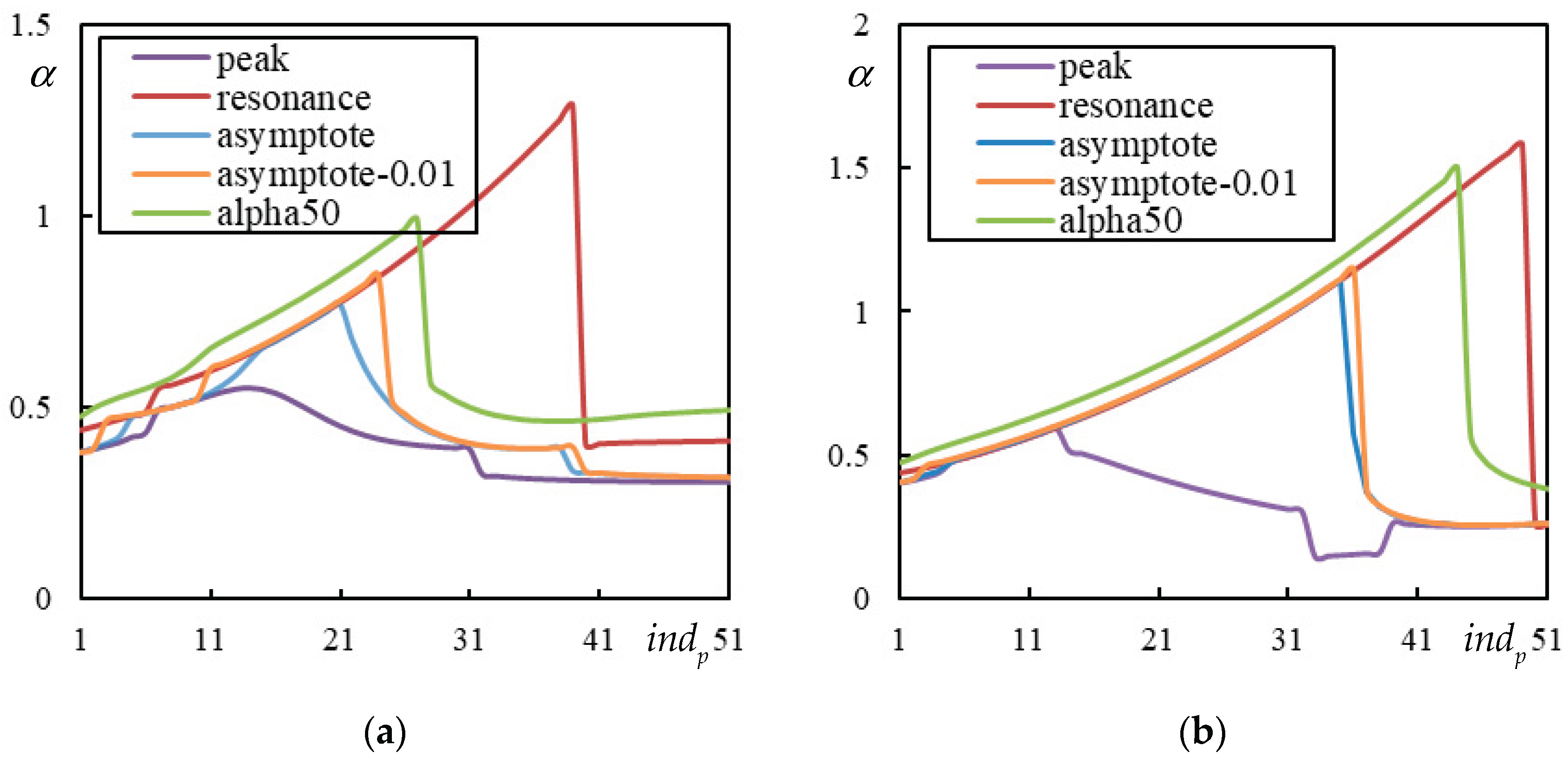
Figure 13.
Analysis related to determination of PI for , , and . In the legend: “peak” (violet) is regularized PCV; “resonance” (red) is ; “asymptote” is at the lowest asymptote to instability lines (blue – negligible damping ; orange – 1% damping ); “alpha50” is .
Figure 13.
Analysis related to determination of PI for , , and . In the legend: “peak” (violet) is regularized PCV; “resonance” (red) is ; “asymptote” is at the lowest asymptote to instability lines (blue – negligible damping ; orange – 1% damping ); “alpha50” is .
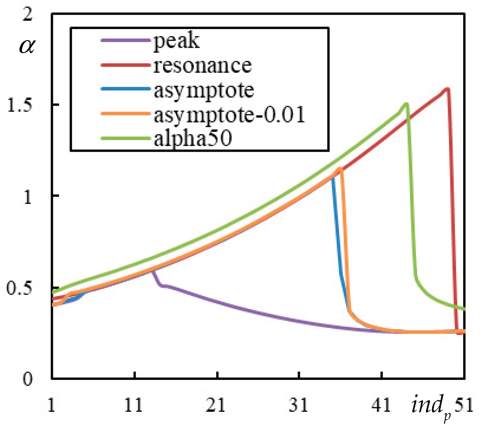
Figure 14.
Parametric analysis (AP – green, Maximum – blue, Minimum – red displacement over the entire beam): , , , and . Parts (a) and (b) refer to different -scale. PCV is marked by an orange dashed line and by a violet dashed line.
Figure 14.
Parametric analysis (AP – green, Maximum – blue, Minimum – red displacement over the entire beam): , , , and . Parts (a) and (b) refer to different -scale. PCV is marked by an orange dashed line and by a violet dashed line.
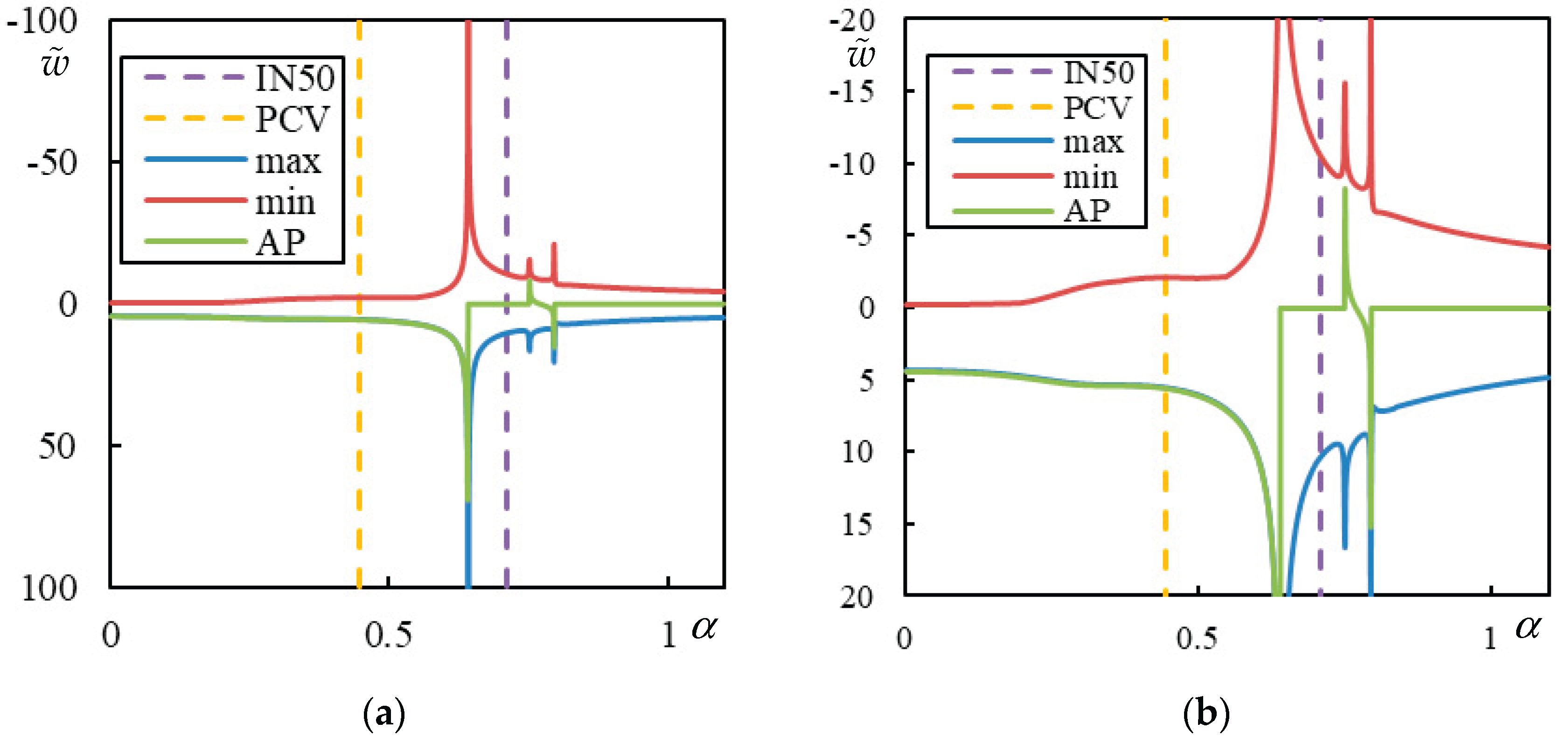
Figure 15.
Probability plot for DOE analysis. As usual, factors are designated A (), B (), C () and D (). Significant effects are indicated in the graph.
Figure 15.
Probability plot for DOE analysis. As usual, factors are designated A (), B (), C () and D (). Significant effects are indicated in the graph.
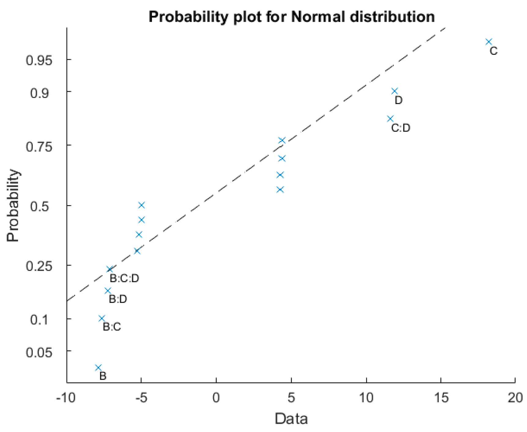
Figure 16.
Analysis related to determination of PI for , , and . In the legend: “peak” (violet) is PCV; “resonance” (red) is ; “asymptote” is at the lowest asymptote to instability lines (orange-1% damping ); “alpha50” is .
Figure 16.
Analysis related to determination of PI for , , and . In the legend: “peak” (violet) is PCV; “resonance” (red) is ; “asymptote” is at the lowest asymptote to instability lines (orange-1% damping ); “alpha50” is .
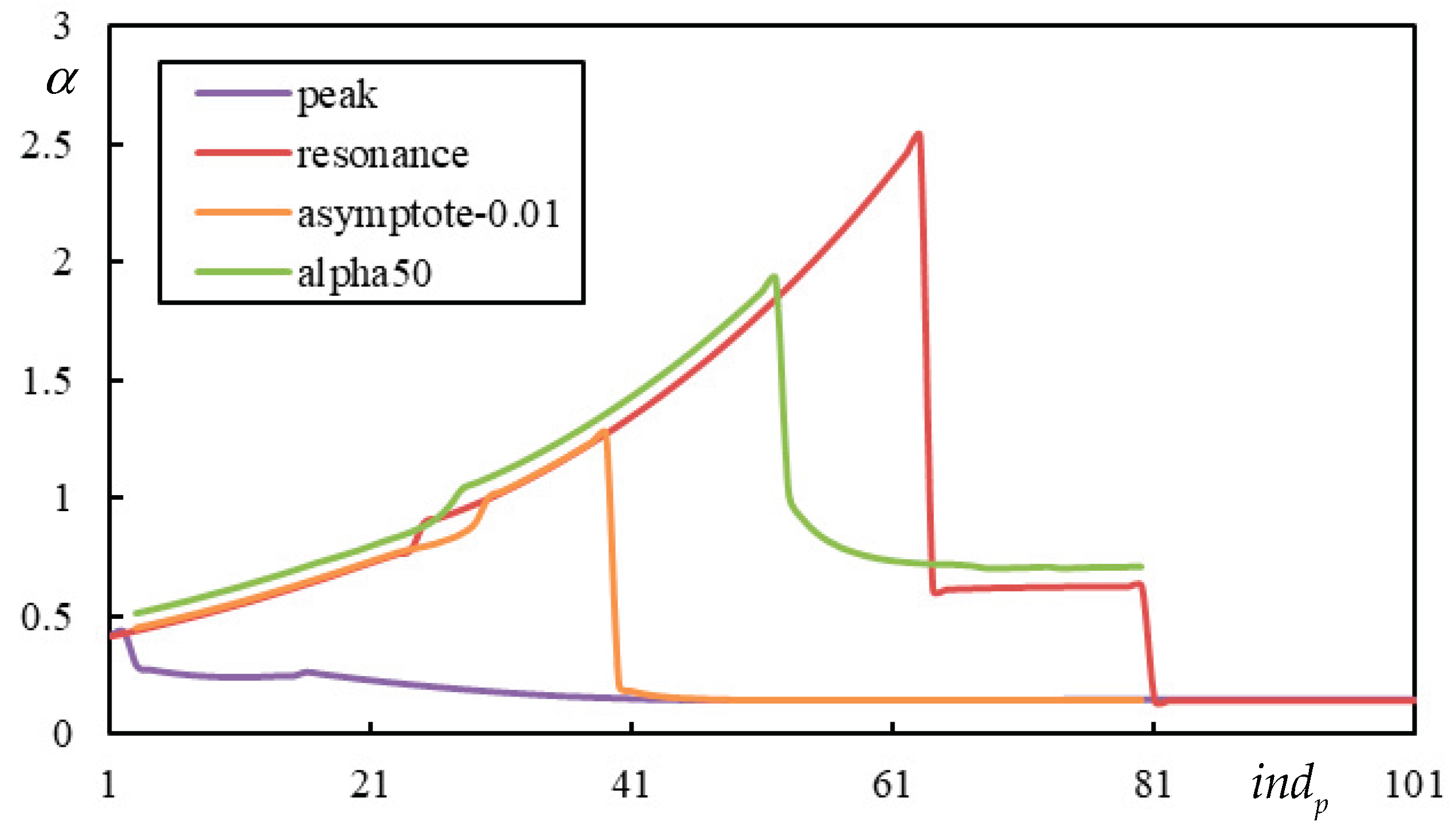
Figure 17.
Final outcome of Monte Carlo analysis and preselection according to (AP – green, Maximum – blue, Minimum – red displacement over the entire beam): , , , and . Parts (a) and (b) refer to different -scale. PCV is marked by an orange dashed line and by a violet dashed line.
Figure 17.
Final outcome of Monte Carlo analysis and preselection according to (AP – green, Maximum – blue, Minimum – red displacement over the entire beam): , , , and . Parts (a) and (b) refer to different -scale. PCV is marked by an orange dashed line and by a violet dashed line.
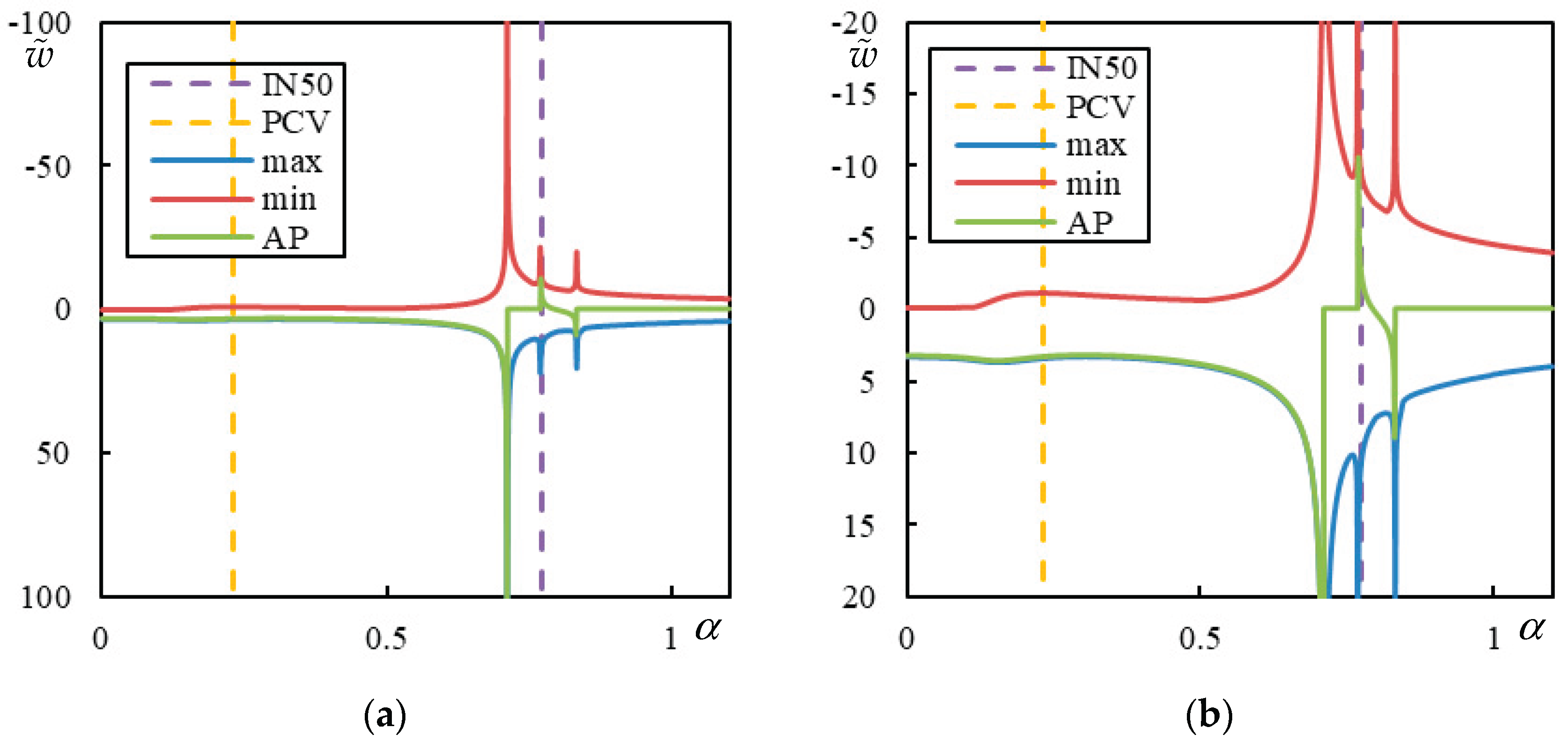
Figure 18.
Parametric search for , , and : (a) preselection according to (b) preselection according to . Different colors correspond to different , with lower values on top.
Figure 18.
Parametric search for , , and : (a) preselection according to (b) preselection according to . Different colors correspond to different , with lower values on top.
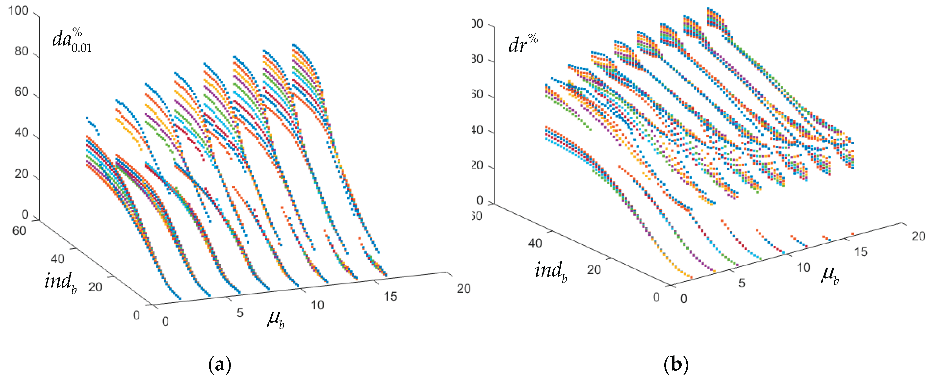
Figure 19.
Parametric search for , , and : (a) preselection according to (b) preselection according to . Different colors correspond to different , with lower values on top.
Figure 19.
Parametric search for , , and : (a) preselection according to (b) preselection according to . Different colors correspond to different , with lower values on top.
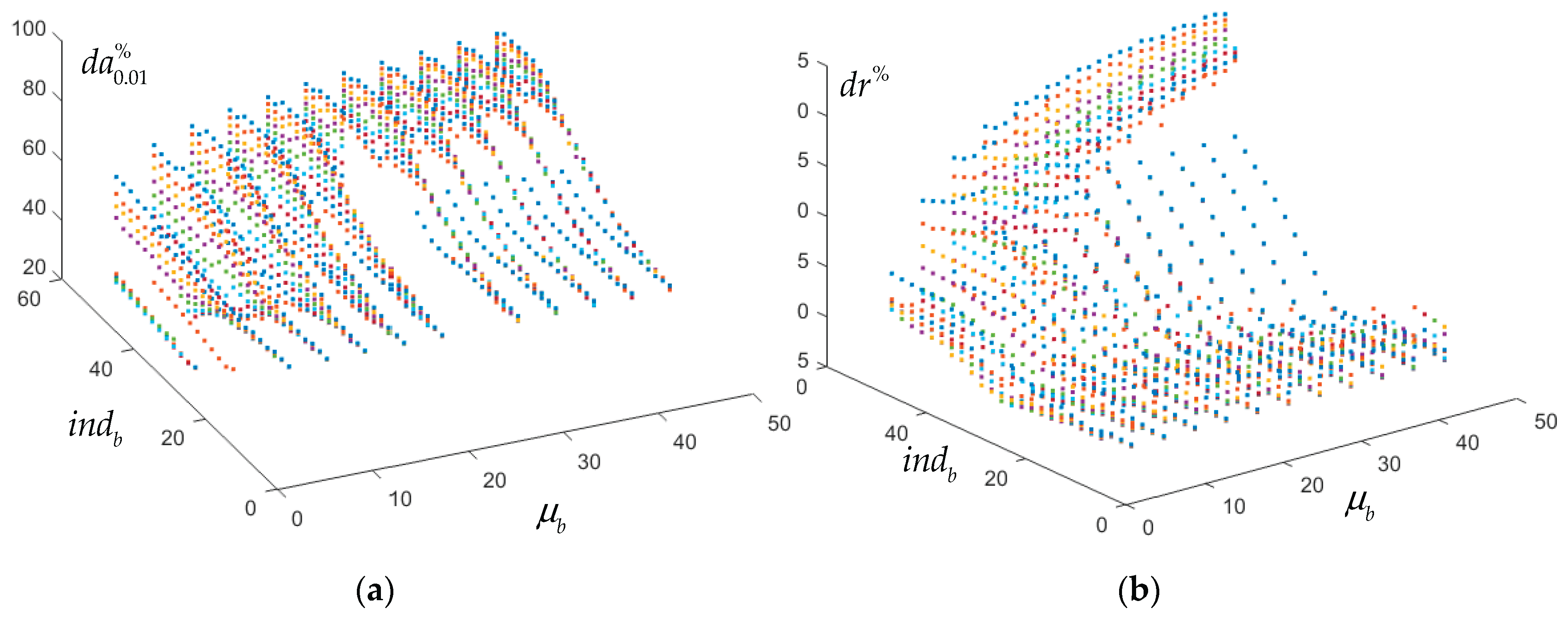
Figure 20.
Final outcome of parametric search for and preselection according to (AP – green, Maximum – blue, Minimum – red displacement over the entire beam):, , and . Parts (a) and (b) refer to different -scale. PCV is marked by an orange dashed line and by a violet dashed line.
Figure 20.
Final outcome of parametric search for and preselection according to (AP – green, Maximum – blue, Minimum – red displacement over the entire beam):, , and . Parts (a) and (b) refer to different -scale. PCV is marked by an orange dashed line and by a violet dashed line.
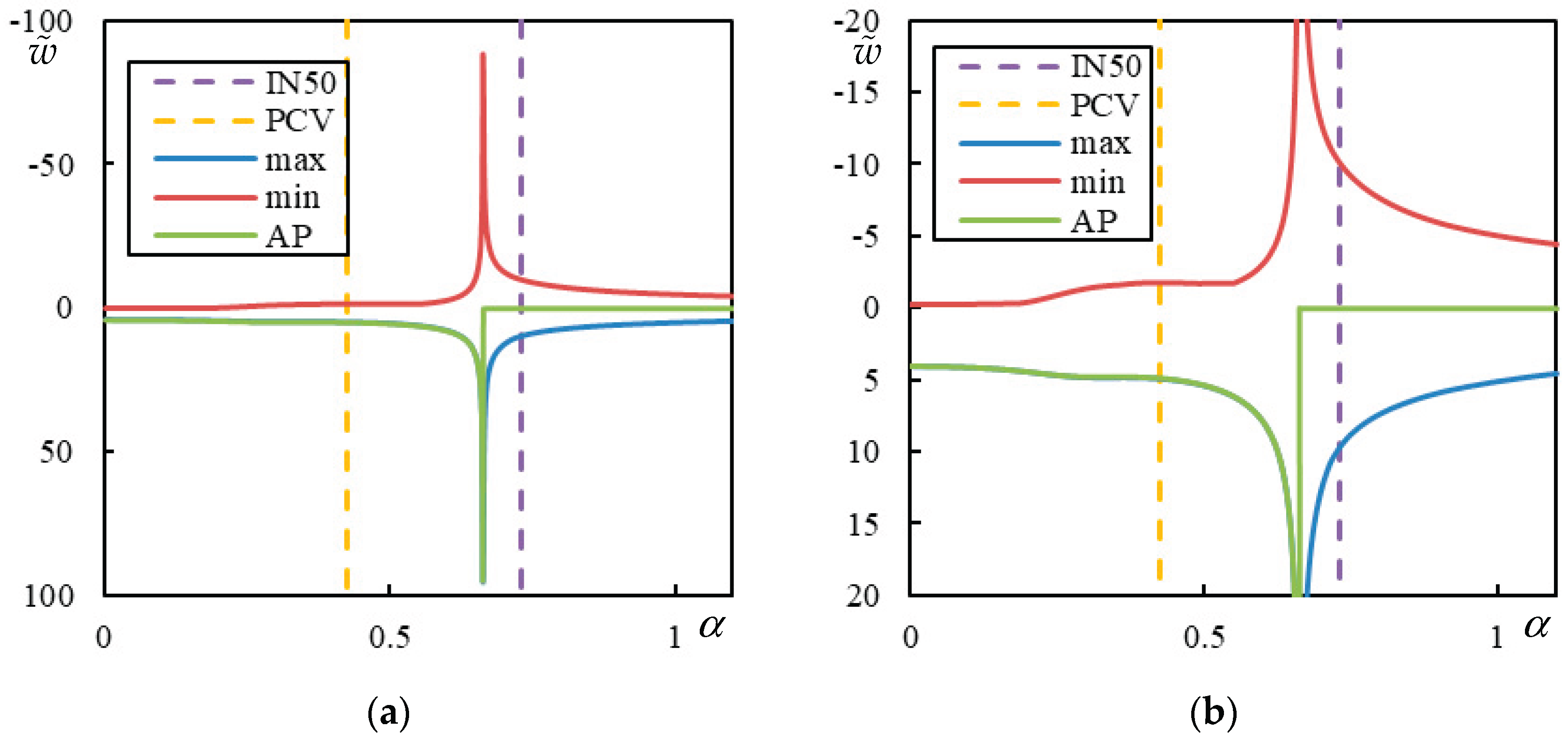
Figure 21.
Final outcome of parametric search for and preselection according to (AP – green, Maximum – blue, Minimum – red displacement over the entire beam): , , and . Parts (a) and (b) refer to different -scale. PCV is marked by an orange dashed line and by a violet dashed line.
Figure 21.
Final outcome of parametric search for and preselection according to (AP – green, Maximum – blue, Minimum – red displacement over the entire beam): , , and . Parts (a) and (b) refer to different -scale. PCV is marked by an orange dashed line and by a violet dashed line.
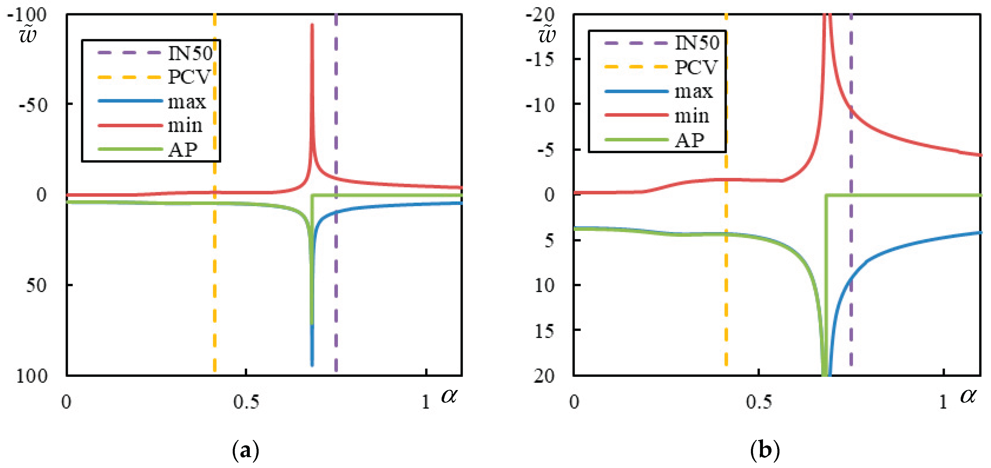
Figure 22.
Final outcome of parametric search for and preselection according to (AP – green, Maximum – blue, Minimum – red displacement over the entire beam): , , and . Parts (a) and (b) refer to different -scale. PCV is marked by an orange dashed line and by a violet dashed line.
Figure 22.
Final outcome of parametric search for and preselection according to (AP – green, Maximum – blue, Minimum – red displacement over the entire beam): , , and . Parts (a) and (b) refer to different -scale. PCV is marked by an orange dashed line and by a violet dashed line.
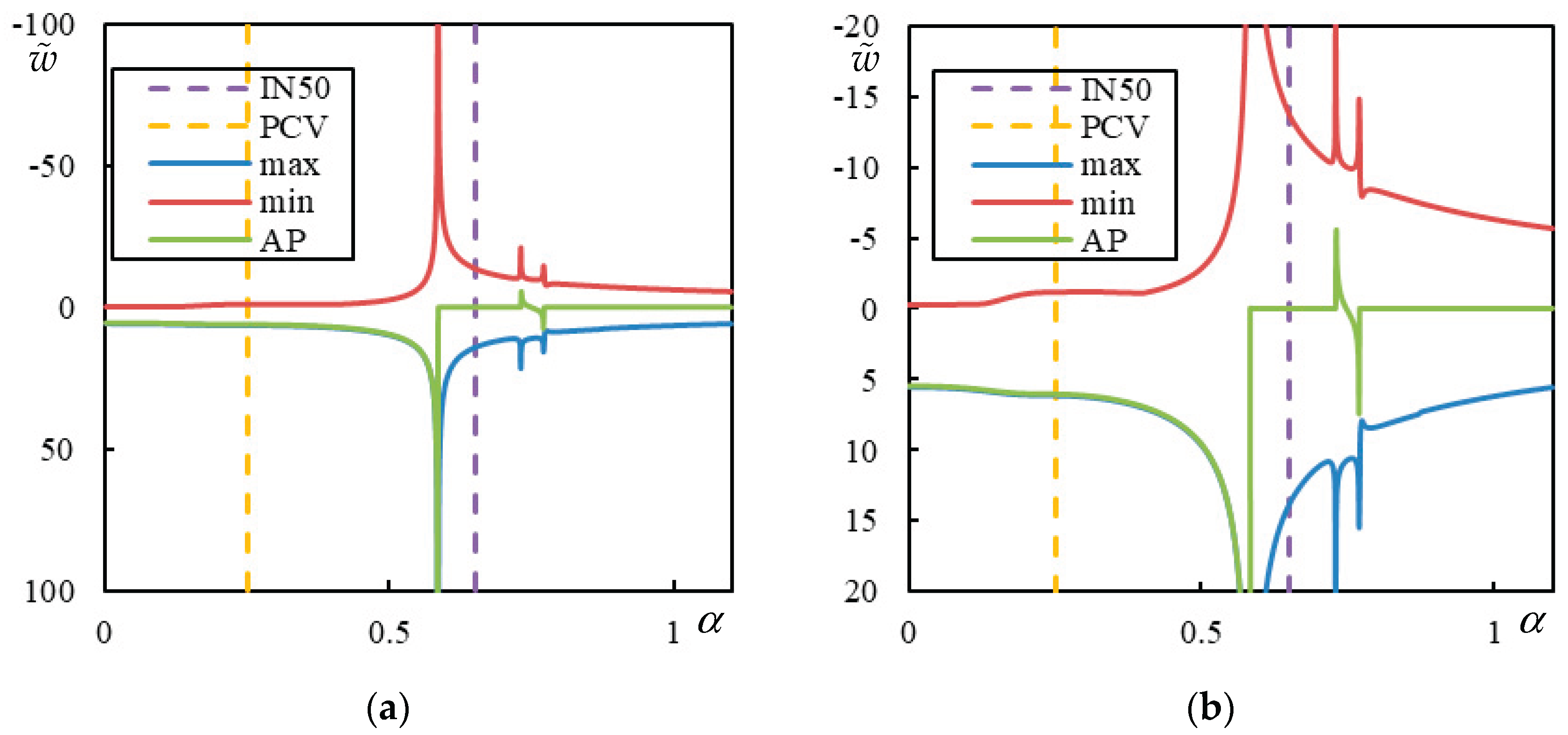
Figure 23.
Final outcome of parametric search for and preselection according to (AP – green, Maximum – blue, Minimum – red displacement over the entire beam): , , and . Parts (a) and (b) refer to different -scale. PCV is marked by an orange dashed line and by a violet dashed line.
Figure 23.
Final outcome of parametric search for and preselection according to (AP – green, Maximum – blue, Minimum – red displacement over the entire beam): , , and . Parts (a) and (b) refer to different -scale. PCV is marked by an orange dashed line and by a violet dashed line.
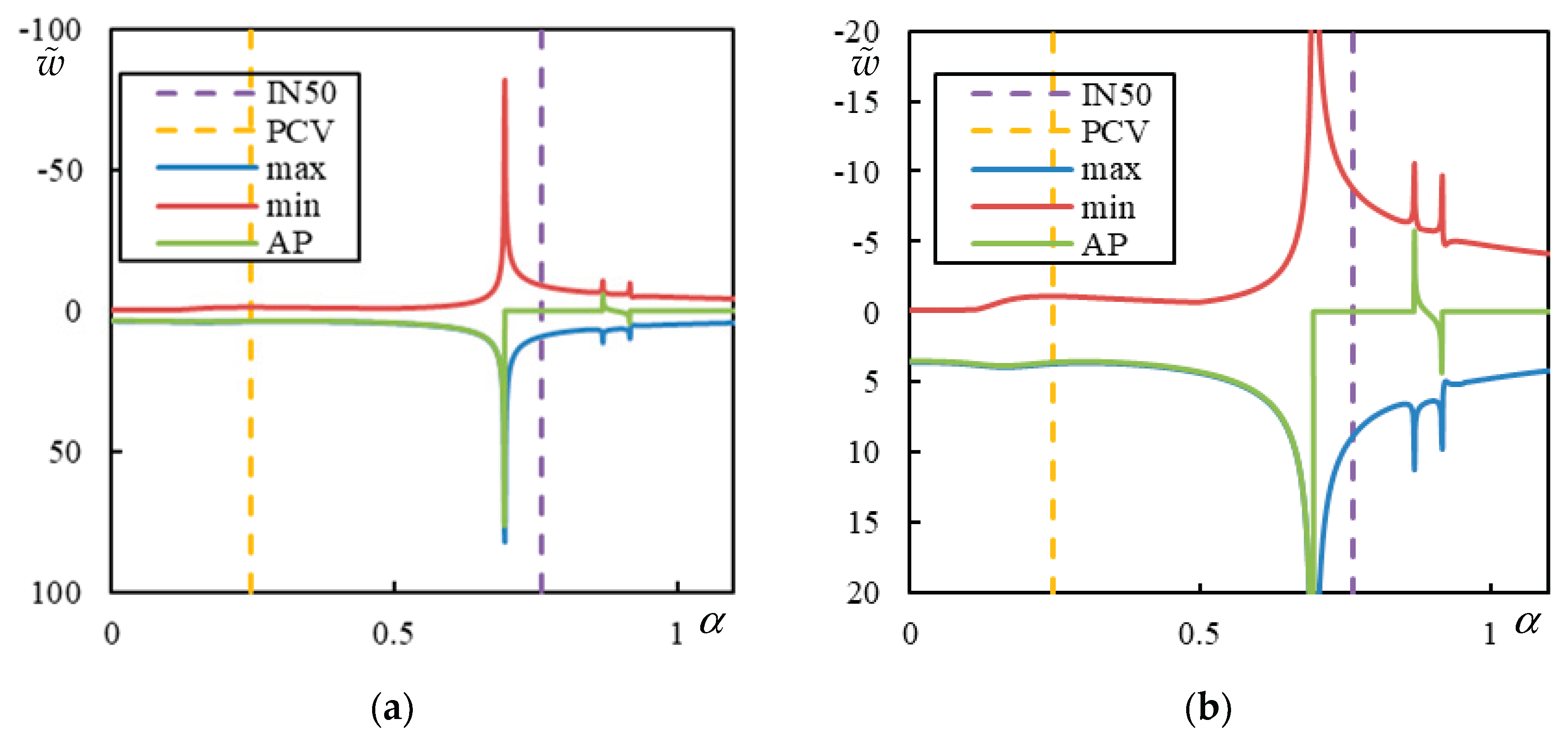
Figure 24.
Summary of different runs of SA: (a) initial set is the best set from MC simulation (5.5244; 44.1292; 44.8870; 0.1111); (b) initial set is the best set from previous simulation; (c) initial set is (4; 15; 30; 0.5).
Figure 24.
Summary of different runs of SA: (a) initial set is the best set from MC simulation (5.5244; 44.1292; 44.8870; 0.1111); (b) initial set is the best set from previous simulation; (c) initial set is (4; 15; 30; 0.5).
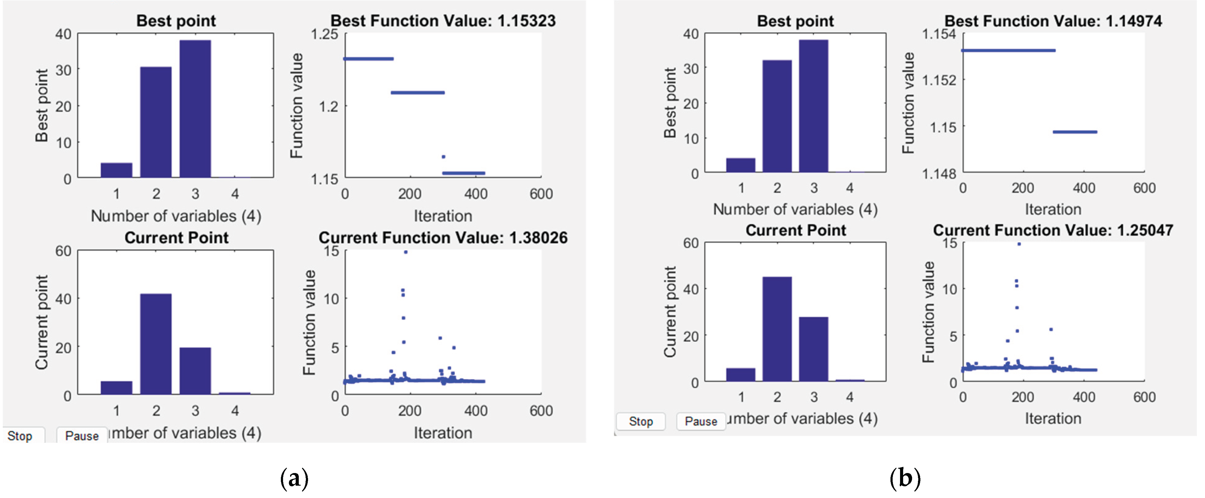
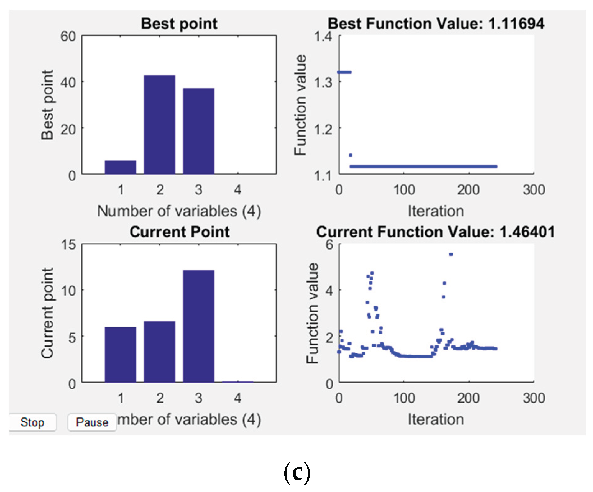
Figure 25.
Analysis related to determination of PI for , , and . In the legend: “peak” (violet) is PCV; “resonance” (red) is ; “asymptote” is at the lowest asymptote to instability lines (orange-1% damping ); “alpha50” is .
Figure 25.
Analysis related to determination of PI for , , and . In the legend: “peak” (violet) is PCV; “resonance” (red) is ; “asymptote” is at the lowest asymptote to instability lines (orange-1% damping ); “alpha50” is .
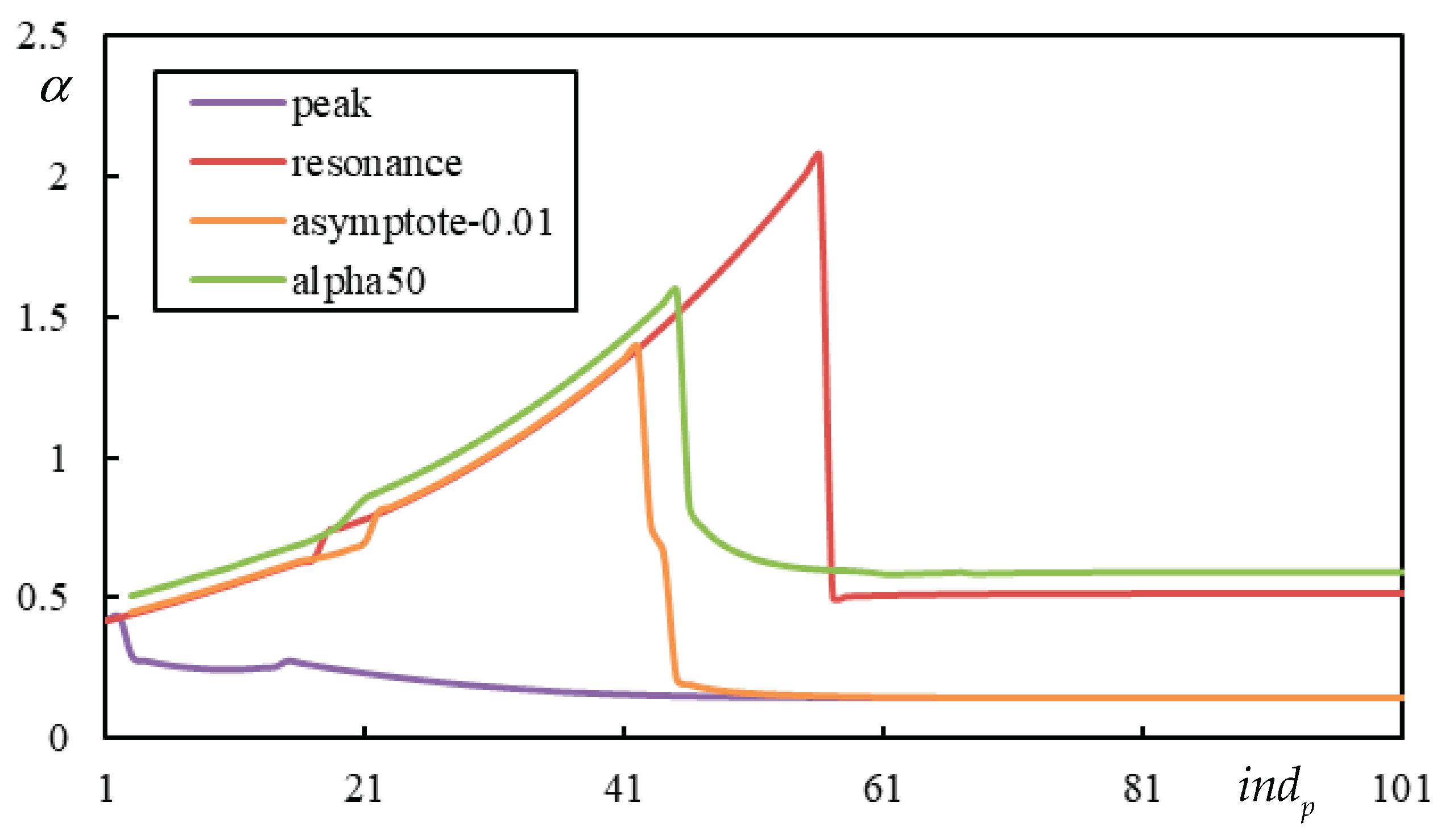
Figure 26.
Final outcome of Simulated Annealing optimization and preselection according to (AP – green, Maximum – blue, Minimum – red displacement over the entire beam): , , ; and . Parts (a) and (b) refer to different -scale. PCV is marked by an orange dashed line and by a violet dashed line.
Figure 26.
Final outcome of Simulated Annealing optimization and preselection according to (AP – green, Maximum – blue, Minimum – red displacement over the entire beam): , , ; and . Parts (a) and (b) refer to different -scale. PCV is marked by an orange dashed line and by a violet dashed line.
Disclaimer/Publisher’s Note: The statements, opinions and data contained in all publications are solely those of the individual author(s) and contributor(s) and not of MDPI and/or the editor(s). MDPI and/or the editor(s) disclaim responsibility for any injury to people or property resulting from any ideas, methods, instructions or products referred to in the content. |
© 2025 by the authors. Licensee MDPI, Basel, Switzerland. This article is an open access article distributed under the terms and conditions of the Creative Commons Attribution (CC BY) license (http://creativecommons.org/licenses/by/4.0/).
Copyright: This open access article is published under a Creative Commons CC BY 4.0 license, which permit the free download, distribution, and reuse, provided that the author and preprint are cited in any reuse.


