
Submitted:
27 September 2025
Posted:
29 September 2025
You are already at the latest version
Abstract
In IEEE 802.11 WLAN networks, the Binary Exponential Backoff (BEB) protocol has been used to avoid collisions due to channel errors, but it is less efficient for dense networks with many transmitting nodes. In this work, we propose a new scheme for adapting the contention window based on the transmission state and random backoff history. We propose four transmission states by aggregating the success or failure status of previous and current transmissions. These states are the conditions for selecting the increasing or decreasing contention window for the subsequent transmission time. The ratio between the random backoff value and the contention window partially determines the amount of change for the new contention window. We use NS-3 simulations to evaluate the performance of our scheme. The results show that the scheme can improve the total throughput and average delay and be more efficient with more nodes.
Keywords:
network technology
; IEEE 802.11
; CSMA/CA protocol
; BEB algorithm
1. Introduction
During the past decade, the tendency for numerous wireless devices to communicate with each other in a specific area has accelerated the development of wireless network technology. IEEE 802.11 wireless technology is widely deployed in WLANs, and its next generations are rapidly developing to support higher data rates, security enhancement, and an increasing number of users. The Distributed Coordination Function (DCF) method of IEEE 802.11 uses the Carrier Sensing Medium Access with Collision Avoidance (CSMA/CA) protocol to control the process of participating stations entering the channel to transmit their packets [1]. The protocol is also called a time-frame control protocol because it uses a Binary Exponential Backoff algorithm (BEB) to generate a deferring time for each station to avoid collisions, and to wait for an opportunity to transmit its packets. The BEB algorithm works efficiently in a low-load or an unsaturated network, where the BEB algorithm guarantees that participating stations send their packets without any collision [2].
However, the BEB implementation causes more collisions when the network becomes dense and hence makes channel access control for stations more challenging [3]. The problem is that after achieving a successful transmission, it resets the contention window (CW) to the minimum backoff interval, which accidentally increases collision probability. In addition, the network delay may be affected by the exponential expansion of the CW size to support packet retransmission after the station suffers a collision [3,4]. Many proposed schemes have focused on adjusting the CW size in the BEB algorithm to improve the CSMA/CA protocol. Even so, finding an optimal CW size for a dynamic wireless network remains an open problem. Typically, some schemes control the CW size to increase or decrease depending on the result of each transmission or the history of transmission times that performed better than the BEB algorithm [5,6,7,8,9,10]. Nevertheless, these schemes mostly expand the CW size after a station which suffered a collision without considering the status of the network load. Therefore, they are ineffective in some cases of rapid change in network loads, and it was difficult for them to reach a theoretical maximum throughput [10]. Besides, some other schemes collect additional information in the network environment to estimate the density of the stations, and then combine them with the result of each transmission to optimize CW size [3,11]. So, they also outperform the BEB algorithm, reduce collisions, obtain high throughput in a saturated network but the obtained CW sizes stayed at high values, which might deteriorate network delay [10]. On the other hand, some research focused on investigating the distribution of random variables in the duration of packet transmission to indicate its influence on network delay [12,13,14].
In this study, we proposed a new scheme to control how to change the size of CW based on the combination of Transmission History and Backoff Probability (named THBP). In our mechanism, the transmission history is expressed by the aggregation of the status (successful or unsuccessful transmission) from two sequent transmissions. In addition, the ratio between the random backoff value (BO) and the CW size defines the backoff probability at the current transmission time. In our scheme, the sizes of CW increase or decrease for subsequent transmissions depends on the transmission history, and the backoff probability.
An internal collision occurs when the BO timers of stations expire simultaneously. The collision is partly due to the CW size, but somehow because of the BO. When a station encounters a collision, the CW size is extended to give the station one more opportunity to retransmit its packet. However, the CW size was at a large value after several times of retransmission, yet the station continues to collide. There are two reasons for this problem: One reason for the CW size was not large enough, and needed to be expanded more, the other reason is that the uniformly random mechanism of BOs leads stations expire simultaneously. In this study, along with using the packet transmission history, we additionally observe the probability of occurrence of the BO in the range of [0, CW - 1] to support the adjustment of CW size more reasonably.
The remaining part of this paper is organized as follows. Section II summarizes the related work. Section III introduces the new scheme. Section IV presents the simulation results are compared to other schemes to evaluate our scheme. Some conclusions are presented in the last section.
2. Related Work
In the CSMA/CA scheme using the BEB algorithm [1], each station generates a uniformly random backoff value (BO) from [0, CW – 1], where the BO is an integer in units of slot time and CW is the size of the contention window. In this algorithm, the CW size is limited in the range of [CWmin, CWmax], and its initial value could be set to CWmin. The values of CWmin, CWmax and slot time are specified in the IEEE 802.11 standard [1]. BO depends on the channel status, and when the BO counts down to zero, the packet is allowed to be sent. The CW size is updated to a new value according to the indication in the acknowledgment and recovery procedures of the CSMA/CA scheme. In the BEB algorithm, the new CW size for the next transmission is obtained in Eq. 1.
where si is defined as a backoff stage at the ith transmission time and , the parameter smax is the maximum times of retransmission. The default value of smax is seven, along with the value of CW corresponding to [16, 32, 64, 128, 256, 512, 1024]. Whenever a station suffers a collision, its CW size is exponentially increased for a retransmission until it catches the value of CWmax or the (2)
In the case of a saturated network, the BEB algorithm performed inefficiently, so Song N.-O et al. proposed a scheme (named exponential increase exponential decrease - EIED) [5], in which the CW size was increased the same as the one in the BEB origin after a collision, and the CW size was divided in half after a successful transmission instead of resetting to CWmin like in the BEB algorithm as in Eq. 1. The new value of CW in this scheme was updated in Eq. 2:
In this scheme, after a station achieved a successful transmission, the size of CW was controlled to gradually decrease to prevent the backoff from falling into a tiny interval. The scheme outperformed the BEB origin. However, in this scheme, CW size was maintained at a high value after a successful transmission, which may be sensitive to throughput and average delay [10]. After that, many other schemes were proposed to improve BEB and surmount the limit of this scheme in the case of dynamic and saturated networks. A proposed scheme named the LILD based on the to adjust the CW size by adding a value of CWmin after a collision of transmission, and by subtracting a value of CWmin after a successful transmission [7]. The speed of changing CW size is slower than that in the EIED scheme because of linear increase or decrease calculations but the LILD scheme is rather effective when the network was dense. However, the scheme caused a network degradation due to the linear decrease of CW size when the network rapidly changed into low loads. Therefore, Ke C. et al. proposed a scheme named SETL to take advantages of the EIED and LILD schemes to improve the BEB algorithm [15]. They used a value of the CW size as a threshold and performed the scheme in a combination of the EIED and LILD schemes. The EIED scheme was performed before the threshold and the LILD was performed after it. The performance of the scheme achieved a low collision rate and a high throughput in comparison to the BEB, EIED and LILD schemes. However, it still failed to reach the maximum throughput due to the setting of CW sizes for networks in saturated condition [10]. Lin C.-H. et al. proposed a scheme named RACB in which the optimal CW sizes were obtained basing on the calculation of collision rate, with the optimal value of collision rate was of 0.1 [10]. The two thresholds of low and high values were pre-defined according to the optimal value in order to combine the performances of the EIED and LILD schemes. The RACB scheme outperformed to the SELT scheme, but many parameters were pre-defined.
Some other proposed schemes presented a new approach to control CW size. Beside using the result of each packet transmission, they extracted more information from the network environment to estimate the network condition. It is valuable when the coming and leaving stations of a network were unknown. Liang H.-M. et al. proposed a PCB (Pause Count Backoff) algorithm used the average number of pauses in the countdown duration to estimate the active stations in the network and then aggregate the estimation result with the result of each transmission to set the appropriate CW size [11]. The scheme’s performance outperformed to the BEB and EIED, especially in fairness. Recently, Ali R. et al. introduced a Channel Observation-based Scaled Backoff scheme (COSB) [3]. In this scheme, they assigned a counter parameter to count the appearance of busy, idle, collision, and success at each slot time in the backoff duration of a station to estimate the channel activities. Then they calculated a collision probability (pcol) as a ratio between the counter parameters and used to control the CW size in combination with the result of each transmission for the subsequent transmission. The CW size was updated in the Eq. 3.
in which ρ was chosen equals to CWmin and pcol is the probability of collision [3].
At first sight, the COSB scheme looked like the EIED scheme when it updated the CW size according to the result of each transmission. However, it became prominent when adding more information about the network environment through the factor pcol. The scheme performed better than the EIED and BEB algorithms, especially when the network became saturated. However, the scheme also created a variety of CW sizes, and the extraction mechanism of pcol was rather complex. In addition, many of the CW sizes were kept at high values to ensure continuously successful transmission, which was a reason for the average delay degradation.
In the past few years, the machine learning algorithms become prior candidates to enhance the CSMA/CA protocol. D. Lee et al. used a method based on a hybrid back-off algorithm that was a combination of the LILD and the EIED schemes with a threshold of CW size to apply the Q-learning algorithm to guarantee the reliability of increasing traffic and to improve the performance in a vehicular network (VANET) [16]. Ali R. et al. had built an iQRA paradigm based on a designed scheme to exploit the optimal actions using Q-learning algorithm, and the CW values were then scaled to those optimal actions for the stations [17]. The performance of the iQRA paradigm was improved in throughput and especially in fairness. However, the trade-off between the exploration and exploitation in Q-learning remains a dilemma [18]. Besides, the Deep Q-learning technique is also approached to optimize the CW size, Wydmanski W. et al. proposed a method called centralized contention window optimization with deep reinforcement learning (CCOD) [19]. The method predicted the CW sizes correctly to maximize the saturation throughput of the system, the inputs of the deep neuron network were the history of collision probabilities, and the output were the optimized rewards which maximized network performance. The obtained results presented an outperformance to the original BEB algorithm in a dense network. Similarly, Zuo Z. et al. employed a Q-learning technique in first phase to obtain the history of collision probabilities, and then a deep neuron network in the second phase to sense the network condition to optimize the CW sizes with a dynamic adjustment in backoff strategy for different access categorie (AC) in an EDCA mechanism [20]. The obtained results presented a better performance than other methods in both normalized throughput and collision rate for differentiating ACs. However, designing a deep neuron network to optimize the parameters in IEEE 802.11 DCF is rather complex and it takes a long time to perform.
In this study, besides using the history of packet transmission, we additionally observe the probability of the BO occurrence during the backoff duration to control the CW size more reasonable for the next transmission. The BO was one of the factors which partly affected the packet transmission result due to its uniform random manner. Our proposal scheme ensures to improve throughput and solve the deterioration of the average delay in case of different network loads. Besides, it is simply in calculation and makes a few alterations to the original BEB algorithm in control the CW size.
3. The Proposal Scheme
In the THBP scheme, we initially estimated the density of a dynamic wireless network based on the results of two consecutive transmission states. We defined Tpc to show ‘previous’ and ‘current’ transmission states, with p and c notated with terms ‘0’ and ‘1’ respectively. The term ‘0’ specified a successful transmission, and ‘1’ indicated that the station had experienced a collision. There are four states (T00, T01, T10, T11), these present the ‘previous’ and ‘current’ transmission states which was successful transmission or collision. Furthermore, we calculate the ratio between the BO value and CW in the current transmission and use it to support the adjustment of CW more reasonable in combination with each transmission state. Mathematically, we defined a backoff probability fi by the ratio
where the BOi was a random backoff value and the CWi size at the ith transmission. We observed the value of fi in combination with four states to define more suitable CW size for the next transmission.
In the case of a saturated network, a small CW size causes more collisions because it increases the probability of the stations falling to the same backoff values. Likewise, if a large CW size was kept in an unsaturated network, the average delay might be deteriorated [10]. Although many schemes were proposed to enhance the BEB algorithm basing on the result of each packet transmission or information from network environment but how the CW size is reasonable to adapt the network condition that is still necessary to investigate and discover. Therefore, we combine the history of two consecutive transmission with the observation of BO through the fi value to adjust the CW size appropriately. In this scheme, we defined si = [0, 1, 2 …, (smax - 1)] as the backoff stages in which smax was the maximum number of retransmitted times as in the BEB algorithm. The increment term of was used to update a new backoff stage after a combination the result of the Tpc and fi observation for stations, and it also specifies the speed change of CW sizes. The backoff stage si was updated to the backoff stage sj as below
Then the new contention window CWj was obtained by:
We observe value of fi to appear in one of three ranges of [0, 0.25), [0.25, 0.5), and [0.5, 1.0]. In the BEB algorithm, the CW is the series of {CWmin, 2 × CWmin, 4 × CWmin, …, CWmax}. At the current CWi, the previous CW are calculated by 0.5 × CWi, 0.25 × CWi, … So, in our scheme, the factors of 1.0, 0.5 and 0.25 were chosen as the upper limit of three ranges above to observe probability fi. It also implies to the BO appearing in any backoff stages of (si - 2), (si - 1) or si. These ranges were normalized in corresponding to BO being small, medium, or large compared to the CW size. Let us discuss the rules for combining Tpc with fi.
In our mechanism, fi is used to partly support the change of CW in each transmission state. When the transmission state presents two sequent collisions (T11). The CW typically needs to expand to avoid collision for the next transmission. However, if fi is small, BO can be larger in the next round with the current CW size. It means that the collision can be solved without changing the backoff stage, and the CW remains unchanged. If fi is medium, the current CW size is necessary to extend a reasonable amount to support the average delay of the network. If fi is large, it implies that the BO is proportional to the CW size, and we should increase a large amount of the CW size to avoid collision in the subsequent transmission. In the case of the transmission state changes from success to collision (T01), the BEB algorithm increases the CW size by twice to increase the BO value to avoid collision in the next round. However, in our mechanism, if the fi is small, BO can be larger in the next round with the current CW size, thus its size remains at this backoff stage. If the fi is medium or large, the CW is doubled, similar to the BEB algorithm, to support a suitable BO value for the next transmission. Likewise, when the transmission state presents two sequent successes (T00). If fi is large, the CW size is reasonable at this backoff stage and is unchanged. If the fi is small and medium, the CW size decreases a small amount to avoid an unnecessary delay for the backoff duration. In the case of transmission state changes from collision to success (T10), instead of decreasing to the previous backoff stage, CW size still remains at this backoff stage with any values of fi to avoid more collisions in the next round.
The factor Δpc in equation (5) was described by
where (s), (m), (l) correspond to small, medium, and large, respectively. The value of factor Δpc is used to define the next backoff stage. We present the predicted values of Δpc in Table 1.
Table 1 shows that the state T00 specifies the transmission state to be successful twice, and the value of fi < 0.5 refers to a small BO value. Therefore, CW should be smaller, and the backoff stage si reduces to si -1 by the setting . If fi > 0.5, it implies that the current CW size was large enough and should remain unchanged, as .
In the state T10, which means that the transmission state changes from collision to a success, then the backoff stage si is good enough. So, CW size is kept unchanged with any values of fi and , and are set to zero. Then, the backoff stage si can be changed in the next round.
In the state T01, it refers to a success accompanied by a collision. If fi < 0.25, it implies that the collision of the current transmission time was not due to the size of CW, and the backoff stage si should remain unchanged, and was set to zero. Only if fi > 0.25, the CW size needed to be increased to the CW size at the backoff stage si + 1, so we set both and to equal +1.
In the state of T11, which indicates two consecutive collisions. If fi > 0.5, this means that the CW size and the BO value were rather high, but the station has continuously suffered a collision. Therefore, the CW size needed to be expanded a lot, and here the appropriate factor should be +2, which referred to the CW size at the backoff stage jumped to the backoff stage si + 2. If 0.25 ≤ fi < 0.5, the CW size needed to expand a few, we thus predicted to increase the CW size in the backoff stage si to the backoff stage si + 1 and set the factor to be +1. For the case fi < 0.25, we kept the CW size unchanged and set the factor to be zero.
Likewise, we describe the transition of the CW among backoff stages according to the factor Δpc in the diagram in Figure 1 with the pseudo-codes in the Algorithm 1.
In Figure 1, the CW size is at each retransmission time of the BEB algorithm, which was described in Section 2. The CW size is updated in this scheme presented in Equation 8.
| Algorithm 1. The pseudo-codes of THBP scheme. | |
| 1: | Procedure update_contention_window |
| 2: | fi = BOi/(CWi + 1) // using Eq. (4) |
| 3: | If (previous_transư is successful AND current_trans is successful) then |
| 4: | If (fi < 0.25) then |
| 5: | Deltapc = − 1 |
| 6: | Elseif (fi ≥ 0.25 AND fi < 0.5) then |
| 7: | Deltapc = -1 |
| 8: | Elseif (fi ≥ 0.5) then |
| 9: | Deltapc = 0 |
| 10: | ElseIf (previous_trans is successful AND current_trans is failed) then |
| 11: | If (fi < 0.25) then |
| 12: | Deltapc = 0 |
| 13: | Elseif (fi ≥ 0.25 AND fi < 0.5) then |
| 14: | Deltapc = 0 |
| 15: | Elseif (fi ≥ 0.5) then |
| 16: | Deltapc = 0 |
| 17: | ElseIf (previous_trans is failed AND current_trans is successful) then |
| 18: | If (fi < 0.25) then |
| 19: | Deltapc = 0 |
| 20: | Elseif (fi ≥ 0.25 AND fi < 0.5) then |
| 21: | Deltapc = 1 |
| 22: | Elseif (fi ≥ 0.5) then |
| 23: | Deltapc = 1 |
| 24: | ElseIf (previous_trans is failed AND current_trans is failed) then |
| 25: | If (fi < 0.25) then |
| 26: | Deltapc = 0 |
| 27: | Elseif (fi ≥ 0.25 AND fi < 0.5) then |
| 28: | Deltapc = 1 |
| 29: | Elseif (fi ≥ 0.5) then |
| 30: | Deltapc = 2 |
| 31: | Update sj ← si // using Eq. (5) |
| 32: | Update CWj = CWmin × 2^sj // using Eq. (6) |
| 33: | Update previous_trans ← current_trans |
| 34: | END procedure |
The proposed THBP scheme guarantees to obtain high throughput, low delay, good fairness, and address the sensitive delay that the EIED and COSB schemes encountered. The scheme contributed to minimizing collisions and improving the network performance for different network loads. Moreover, our scheme requests a little computational resource by adding a few conditional statements (see in the pseudo-codes). In comparison to the BEB algorithm, our scheme only uses two new integer variables that are updated after each transmission, the first one is the previous state of transmission which is either 0 or 1, the second one is the transmission stage si ∈ [0, smax - 1] with smax is a tiny integer number. Hence, no overhead traffic is added.
4. Experiment
In this section, we evaluated the efficiency of the THBP scheme through simulations using the NS3 tool, version 3.36.1 [21]. In addition, the simulation results of the THBP scheme were compared to those of the BEB algorithm and the EIED, COSB schemes by measuring aggregated throughput, average delay, fairness index and packet loss rate in a network with varying load conditions.
In this simulation, we set up topologies of an ad-hoc grid and a mobile ad-hoc network (MANET) to investigate the efficiency of controlling CW at the MAC layer of IEEE 802.11. Ad-hoc grid and MANET networks, which are wireless networks without infrastructure, are typically designed to accomplish a specific task such as disaster management, military, rescue operations, etc. An ad-hoc grid topology is stable in sharing the resources among nodes, although its nodes are coming and leaving constantly. The nodes in these topologies can be mobile devices, software, and support devices with wireless connectivity. Moreover, the MANET networks with their flexibility and adaptability are applied in environmental monitoring, healthcare, home automation, sensor and vehicular networks, etc.
4.1. Simulation Results on an Ad-Hoc Grid Topology
In this ad-hoc grid topology, we set the five base stations at the center in fixed positions. Then, five to fifty source stations were put in the grid in random positions, with five stations gradually added by each step. The distance between the two stations was about 25 meters in an area of m. We assumed that the competing stations (STAs) always had packets to transmit to express saturation conditions. We ran 20 simulation trials with 5 to 50 competing stations and averaged the results. The simulation parameters are shown in Table 2.
Initially, we use the simulation parameters in Table 2 to simulate the BEB, the EIED, the COSB, and the THBP schemes on this topology to evaluate our scheme. The simulation results are presented in Figure 2(a), (b), (c). Figure 2(a) showed that when the competing stations were less than 15, the THBP performed as well as the BEB algorithm, and their throughput results are nearly the same. However, there is a contrast between them when the competing stations are more than 15. The throughput of the BEB algorithm decreases rapidly, while the throughput of the THBP scheme continues to increase until the number of stations reaches 20. When the number of stations is more than twenty, the THBP’s throughput reduces due to more collisions occurring. The BEB algorithm expressed a rapid decrease in throughput from nearly 22 Mbit/s to 18 Mbit/s, which refers to the BEB algorithm facing a rapid increase in collision rate. Besides, Figure 2(a) also describes the stable implementation of the THBP scheme along with the BEB, where the throughput of the THBP scheme was about 5 Mbit/s better than that of the BEB at each step of increasing the number of transmitting stations. It should be noted that the enhanced schemes typically increased the CW size after a station suffered a collision and decreased the CW size after a station achieved a successful transmission. However, if a station has just achieved a successful transmission at the backoff stage and still has more packets to send but the CW size is controlled in decrease. The decrease may push the station in a collision because the CW size is not large enough for the next transmission. Therefore, the reasonable change of CW size in the THBP scheme is crucial to specify the enough time for stations achieving more times of successful packet transmission instead of experiencing more retransmission. Figure 2(a) showed that the EIED, COSB perform more effectively than the BEB algorithm in throughput, but the THBP model achieves the highest throughput of all. The throughput of the THBP scheme was approximately 2 Mbit/s better than that of the EIED scheme and more than 1 Mbit/s better than that of the COSB scheme for 20 or more competing stations.
Furthermore, Figure 2(b) presents the average delay results of the compared schemes. The THBP scheme outperformed the BEB algorithm in the average delay of the network. Consequently, the THBP scheme has effectively dealt with the increasing collision rate, which the BEB algorithm suffered. Although the throughput of the COSB scheme was superior to that of the EIED and BEB, it experienced a deterioration in the average delay because it mostly kept the sizes of CW at large values due to multiplication during the process of updating the CW size. The average delay result of the THBP scheme was dominant over the results of the EIED and COSB schemes. The appropriate adjustment of the CW size, supported by the fi values, was a key component in reducing the average delay of the network in this scheme. The THBP scheme expresses a prominent performance in both throughput and average delay, especially in the case of a saturated network. In addition, we investigate the fairness index of each scheme by calculating the fairness index following Jain’s fairness [22]. It is an important measure in a wireless network to specify a fair resource allocation for each station, and is an essential element contributing to the efficiency of network performance. Figure 2(c) shows that the fairness indexes in the compared schemes are approximately the same. Finally, the packet loss rate is also taken into account and the results are presented in the Figure 2(d), the THBP scheme presents the best result in comparison to those of other schemes. In general, the simulated results showed that the reasonable adaptation of the CW size brings the best throughput, average delay, packet loss rate while maintaining a good fairness index to the THBP scheme.
4.2. Simulation Results on a MANET Topology
In this MANET topology, we use a random waypoint mobility model for station mobility at a speed of 2m/s without pause time, and the other parameters are in Table 2. The transmitting stations (from 5 to 40 stations) are randomly distributed in an area with a constant density based on the total number of stations, and the five sink stations are in fixed positions. The simulated results are presented in Figure 3.
The simulated results in this topology are nearly similar to the results in the ad hoc grid topology. Figure 3(a) shows that the throughput obtained from the THBP scheme is the best result compared to the BEB, EIED, COSB schemes. Figure 3(b) presents the average delay of the THBP scheme which is superior to the compared schemes. In addition, the fairness indices of the compared schemes, which are shown in Figure 3(c), are approximate to each other in a good performance for the network. Figure 3(d) presents that the packet loss rates of the THBP and EIED and COSB schemes are nearly approximate to each other and better than the one of the BEB algorithm. However, the THBP scheme still presents as the best scheme in the result of packet loss rate. Therefore, the THBP scheme performs efficiently on both topologies and indicates a better enhancement to the BEB, EIED, and COSB schemes.
5. Conclusions
In this paper, we have proposed a new THBP scheme that adjusts the CW size based on the information available from the consecutive transmission, the BO, and the CW history. The THBP scheme only makes a minor change to the active mechanism of the CSMA/CA protocol. The simulated results in both topologies showed that the THBP scheme specifies a better performance compared to the BEB, EIED, and COSB schemes, and surpasses them in both throughput and average delay, packet loss rate, and along with its approximate fairness. Moreover, the average delay of the THBP scheme also specifies that the scheme partially solves the issue of delay deterioration that many schemes experienced in the case of different network loads.
In conclusion, the efficiency of a dynamic wireless network in IEEE 802.11 DCF depended on the design of the BEB algorithm. However, the methods from the traditional approaches were applied to control the CW sizes is gradually obsolete, and the enhancement of the protocol has been applied by new techniques in recent years [23]. Therefore, we would continue to focus on improving our scheme by applying new techniques and pay attention on the IEEE 802.11e with different kinds of the packet in our future work.\
Declaration of competing interest
The authors declare that they have no known competing financial interests or personal relationships that could have appeared to influence the work reported in this paper.
Acknowledgements
The research funding from Vietnam Academy of Science and Technology (VAST) under grant number NVCC02.05/25-25 was acknowledged.
References
- The 802.11 Working Group, “Chapter 10 - Part 11: Wireless LAN MAC and PHY Specifications,” in IEEE Std 802.11TM-2016, New York, 2016, pp. 1296–1574.
- Vijay K. Garg, “Chapter 21 – Wireless Communications and Networking,” in Wireless Communications and Networking, Elsevier Inc., San Francisco: Morgan Kaufmann Publishers, 2007, pp. 713–775.
- R. Ali, N. Shahin, Y. -T. Kim, B. -S. Kim, and S. W. Kim, “Channel observation-based scaled backoff mechanism for high-efficiency WLANs,” Electron Lett, vol. 54, no. 10, pp. 663–665, May 2018. [CrossRef]
- L. Dai and X. Sun, “A Unified Analysis of IEEE 802.11 DCF Networks: Stability, Throughput, and Delay,” IEEE Trans Mob Comput, vol. 12, no. 8, pp. 1558–1572, Aug. 2013. [CrossRef]
- Nab-Oak Song, Byung-Jae Kwak, Jabin Song, and L. E. Miller, “Enhancement of IEEE 802.11 distributed coordination function with exponential increase exponential decrease backoff algorithm,” in The 57th IEEE Semiannual Vehicular Technology Conference, 2003. VTC 2003-Spring., IEEE, pp. 2775–2778. [CrossRef]
- Nafaa, A. Ksentini, and A. Mehaoua, “SCW: sliding contention window for efficient service differentiation in IEEE 802.11 networks,” in IEEE Wireless Communications and Networking Conference, 2005, IEEE, 2005, pp. 1626-1631 Vol. 3. [CrossRef]
- M. Bharatiya and S. Prasad, “MILD based sliding contention window mechanism for QoS in Wireless LANs,” in 2008 Fourth International Conference on Wireless Communication and Sensor Networks, IEEE, Dec. 2008, pp. 105–110. [CrossRef]
- Q. Nasir and M. Albalt, “History Based Adaptive Backoff (HBAB) IEEE 802.11 MAC Protocol,” in 6th Annual Communication Networks and Services Research Conference (cnsr 2008), IEEE, May 2008, pp. 533–538. [CrossRef]
- S. Manaseer and F. Badwan, “History-Based Backoff Algorithms for Mobile Ad Hoc Networks,” Journal of Computer and Communications, vol. 04, no. 11, pp. 37–46, 2016. [CrossRef]
- C.-H. Lin, M.-H. Cheng, W.-S. Hwang, C.-K. Shieh, and Y.-H. Wei, “A Rapidly Adaptive Collision Backoff Algorithm for Improving the Throughput in WLANs,” Electronics (Basel), vol. 12, no. 15, p. 3324, Aug. 2023. [CrossRef]
- H.-M. Liang, S. Zeadally, N. K. Chilamkurti, and C.-K. Shieh, “A Novel Pause Count Backoff Algorithm for Channel Access in IEEE 802.11 Based Wireless LANs,” in International Symposium on Computer Science and its Applications, IEEE, Oct. 2008, pp. 163–168. [CrossRef]
- Zanella and F. De Pellegrini, “Statistical characterization of the service time in saturated IEEE 802.11 networks,” IEEE Communications Letters, vol. 9, no. 3, pp. 225–227, Mar. 2005. [CrossRef]
- Banchs, P. Serrano, and A. Azcorra, “End-to-end delay analysis and admission control in 802.11 DCF WLANs,” Comput Commun, vol. 29, no. 7, pp. 842–854, Apr. 2006. [CrossRef]
- M. E. Rivero-Angeles, D. Lara-Rodriguez, and F. A. Cruz-Perez, “Gaussian approximations for the probability mass function of the access delay for different backoff policies in S-ALOHA,” IEEE Communications Letters, vol. 10, no. 10, pp. 731–733, Oct. 2006. [CrossRef]
- Ke, C. Wei, K. W. Lin, and J. Ding, “A smart exponential-threshold-linear backoff mechanism for IEEE 802.11 WLANs,” International Journal of Communication Systems, vol. 24, no. 8, pp. 1033–1048, Aug. 2011. [CrossRef]
- Lee, Y. Deng, and Y.-J. Choi, “Back-off Improvement By Using Q-learning in IEEE 802.11p Vehicular Network,” in 2020 International Conference on Information and Communication Technology Convergence (ICTC), IEEE, Oct. 2020, pp. 1819–1821. [CrossRef]
- R. Ali, N. Shahin, Y. Bin Zikria, B.-S. Kim, and S. W. Kim, “Deep Reinforcement Learning Paradigm for Performance Optimization of Channel Observation–Based MAC Protocols in Dense WLANs,” IEEE Access, vol. 7, pp. 3500–3511, 2019. [CrossRef]
- Richard, S. Sutton and Andrew G. Barto, Reinforcement Learning: An Introduction. The MIT Press, 2014.
- W. Wydmanski and S. Szott, “Contention Window Optimization in IEEE 802.11ax Networks with Deep Reinforcement Learning,” in 2021 IEEE Wireless Communications and Networking Conference (WCNC), IEEE, Mar. 2021, pp. 1–6. [CrossRef]
- Z. Zuo, D. Wang, X. Nie, X. Pan, M. Deng, and M. Ma, “PDCF-DRL: a contention window backoff scheme based on deep reinforcement learning for differentiating access categories,” J Supercomput, vol. 81, no. 1, p. 213, Jan. 2025. [CrossRef]
- ns-3 simulator, “https://www.nsnam.org/.”.
- M. C. and W. H. R. Jain, “A quantitative measure of fairness and discrimination for resource allocation in shared computer system,” Maynard, MA, USA, Sep. 1984.
- S. Szott et al., “Wi-Fi Meets ML: A Survey on Improving IEEE 802.11 Performance With Machine Learning,” IEEE Communications Surveys & Tutorials, vol. 24, no. 3, pp. 1843–1893, 2022. [CrossRef]
Figure 1.
The diagram of the CW size transition following the factor Δpc among the backoff stages.
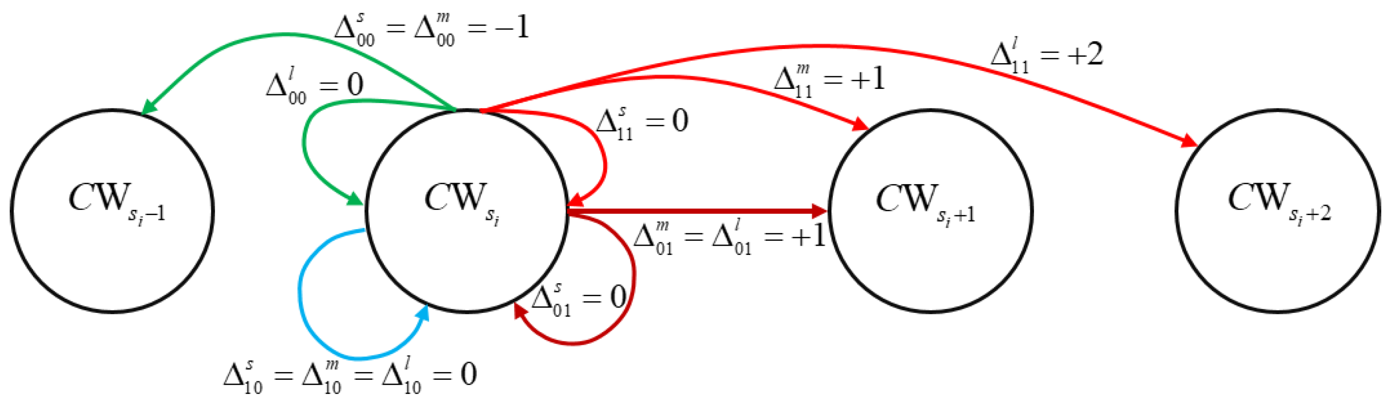
Figure 2.
The simulated results of the compared scheme on an ad hoc grid topology.
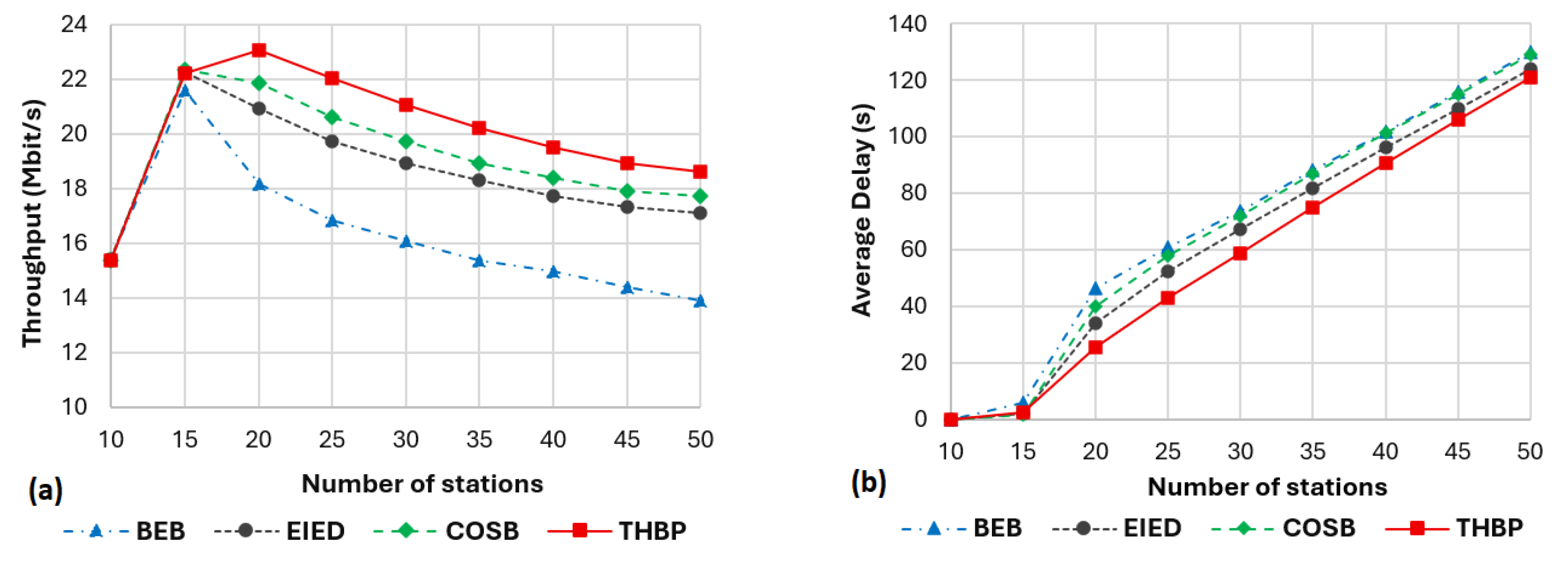
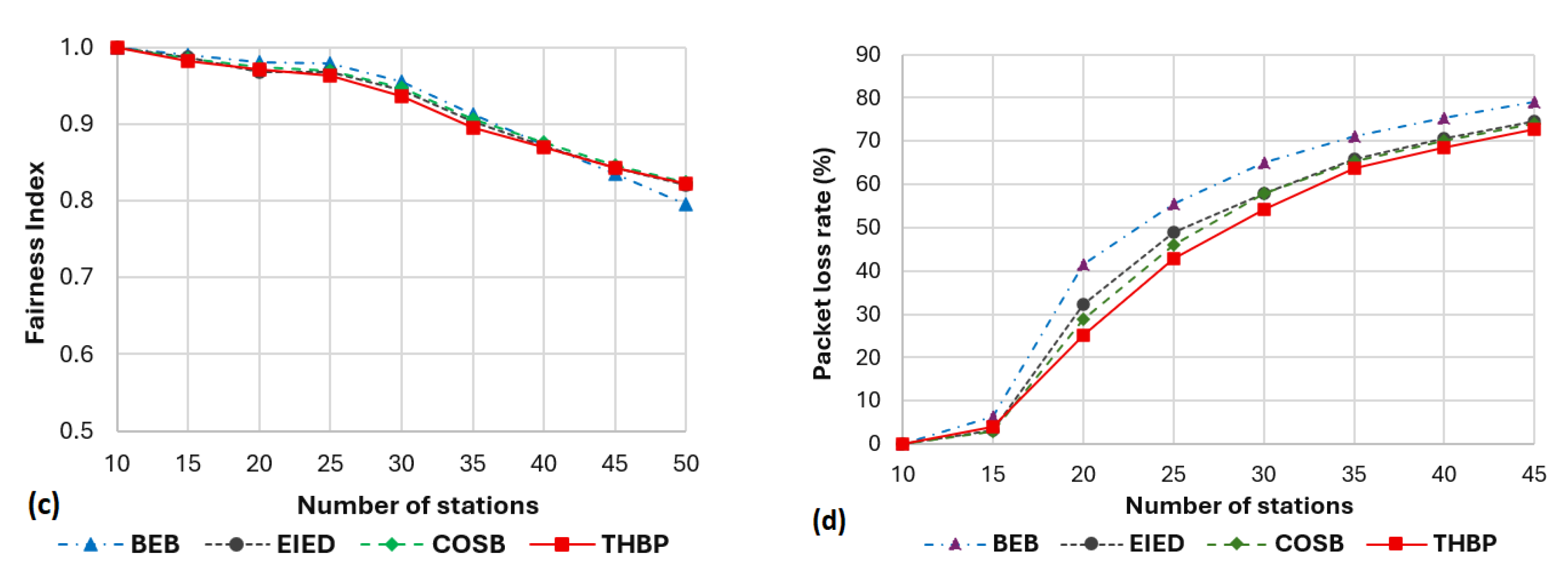
Figure 3.
The simulated results of the compared schemes on a MANET topology.
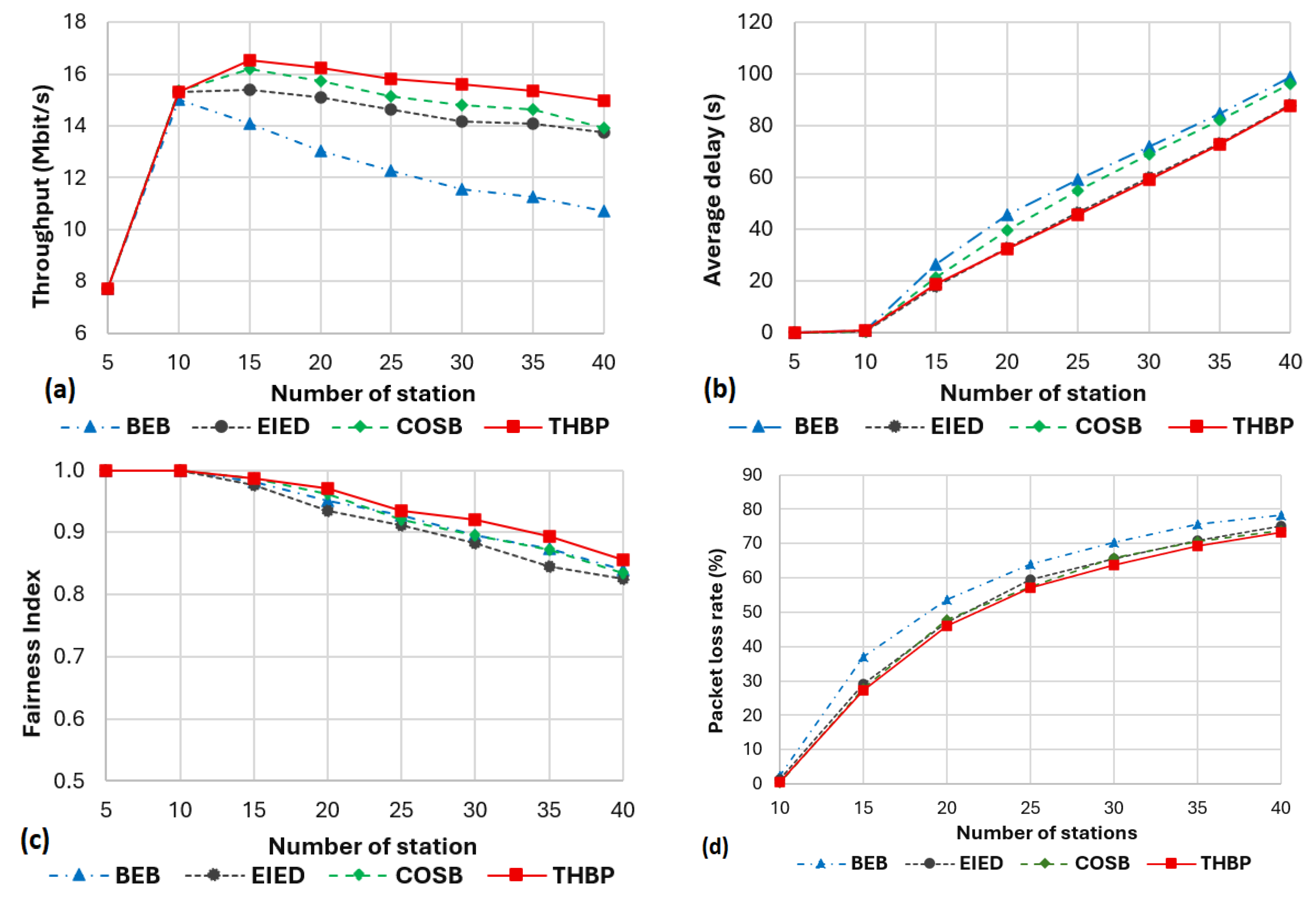

Table 1.
The predicted values of the factor Δpc corresponded to each state.
| States | fi | ||
| Small | Medium | Large | |
| T00 | |||
| T10 | |||
| T01 | |||
| T11 | |||
Table 2.
The simulation parameters.
| Parameters | Values | Parameters | Values |
| Operating Frequency | 5 GHz | CWmin | 31 |
| Bandwidth | 20 MHz | CWmax | 1023 |
| Packet size | 1024 bytes | Stations | From 5 to 50 |
| aSlottime | 9 μs | PropagationLossModel | LogDistance |
| Datarate | 54Mbps | Distance between stations | From 20 to 25 m |
| Packet rate | 300 kbps | Routing Protocol | Optimized Link State Routing |
Disclaimer/Publisher’s Note: The statements, opinions and data contained in all publications are solely those of the individual author(s) and contributor(s) and not of MDPI and/or the editor(s). MDPI and/or the editor(s) disclaim responsibility for any injury to people or property resulting from any ideas, methods, instructions or products referred to in the content. |
© 2025 by the authors. Licensee MDPI, Basel, Switzerland. This article is an open access article distributed under the terms and conditions of the Creative Commons Attribution (CC BY) license (http://creativecommons.org/licenses/by/4.0/).
Copyright: This open access article is published under a Creative Commons CC BY 4.0 license, which permit the free download, distribution, and reuse, provided that the author and preprint are cited in any reuse.


