
Submitted:
30 June 2025
Posted:
30 June 2025
You are already at the latest version
Abstract
Displacement measurement is a critical issue in mechanical engineering. The moiré effect increases the accuracy of contactless measurements. We theoretically estimated the sensitivity threshold of moiré measurements using a digital camera on various objects. The estimated sensitivity threshold can be as low as a sub-pixel. We confirmed this experimentally in laboratory tests with a static image on a screen and simulated movement with non-integer and fractional amplitudes. We also provide practical examples of displacement measurement in the laboratory and outdoors (bridges and cars). Simultaneous measurements were made in two directions. The results can be used in public safety, in particular for monitoring the condition of engineering structures.
Keywords:
moiré effect
; moiré measurements
; moiré sensitivity
; public safety
; moiré sensor
1. Introduction
The moiré effect is an optical interaction between superimposed layers with periodically modulated transmittance [1]. The moiré effect has been extensively investigated in optics [2,3,4,5,6].
The moiré patterns in superimposed (overlapped) regular or nearly regular structures (arrays) appear as light and dark interference fringes, which look like repeated lines, circles, or dots, depending on the geometry of the layers. The moiré effect occurs when “repetitive structures (such as screens, grids or gratings) are superposed or viewed against each other” [1]. Important is “a new pattern of alternating dark and bright areas which is clearly observed at the superposition, although it does not appear in any of the original” [1]. Also, it was noted [7] that “the moiré effect denotes a fringe pattern formed by the superposition of two grid structures of similar period.” When black (opaque) lines of one array are superimposed on white (transparent) spaces between the lines of another array, dark (on average) areas of moiré patterns are formed, and when the black lines of both objects coincide, light moiré areas are formed. The moiré effect is the formation of patterns with longer periods by interference between similar periodic structures with shorter periods, followed by averaging [8]. The studies [1,9,10,11] provide a solid theoretical basis.
The period of the moiré patterns is longer than that of overlapping structures [1]. The moiré is a formation of large-scale patterns (bands or fringes) owing to the interference between similar periodic structures of shorter periods [10,12]. The formal definition of the moiré effect is as follows [8], the moiré effect is the effect of the formation of measurable patterns of a longer period caused by a point-by-point interaction in “corresponding” points between similar periodic structures of shorter periods and the averaging in the neighborhood of those points. This definition is also valid for projections of the structures onto the same screen. In the current paper, we call these structures (arrays, gratings) grids.
Note that the grids involved in the moiré effect are not diffraction gratings with the typical period of hundreds of nanometers, rather structures with a period of several millimeters or centimeters, which is much longer than the wavelength of visible light.
The grids should be similar and have close periods and orientations. The difference between grids (or rather, their projections) should not be significant; otherwise, the effect will be weak or undetectable. Since the grids must be visible through each other, at least one of them must be transparent.
The result of the superposition is a mixture of images of the original grids and a new pattern with a longer period. To see clear moiré patterns, it is necessary to extract the low frequency component of the mixture, for example, by applying a low-pass filter (e.g., averaging). An example of the moiré effect is shown in Figure 1. Along the perimeter of the overlap area, a mixture of the original grids and a new pattern can be seen. Near the center (inside the dotted rectangle), the pure (filtered) moiré patterns are visible.
The appearance of the moiré patterns depends on the geometry and relative position of the layers (period, phase, and angle). In simple cases, such as coplanar periodic layers of simple structures, the moiré patterns can be estimated using the moiré magnifier concept [13]. The higher the similarity of the layers and their regularity, the stronger the moiré effect; and the brighter are the moiré patterns. An example is the moiré patterns in a liquid crystal display which shows magnified pixels. The moiré patterns often reproduce an enlarged and twisted structure of the layers [1,13,14,15]. An opposite example is the research [16], which confirms that the moiré effect in dissimilar layers (namely, in square and hexagonal grids) is practically absent.
To observe the moiré patterns, it is unnecessary to recognize the lines on the grids. On the contrary, even if the tiny structure of a grid is beyond the resolution, the large-scale patterns can be observed.
A use of the moiré effect is not unknown in the metrology and optical measurements [17,18,19,20,21]. Particularly, the moiré effect is efficiently used in profilometry (contour lines) [22], interferometry [23,24], particularly, to measure the shape, position, or deformation of objects [25,26].
One practical application of the moiré effect is the non-contact measurement of the displacement (movement) of distant objects [4]. The moiré measurement is conceptually based on the moiré magnification [13] and the phase proportionality [1]. The phase of the magnified moiré patterns (magnified displacement) is linearly proportional to the phase difference between the grids (grid displacement). For linear measurements, the magnification provides sensitivity and the phase indicates a displacement. During measurements, the position of a vibrating grid is compared with a static reference grid. (The displacement less than 1 camera pixel is not a principal problem, because the moiré effect magnifies it to a measurable value.)
A valuable application of the moiré effect is the measurement of linear displacement (motion or vibration) of distant objects using a digital camera [27]. The moiré effect and a digital camera give advantages over other measurements without moiré, as confirmed by many authors, e.g., [28]. The measurement system [29] is divided into two subsystems: data acquisition and data processing. The first subsystem records the video of a vibrating (moving) object; the second subsystem processes this video in the laboratory. The subsystems are almost independent, which allows some practical flexibility. In the first subsystem (in the field) a video of the grid attached to a moving object is recorded; the second subsystem (in the laboratory) involves the generation of the second (reference) grid and processing the moiré patterns of the recorded video. The method works at a not-fixed distance almost without geometric constraints that might be caused, for example, by the resolution capacity or the pixel size of the camera, as in moiré sampling (CCD moiré). Alternatively, this method can be implemented in real time [30].
Theoretically known [29], the sub-pixel sensitivity of moiré measurements may seem unachievable in practice. To deal with this, we developed computer programs that generate simulated motion with arbitrary (non-integer and fractional) vibration amplitudes. We conducted experiments using these videos.
Among papers on estimation of the moiré sensitivity, the sensitivity of less than 0.1 mm (projection moiré) is demonstrated in [31]. The sensitivity to the rotation angle of about 0.10 was demonstrated in [32] for display panels. In [33], a method of calibration of the moiré system (shadow moiré) is proposed.
Recently, new applications of the moiré effect have emerged, for instance, the moiré probability [34], the moiré effect in fractal structures [35,36], the image encryption [37], the laser thermal lensing [38], the singular optics [39,40], 3D displays based on the moiré effect [41,42,43], and others.
The paper is arranged as follows. The materials and methods are described in Section 2, including the moiré magnification, the estimation of sensitivity, principle of moiré measurements, simulated motion, and experimental setup. The verification of the measurement system is presented in Section 3, namely, manual mechanical movement, experimental sensitivity threshold, and direct observation of sub-pixel motion. Section 4 presents comparison with other measurement methods using the model bridge equipped with a mechanical sensor and vibration machine with the accelerometer. In Section 5, practical examples of moiré measurements are given, including detection of pedestrians, measurements of vehicle vibrations (simultaneously in two directions), and detection of cracks in parameter space. Section 6 and Section 7 contain discussions and conclusions.
2. Materials and Methods
2.1. Moiré Magnification
According to [1], the spatial period of the moiré patterns TM in parallel coplanar grids of different periods is
where T1 and T2 are spatial periods of the grids.
Define the moiré magnification coefficient μ as a ratio of periods of the patterns and the grid,
In a regular periodic grid, its period T is equal to the size of the grid L (= the length of the overlapping area) divided by the number of grid lines N,
Similarly, the period of the moiré patterns TM is
where NM is the number of the moiré patterns.
Using Equations (1), (3), Equation (2) can be rewritten as
because the overlapped grids occupy the same area of length L.
Equation (4) shows that the moiré magnification coefficient is equal to the number of lines in one grid (an integer number) divided by the difference of number of lines (another integer). The quotient of two integers cannot be larger than the numerator. We do not directly specify which grid is the first and which is the second, and for the estimation, we can substitute the larger of them into the numerator. This means that one of the two numbers, N1 and N2, determines the potentially maximal moiré magnification.
As a result, the more lines in a grid, the greater moiré magnification we can achieve. Although we can make measurements with various numbers of lines, the grid with the largest line count provides the most significant moiré magnification.
The moiré patterns are formed within the common area of the length L; then from Equation (2),
Combining Equations (5), (6), we get,
According to Equation (7), the number of the moiré patterns is equal to the absolute difference in the number of lines. If the number of lines is close to each other, there are only a few moiré fringes. For example, if N1 = 40 and N2 = 44, there are four moiré stripes, and according to Equation (5), the magnification coefficient μ is 10.
Detecting small signal changes (in our case, displacements) is crucial for measurements. The sensitivity threshold is defined as the minimum value of the input signal that causes a noticeable change in the output signal. The sensitivity is defined as the ratio of the specified output signal to the sensitivity threshold.
To characterize sensitivity using a digital camera, we make a distinction between two types of measurements. A direct measurement measures the displacement of the object from photographs by directly counting the pixels that represent the position of an object. In contrast, a measurement which is based on moiré effect and uses the magnification is referred to as a moiré measurement.
The moiré magnification increases the sensitivity of moiré measurements by allowing a small displacement of the object to result in a large displacement of the moiré patterns. However, the physical effect itself is independent on the specific resolution capacity of the human eye or the camera. It simply exists. So even if we cannot recognize the sub-pixel movement of grid lines, we can potentially see the moiré patterns and their movement. This potentially provides a sensitivity of less than one pixel in the image, and therefore unrecognized directly. The moiré sensitivity is illustrated in Figure 2.
Therefore, the visually undetectable sub-pixel displacement can be measured using the moiré effect.
2.2. Geometric Estimation of Sensitivity
The resolution capacity of the camera limits the sensitivity; in particular, the sensitivity threshold of the direct measurement cannot be smaller than the elementary unit of a digital image (pixel).
The minimal displacement detectable in a camera is illustrated in Figure 3 for large L. The thin lens formula relates the values of F and L, however, when L » F, the distance from the lens to the sensor is approximately equal to F. Consider geometric relations for this case.
A digital image sensor consists of multiple light sensing units (pixels). If N is the number of pixels along one dimension, the size of one pixel is equal to the sensor size in that dimension divided by N. Based on the geometry, we may consider that the pixels of the sensor are projected onto the object. Let’s estimate the sensitivity threshold of the direct measurements. The angle of view of the camera αcam (see Figure 3) is defined as:
where d is the size of the image sensor, and F is the focal length of the camera, as shown on the left side of Figure 3.
From Equation (8) (for any lens except for a wide-angle fisheye lens), we approximately have,
or
where the object size w and the object distance L are shown on the right side of Figure 3.
One pixel of the image sensor is visible at the angle α1 (shown on the left side of Figure 3 and projected onto the right side). The angle α1 is equal to the angle of view divided by the number of pixels,
Recalling Equation (10), we have
Then the size of one pixel geometrically projected onto the object (grid), i.e., the sensitivity threshold of the direct measurements is,
The sensitivity of the moiré measurements is enhanced due to the moiré magnification. Thus, the sensitivity threshold of the moiré measurements is
When using a zoom lens (both for direct and moiré measurements), the sensitivity threshold is still determined by Equations (13) and (14), because the number of pixels in the grid image is changed according to the zoom factor.
2.3. Principle of Measurements
In the measurement system, a grid was attached to an object whose displacement (oscillation) was measured. The computer generates another grid. Thus, there are two functional blocks in the measurement system: a block ① on solid ground and another block ② on the vibrating object, as shown in Figure 4.
In the processing subsystem, the moiré patterns are obtained by superposing the image of the oscillating grid on a reference grid in each video frame of a video sequence.
The computer-generated grid is prepared before measurements and serves as a common reference for the entire video. This is not the moiré sampling, where the second grid is the grid of camera pixels.
The moiré patterns appear in the overlap area of the photographed and computer-generated grids (effectively in the image plane of the camera), as shown in Figure 5. Compare the small shift in the grid with the large shift in the moiré patterns that results from the moiré magnification.
The physically measured value is the difference in the heights of two points: the camera height hcam and the grid height hobj, see Figure 4. Changing one of these heights results in a phase shift of the moiré patterns. Therefore, the moiré measurements are always relative. The measured displacement is averaged over the area of the grid and effectively applied at its center.
Due to the phase proportionality [1], a changed grid phase (i.e., displacement of the object) results in an identical phase shift of the patterns. This can be expressed as
where x and xM, T and TM are the displacements and periods of the grid and the moiré patterns.
Among the values involved in Equation (15), x and T are expressed in physical units (e.g., mm), whereas xM and TM are expressed in pixels. From Equation (15), we obtain:
Equation (16) shows the displacement of the grid in linear units (mm or cm) based on known and measured values. The spacing of the moiré patterns TM was determined when the reference grid was generated before measurements. The pitch of the grid T is known in advance, and the phase is measured by a computer program. This means that no calibration procedure is required.
2.4. Experimental Setup
The experimental setup consists of a camera, a grid, and a computer, see Figure 6. In both cases, we use a USB camera.
In the deferred case (Figure 6a), a tablet computer is used as a recording device (a simple but flexible equivalent of a professional camera). Alternatively, other devices, such as a photo camera or a mobile phone with camera can be used sometimes to shoot a video. The video file is processed in the second subsystem on another computer in the laboratory. In the real-time case (Figure 6b), a Raspberry-pi (R-pi) computer performs the real-time processing, i.e., the subsystems are combined together.
In the deferred system, sections of the algorithm are separated and executed on different computers of different subsystems, which allows them to be implemented in different programming languages. In the real-time system, the image processing for the moiré pattern phase and its scanning are implemented simultaneously. This is shown in Figure 6. Technically, the measurements were carried out along the measurement axis (perpendicular to the grid lines), selected by the operator before the measurement.
In the deferred version, the Samsung Galaxy Tab FE 10.9” computer (model SM-X510, 128GB, 6GB RAM) was used; in the real-time version, the Raspberry-Pi 4 computer (model B, 64-bit quad-core Cortex A-72 processor, 8 GB RAM) was used. In both versions, the USB camera can be easily replaced and in practice, we used for measurements various FHD USB cameras, ranging from a web-camera (model DRGO-WC1080, 30 FPS) to an ELP-USBFHD04M-SFV camera with a 10x varifocal lens and a maximal frame rate of 120 FPS. Photographs of the deferred and the portable real-time versions of the measurement system based on the Raspberry Pi computer are shown in Figure 7.
2.5. Simulated Motion
The mechanical motion may be inconvenient in laboratory tests. To improve their capabilities, it can be excluded from the tests. Instead of a physically vibrating grid, an on-screen image of a grid can be used, the oscillations of which (see Figure 8) were controlled by a computer [44].
The program works pixel by pixel, so the grid displacement is known exactly for any moment. In camera images, such a simulation looks like a mechanical motion. This allows simulating different conditions of measurements without rearranging the laboratory equipment. Practically, we developed two computer programs.
The first program displays a grid with a given profile, period, amplitude, and waveform (vibration pattern). Various waveforms are available: sine (optionally with harmonics), triangle, and trapezoid; an example is shown in Figure 9.
Particularly, a controlled amount of harmonics can be added to the sine wave, the amplitude of the added harmonics was inversely proportional to their index, similar to the Fourier spectrum of a continuous signal.
The parameters are controlled interactively from the keyboard. The current values of parameters are displayed in the corner of the screen. Although all dimensions are initially measured in pixels, they are converted to millimeters according to the pixel pitch of the monitor, see Figure 8(b). Figure 10 shows an example of measurements using the simulated motion.
In preparing a test video normally, we typically generate an image of a specified size, for example, 640x480 pixels, considering pixels as smallest units. However, in the real world, the vibration magnitude can vary from micrometers to mm or cm, including fractions.
To overcome the integer limitation and make the simulation realistic, the second test program was developed. It is not interactive tool, but generates a video in advance. In this program, instead of generating a test video of the exactly required size (e.g., 1280x720) as in [44], we first generate a video several times wider than needed (for a factor of 7, its width is 8960 pixels). Then, to simulate a motion, we shift each frame by the number of pixels corresponding to the waveform multiplied by the same factor. Finally, we downsize the shifted video frame to the right size and store it as a frame of the video sequence, see Figure 11.
The resulting video contains non-integer transients due to averaging at the last generation step (downsizing). The current values of parameters are included in the file name. This way, we generated test videos with non-integer or fractional amplitude of oscillations, including intermediate steps.
3. Verification
3.1. Manual Mechanical Movement (Preliminary Experiment)
For the verification of the processing algorithm at the initial stage of development, we measured the grid displacement during its mechanical (manual) horizontal movement with the micrometer slider. The grid displacement was controlled by the caliper ruler, as mentioned in [29].
The grid size was 17 – 74 cm. At all distances (1 – 25 m), the displacements (0.5, 1, 2, and 5 mm), including the smallest ones, were measured correctly, although the relative noise at longer distances was higher. The experimental data are given in the Table and in Figure 12 and Figure 13.

Table 1.
Experimental parameters (grids, distances) and detected displacements.
| File name | period | N lines | distance | min h |
|---|---|---|---|---|
| 103827.mp4 | 8.9 | 19 | 3 | 0.5 |
| 104225.mp4 | 14.5 | 28 | 1 | 0.5 |
| 115014.mp4 | 15.5 | 48 | 25 | 1 |
| 115846.mp4 | 24.3 | 27 | 10 | 0.5 |
| 120046.mp4 | 24.3 | 27 | 15 | 0.5 |
These experimental values were not minimal displacements. This simple experiment confirmed the principle of measurements and the design of the measurement system.
3.2. Experimental Sensitivity Threshold
To experimentally evaluate the sensitivity of measurements using a grid, we displayed a static (motionless) grid on a computer monitor and observed it from different distances. The monitor size was 60 cm, and the displayed grid size was 51.5 cm, as shown by the dashed rectangles in Figure 14. The pixel pitch of the monitor was 0.18159 mm. In experiments, the grid pitch varied from 6 mm to 26 mm, and the distance was from 1 m to 5 m.
First, let us consider the direct measurement without zoom. The test was performed with a lens having a 30° angle of view (the zoom factor was approximately 1.4 as compared to a “normal” lens). The camera resolution was 1024×768 pixels. The measured area of the grid contained 20 lines (156 camera pixels high), as indicated by the solid rectangle in Figure 14. Its physical height was 13.4 cm, 27.1 cm, and 51.5 cm at distances of 1.35 m, 2.8 m, and 5.05 m, respectively.
The maximum clear image distance was determined from the visual absence of grid distortion in the camera image: both edges of each line should be clearly recognizable. In particular, in this experiment, the minimum grid pitch in the photograph was approximately 7 camera pixels.
Thus, we had the same number of camera pixels per pitch for each grid at the maximum distance. For example, the pitch of the grid in Figure 14(c) was 515/20 = 25.8 mm, and the size of one camera pixel projected onto the object was 3.7 mm. For the other grids shown in Figure 14(a), (b), the pixel sizes were 0.96 mm and 2.0 mm. These values (0.96 mm, 2.0 mm, and 3.7 mm) represent the sensitivity threshold of direct measurements without zoom at distances of 1.35 m, 2.8 m, and 5.05 m. Equation (13) gives 134/156 = 0.86 mm, 271/156 = 1.7 mm, and 51.5/156 = 3.3 mm. (The relative difference with the measurements is 10%-15%.)
Second, in direct measurements with an 8.5x zoom lens (the difference with a 1.4x zoom lens is about 6.0), the sensitivity thresholds at the same distances were 0.16 mm, 0.33 mm, and 0.6 mm. The values calculated by Equation (13) with different pixel numbers of 0.14 mm, 0.28 mm, and 0.55 mm. (The difference is 8%-15%.) Please note that in this subsection, the threshold values highlighted (in italics) are less than a screen pixel.
Third, the magnification coefficient for the physical 20-line grid and the computer-generated 24-line grid is 5. This gave the following sensitivity thresholds for moiré magnification without zoom, calculated using Equation (14) for Figure 14(a)–(c): 0.17 mm, 0.4 mm, and 0.74 mm at the same distances.
Fourth, in the moiré measurements using a telephoto lens, the distances of the same sensitivity increased. In particular, at a zoom factor of 8.5x, we have the sensitivity thresholds of 0.028 mm, 0.057 mm, and 0.12 mm at the mentioned distances, or, equivalently, the just-mentioned sensitivities of 0.17 mm, 0.4 mm, and 0.74 mm at longer distances of about 8 m, 17 m, and 30 m.
Fifth, other conditions may also affect the sensitivity. For instance, in some cases, additional grid lines are available. For instance, the physical height of the grid in Figure 14(a) and (b) is greater than 20 lines and can be increased to the physical size of the entire grid on the screen (51.5 cm), shown by the dashed rectangle, so that the number of grid lines involved in the measurements increases. This can provide higher sensitivity: the thresholds 0.055 mm for the 6.7 mm grid and 0.2 mm for the 14 mm grid at distances of 1.35 m and 2.8 m without zoom (or 8 m and 17 m with 8.5x zoom). Note that the increased number of lines improves the sensitivity of the moiré measurements only and does not affect the sensitivity of the direct measurements.
Finally, according to Equation (13), the higher the camera resolution (i.e., the larger number of pixels in the grid image), the better the sensitivity. For example, an improved camera resolution of 1440x1080 pixels changes the sensitivity threshold by a factor of 1.5, i.e., 0.037 mm and 0.13 mm in the last example (at distances of 1.35 m and 2.8 m without zoom).
3.3. Direct Observation of Sub-Pixel Movement
We conducted a laboratory experiment to confirm the sub-pixel sensitivity of the moiré measurements using a digital camera. The vibration of the grid of sinusoidal profile with non-integer and fractional vibration amplitudes was simulated on a computer monitor using the second test program. The image of the vertically vibrating grid was photographed and processed.
Particularly, experiments were conducted with the sinusoidal waveform and vibration amplitudes of 0.5, 1, and 2 screen pixels [45]. The corresponding physical amplitudes were 0.14 mm, 0.28 mm, and 0.57 mm. Note that it was practically impossible to visually recognize the vibration of 0.5 pixels on the screen. Examples of measurements with non-integer/fractional amplitudes (with error less than 3%) are presented in Figure 15.
In all measurements, the motion close to the sinusoidal is recognizable. Namely, several levels (steps) of motion can be recognized; six steps in the first case. This means that the value of 0.5 pixels is not the lowest sensitivity threshold of the moiré measurements and can be improved to less than 0.1 pixels, presumably by a factor of 6 (which corresponds to the moiré magnification coefficient of this experiment). Note that the image of eh screen pixel was smaller than the camera pixel.
4. Comparison with Other Measurement Methods
In comparative tests, oscillations were measured by two methods: the moiré measurement system and an independent device.
4.1. Model Bridge
We measured the amplitude of controlled vibrations of the model metal bridge (length 6 m) in the laboratory; see Figure 16 and Figure 17 (the distance up to 2 m). The double-sided arrow in Figure 16 shows the direction of vibration. The camera filmed the grid attached to the model bridge at its middle. The independent measurement device was a LVDT (inductive) sensor.
In this experiment, the measurements were made at several frequencies around 3 Hz, namely, 2.8 Hz, 2.9 Hz, and 3.0 Hz.
An example of the measured displacement at the frequency of 2.8 Hz is shown in Figure 18 for the moiré method and the LVDT sensor. The amplitude of vibration (the envelope function) is shown in Figure 19.
In this test, the relative difference between the amplitude measured by the moiré method and the LVDT sensor was 2%–3%.
4.2. Vibration Machine
Another test was performed using a mechanical shaker equipped with an accelerometer. Experiments were made using the vibration machine (electro dynamic shaker) Sonic Dynamics & Jinn, see Figure 20 at a short (6 m) and a long (14 m) distances. The platform with the object oscillates horizontally. Due to the limited size of the room, the long distance measurements were performed using a mirror. The moiré grid was subjected to controllable oscillations in the horizontal direction, as shown by the red arrow in Figure 21.
Experiments were conducted at frequencies of 5.8 – 6.0 Hz with the amplitudes 0.5 – 5 mm. Grids of different periods (1.5 cm and 2.6 cm) were used.
The measured displacement is shown in Figure 22.
The value to be compared was the amplitude of vibration. The envelope line in Figure 22 represents the amplitude; after transition process, it had to be constant. We measured it as a half the difference between the successive maximum and minimum of the signal. The line connecting the local maxima (the envelope line) is shown in Figure 23a. The corresponding machine record is shown in Figure 23b.
The machine records the acceleration in g-units, not displacement in millimeters. However, at a fixed frequency, the readings of the accelerometer can be directly converted into the linear displacement. Namely, for a known frequency, these two types of data are related by the formula,
where a is the acceleration in g units, d is the displacement in linear units, and ω is the angular frequency. For example, at the vibration frequency of 3 Hz, the machine-measured value of 0.004g corresponds to the amplitude of the vibration of 0.1 mm.
All displacements, including the smallest ones, were measured correctly. The distances were from 3 to 14 m. The minimal measured displacement (sensitivity threshold) was 53 μm.
The normalized root-mean-square difference (NRMSD) between the mechanical and optical measurements was less than 3%. This proves the reliability of the proposed moiré method.
5. Practical Examples of Moiré Measurements
To illustrate the moiré measurements, we performed outdoor measurements on small pedestrian bridges and on a vehicle (simultaneous measurements in two directions). In particular, on the bridges, we measured the displacement (deflection) of the bridge (the grid was installed in the middle of the bridge span); based on it, we detected moments when pedestrians crossed the bridge. We also verified the detection of structural damages in the parameter space.
5.1. Detection of Pedestrians on Small Bridges
The distance to the grid on the first (shorter) bridge was 7 m, see Figure 24. The size and pitch of the grid were 26 cm and 1.7 cm. The grid is shown separately on the left side of Figure 25.
Examples of signals at intermediate stages of calculations are shown in Figure 26.
Figure 25 and Equation (16) show that the moiré magnification factor is 3.25. For the given physical size of the grid and the number of pixels in its image, the projected size of the pixel was 0.43 mm. Combining this value with the moiré magnification, we obtain the sensitivity threshold of 0.14 mm, which corresponds to Equation (14).
The magnitude of the detected vertical vibrations ranged from 0.2 to 1 mm. Based on the changes in the amplitude of the measured deflection, we identified moments when somebody was walking, running or cycling on the bridge, as indicated by the thick arrows in Figure 26.
The second bridge was 28 m long, twice as long as the first bridge. The grid was the same as in the previous example.
Occasionally, these measurements were performed on a rainy day; to protect the grid, an umbrella was placed over it (see Figure 27). However, these adverse weather conditions did not interfere with measurements.
Walking and running pedestrians were detected, based on the measured deflection amplitude, as shown in Figure 28.
The moiré magnification factor of this experiment was 3.25. For the physical size of the grid (26 cm) and the number of pixels in its image (250), the projected size of one pixel was 1.04 mm. The sensibility threshold of 0.32 mm (the projected pixel divided by the magnification) corresponds to Equation (14).
5.2. Simultaneous Measurements in Two Directions
Simultaneous bidirectional measurements were performed on a vehicle parked in a parking lot with two grids (A4 size) attached, as shown in Figure 29. To excite vibrations, the vehicle was pushed horizontally (above the door) and vertically (behind the bumper).
In this experiment, the moiré magnification factor was 9.67. For the physical size of the grid (24 cm) and the number of pixels in its image (245), the projected size of one pixel is 0.98 mm.
The measurement results are shown in Figure 30. Note that that the oscillations were not purely horizontal or vertical.
The measured vibration magnitudes ranged from 0.2 to 4 mm.
For moiré magnification factor of the current case (9.67) and the projected size of one pixel (0.98 mm), the sensitivity threshold at a distance of 2.5 m is equal to 0.098 mm, which corresponds to Equation (14).
5.3. Detection of Cracks in Parameter Space (Plastic Model of Railway Bridge)
A damage of an engineering structure can be detected by characteristics of its vibration. For this purpose, we measured the vibration of a plastic model of a truss railway bridge (length 60 cm). The plastic model consisted of four plates with laterals and chords (diagonals): a horizontal bottom plate (1), two vertical side plates (2, 3), and a horizontal top plate (4) divided into halves (4a, 4b), see Figure 31. The measurement setup is shown in Figure 32. This experiment is briefly described in [29].
Structural damages were modeled by removing the top plate or its halves. Removing both halves or one half far from the fixed edge represented a relatively weak damage. Removing the near half represented a strong damage.
The vibration was excited by impact, i.e., by hitting the model with a plastic hammer vertically. Figure 33 shows an example of the measured vibration. After the impact (the moment of the impact is indicated by the thick arrow), the period remained constant, but the amplitude decayed. The constant period was confirmed in measurements. The decay rate was measured using the exponential regression.
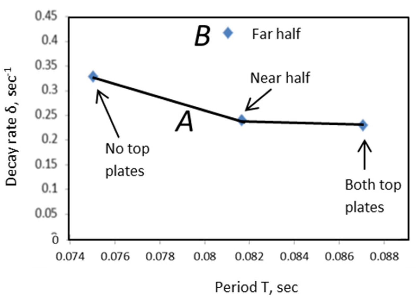
Instead of usual time dependencies, the detection of severe damage can be made in the parameter space. With a weak damage or without damage, the parameters follow a smooth line A in the parameter space. In contrast, a strong damage appears far from the smooth line, as shown in Figure 34 (point B).
A similar behavior was observed in experiments with a plastic rod [29] (for severe damage, the frequency decreased by 3%, but the decay rate increased twofold). In this case, parameter space can also be used to advantage. The current experiment, along with the experiment with the rod, demonstrates the potential for recognizing a structural damage in the parameter space.
6. Discussion
All measurements in Section 4 and Section 5 are based entirely on the experimental photographs and videos.
As an additional option, a noise can be added to the simulated oscillations. Other conditions (e.g., weather) can be also modeled by adding images of raindrops, snowflakes, etc. over the image of the ideal grid. Moreover, the simulated motion in principle allows previously recorded signals to be reproduced and re-measured under changed conditions (using different parameters, distances, cameras, etc.).
The severe damage of the plastic model bridge was primarily due to the greater weight at a longer distance from the support.
Noise has a negative effect on the sensitivity, so the magnification works well at relatively high signal-to-noise ratios.
We do not consider the grid beyond the camera resolution; we only consider its displacement (sometimes almost unrecognizable).
7. Conclusion
The sensitivity threshold was calculated analytically and verified in experiments. Two experimental setups are described, deferred and real-time, where we used rectangular and sinusoidal grid profiles. At a short distance of 2.5 m, the sensitivity threshold was approximately 0.1 mm. The threshold was 0.2 mm (with a zoom lens) at longer distances, up to 20 m. The experiments directly confirmed the sub-pixel sensitivity of the moiré measurement, where the measured amplitude was less than one pixel on the screen. The verified proven feature can be applied to measure vibration in various infrastructure objects (bridges, vehicles, buildings) and allows the use of the moiré measurement system in public safety applications.
Author Contributions
Conceptualization, V.S. and Y.Y.; methodology, V.S.; software, V.S.; validation, V.S. and G.H.; formal analysis, V.S.; resources, G.H.; writing—original draft preparation, V.S.; writing—review and editing, V.S.; visualization, V.S.; supervision, G.H.; project administration, G.H.; funding acquisition, G.H. All authors have read and agreed to the published version of the manuscript.
Funding
This research was funded by the National Research Foundation of Korea, grant number NRF2018R1A6A1A03025542.
Data Availability Statement
Dataset available on request from the authors.
Conflicts of Interest
The authors declare no conflicts of interest.
Abbreviations
The following abbreviations are used in this manuscript:
| CCD | Charge-coupled device |
| RAM | Random-access memory |
| FHD | Full high definition |
| FPS | Frames per second |
References
- Amidror, I. The Theory of the Moiré Phenomenon, Volume I: Periodic layers; Publisher: Springer, London, UK, 2009; pp. 1–2, 165–190. [Google Scholar]
- Sciammarella, C.A. Basic optical law in the interpretation of moiré patterns applied to the analysis of strains. Exp. Mech. 1965, 5, 154–160. [Google Scholar] [CrossRef]
- Yokozeki, S.; Kusaka, Y.; Patorski, K. Geometric parameters of moiré fringes. Appl. Opt. 1976, 15, 2223–2227. [Google Scholar] [CrossRef] [PubMed]
- Patorski, K.; Kujawinska, M. ; Handbook of the Moiré Fringe Technique; Publisher: Elsevier, London, UK, 1993; pp. 99–135. [Google Scholar]
- Saveljev, V.; Kim, S.-K.; Kim, J. Moiré effect in displays: tutorial. Opt. Eng. 2018, 57, 030803. [Google Scholar] [CrossRef]
- Creath, K.; Wyant, J.C. Moiré and fringe projection techniques. In Optical Shop Testing, 2nd ed.; Malacara, D., Ed.; John Wiley & Sons: New York, 1992; pp. 653–685. [Google Scholar]
- Kafri, O.; Glatt, I. The Physics of Moiré Metrology; Publisher: Willey and Sons, New York, USA, 1990; pp. i-ii, 1-18, 78-90.
- Saveljev, V. The Geometry of the Moiré Effect in One, Two, and Three Dimensions; Cambridge Scholars: Newcastle upon Tyne, England, 2022. [Google Scholar]
- Oster, G.; Wasserman, M.; Werling, C. Theoretical interpretation of moiré patterns. J. Opt. Soc. Am. 1964, 54, 169–175. [Google Scholar] [CrossRef]
- Sciammarella, C.A. The moiré method - a review. Exp. Mech. 1982, 22, 418–433. [Google Scholar] [CrossRef]
- Theocaris, P.S. Moiré Fringes in Strain Analysis; Pergamon Press: London, 1969. [Google Scholar]
- Bryngdahl, O. Moiré: Formation and interpretation. J. Opt. Soc. Am. 1974, 64, 1287–1294. [Google Scholar] [CrossRef]
- Hutley, M.C.; Hunt, R.; Stevens, R.F.; Savander, P. The moiré magnifier. Pure Appl. Opt.: J. Europ. Opt. Soc. P. A 1994, 3, 133–142. [Google Scholar] [CrossRef]
- Kamal, H.; Volkel, H.; .Alda, J. Properties of moiré magnifiers. Opt. Eng. 1998, 37, 3007–3014. [Google Scholar]
- Saveljev, V.; Kim, S.-K. Simulation and measurement of moiré patterns at finite distance. Opt. Express 2012, 20, 2163–2177. [Google Scholar] [CrossRef]
- Wu, W.-H.; Wu, C.; Chang, C.-C. Double-sided autostereoscopic imaging with moiré approach. Proceedings of Three-Dimensional Systems and Application (3DSA), Osaka, Japan; 2013; p. 130. [Google Scholar]
- Post, D.; Han, B.; Ifju, P. High Sensitivity Moiré: Experimental Analysis for Mechanics and Materials; Springer: New York, 1994. [Google Scholar]
- Kafri, O.; Band, Y.B.; Chin, T.; Heller, D.F.; Walling, J.C. Real-time moiré vibration analysis of diffusive objects. Appl. Opt. 1985, Vol. 24, No. 2, pp. 240-242.
- Asundi, A. Computer aided moiré methods. Opt. Lasers Eng. 1993, 18, 213–238. [Google Scholar] [CrossRef]
- Shi, W.; Zhang, Q.; Xie, H.; He, W. A binocular vision-based 3d sampling moiré method for complex shape measurement. App. Sci. 2021, 11, 5175. [Google Scholar] [CrossRef]
- Li, C.; Liu, Z.; Xie, H.; Wu, D. Novel 3D SEM moiré method for micro height measurement. Opt.Express 2013, 21, 15734–15746. [Google Scholar] [CrossRef] [PubMed]
- Chiang, C. Moiré topography. Appl. Opt. 1975, 14, 177–179. [Google Scholar] [CrossRef]
- Yokozeki, S.; Mihara, S. Moiré interferometry. Appl. Opt. 1979, 18 1275-1280.
- Wenzel, K.; Abraham, G.; Tamas, P.; Urbin, A. Measurement of distortion using the moiré interferometry. Optics 2015, 4, 14–17. [Google Scholar] [CrossRef]
- Chiang, F.P. Moiré methods in strain analysis. Exp. Mech. 1979, 19, 290–308. [Google Scholar] [CrossRef]
- Stricker, J.; Politch, J. Holographic moiré deflectometry - a method for stiff density field analysis. Appl. Phys. Lett. 1984, 44, 723–725. [Google Scholar] [CrossRef]
- Wen, H.; Liu, Z.; Li, C.; He, X.; Rong, J.; Huang, X.; Xie, H. Centrosymmetric 3D deformation measurement using grid method with a single-camera. Exp. Mech. 2017, 57, 537–546. [Google Scholar] [CrossRef]
- Rasouli, S.; Shahmohammadi, M. Portable and long-range displacement and vibration sensor that chases moving moiré fringes using the three-point intensity detection method. OSA Contin. 2018, 1, 1012–1024. [Google Scholar] [CrossRef]
- Saveljev, V.; Son, J.-Y.; Lee, H.; Heo, G. Non-contact measurement of vibrations using deferred moiré patterns. Adv. Mech. Eng. 2022, 15, 1–11. [Google Scholar] [CrossRef]
- Saveljev, V.; Son, J.-Y.; Heo, G. Using deferred moiré method for real-rime measurements. In Proceedings of the Korean Society of Civil Engineers Convention, Conference & Civil Expo, Busan, Korea, 20 October 2022; pp. 7–8. [Google Scholar]
- Yao, Jun; Chen. Jubing. Research on the sensitivity of projection moiré system considering its variety in space. Opt. Lasers Eng. 2018, 110, 1–6. [CrossRef]
- Shin, S.; Sohn, H.-J.; Kang, D.-W. Sensitivity analysis of moiré phenomena under process window variation. In Digest of Tech Papers of International Conference on Display Technology, Hefei, China, 2024, Volume 55, Issue S1, pp. 477-480.
- Du, H.; Wang, J.; Zhao, H.; Jia, P. Calibration of the high sensitivity shadow moiré system using random phase-shifting technique. Opt. Lasers Eng. 2014, 63, 70–75. [Google Scholar] [CrossRef]
- Saveljev, V.; Kim, S.-K. Probability of the moiré effect in barrier and lenticular autostereoscopic 3D displays. Opt.Express 2015, 23, 25597–25607. [Google Scholar] [CrossRef] [PubMed]
- Aggarwal, D.; Narula, R.; Ghosh, S. Moiré fractals in twisted graphene layers. Phys. Rev. B 2024, 109, 125302. [Google Scholar] [CrossRef]
- Voss, H.U.; Ballon, D.J. Moiré patterns of space-filling curves. Phys. Rev. Research 2024, 6, L032035. [Google Scholar] [CrossRef]
- Saunoriene, L.; Saunoris, M.; Ragulskis, M. Image hiding in stochastic geometric moiré gratings. Mathematics 2023, 11, 1763. [Google Scholar] [CrossRef]
- Daemi, M.H.; Rasouli, S. Investigating the dynamic behavior of thermal distortions of the wavefront in a high-power thin-disk laser using the moiré technique. Opt. Lett. 2020, 45, 4567–4570. [Google Scholar] [CrossRef]
- Rasouli, S.; Yeganeh, M. Formulation of the moiré patterns formed by superimposing of gratings consisting topological defects: moiré technique as a tool in singular optics detections. J. Opt. 2015, 17, 105604. [Google Scholar] [CrossRef]
- Yeganeh, M.; Rasouli, S.; Dashti, M.; Slussarenko, S.; Santamato, E.; Karimi, E. Reconstructing the Poynting vector skew angle and wave-front of optical vortex beams via two-channel moiré deflectometery. Opt. Lett. 2013, 38, 887–889. [Google Scholar] [CrossRef]
- Wu, W.-H.; Wu, C.; Chang, C.-C. Double-sided autostereoscopic imaging with moiré approach. In Proceedings of the Three-Dimensional Systems and Application (3DSA), Osaka, Japan; 2013; p. 130. [Google Scholar]
- Saveljev, V.; Kim, S.-K. Three-dimensional moiré display. J. Soc. Inf. Disp. 2015, 22, 482–486. [Google Scholar] [CrossRef]
- Mori, S.; Bao, Y. Autostereoscopic display with LCD for viewing a 3-D animation based on the moiré effect. OSA Contin. 2020, 3, 224–235. [Google Scholar] [CrossRef]
- Saveljev, V.; Son, J.-Y.; Heo, G. Simulation of mechanical displacement for the moiré sensor, presented at Korean Society of Civil Engineers Convention, Conference & Civil Expo, Yeosu, Korea, Session J5, 20-Oct-23.
- Saveljev, V.; Heo, G. Experimental confirmation of sub-pixel sensitivity of moiré measurements using a digital camera, presented at Korean Society of Civil Engineers Convention, Conference & Civil Expo, Jeju ICC, Korea, Session H4, 17-Oct-24.
Figure 1.
Moiré effect in similar parallel grids of different periods (difference of 17%).
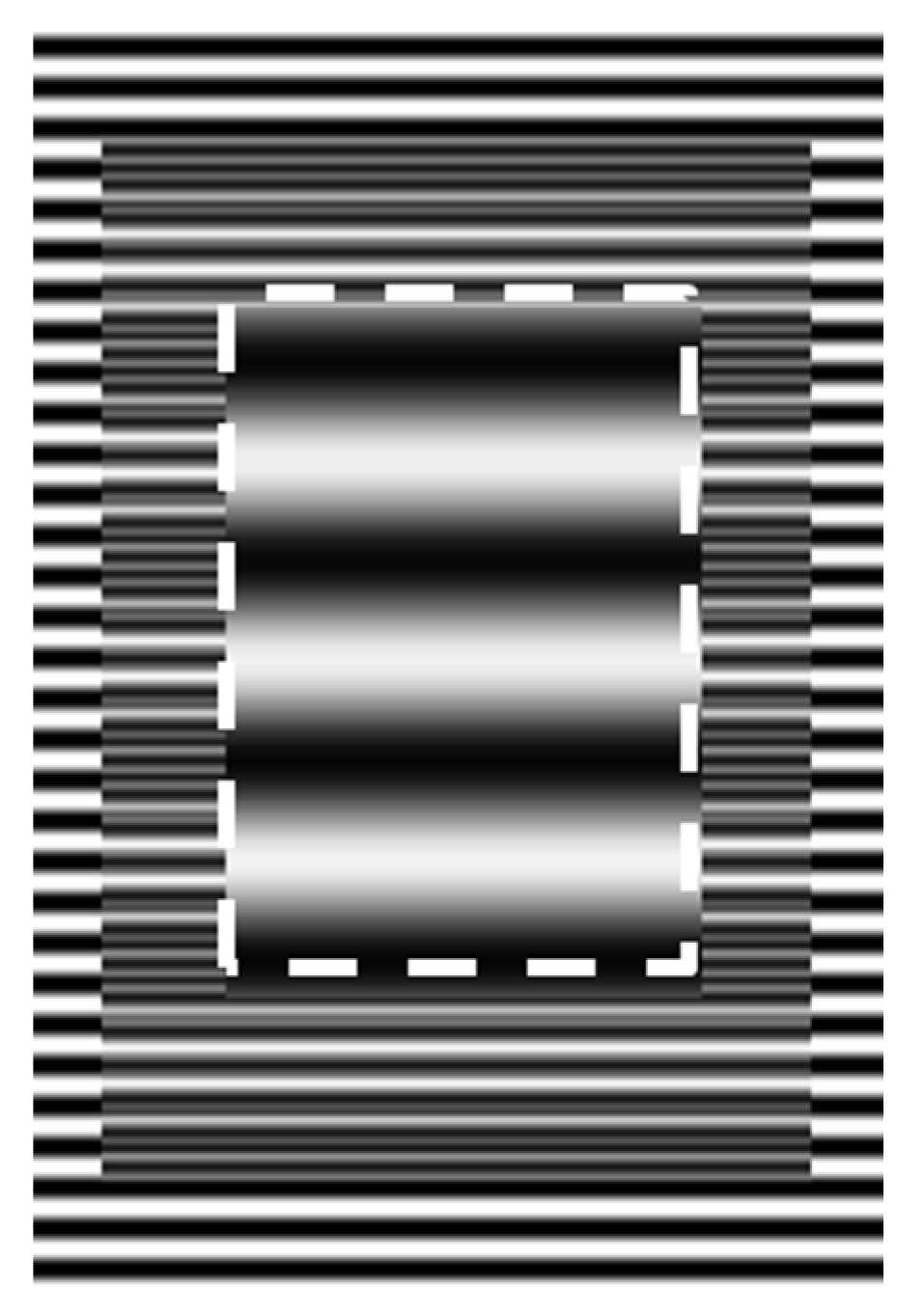
Figure 2.
Sub-pixel sensitivity.
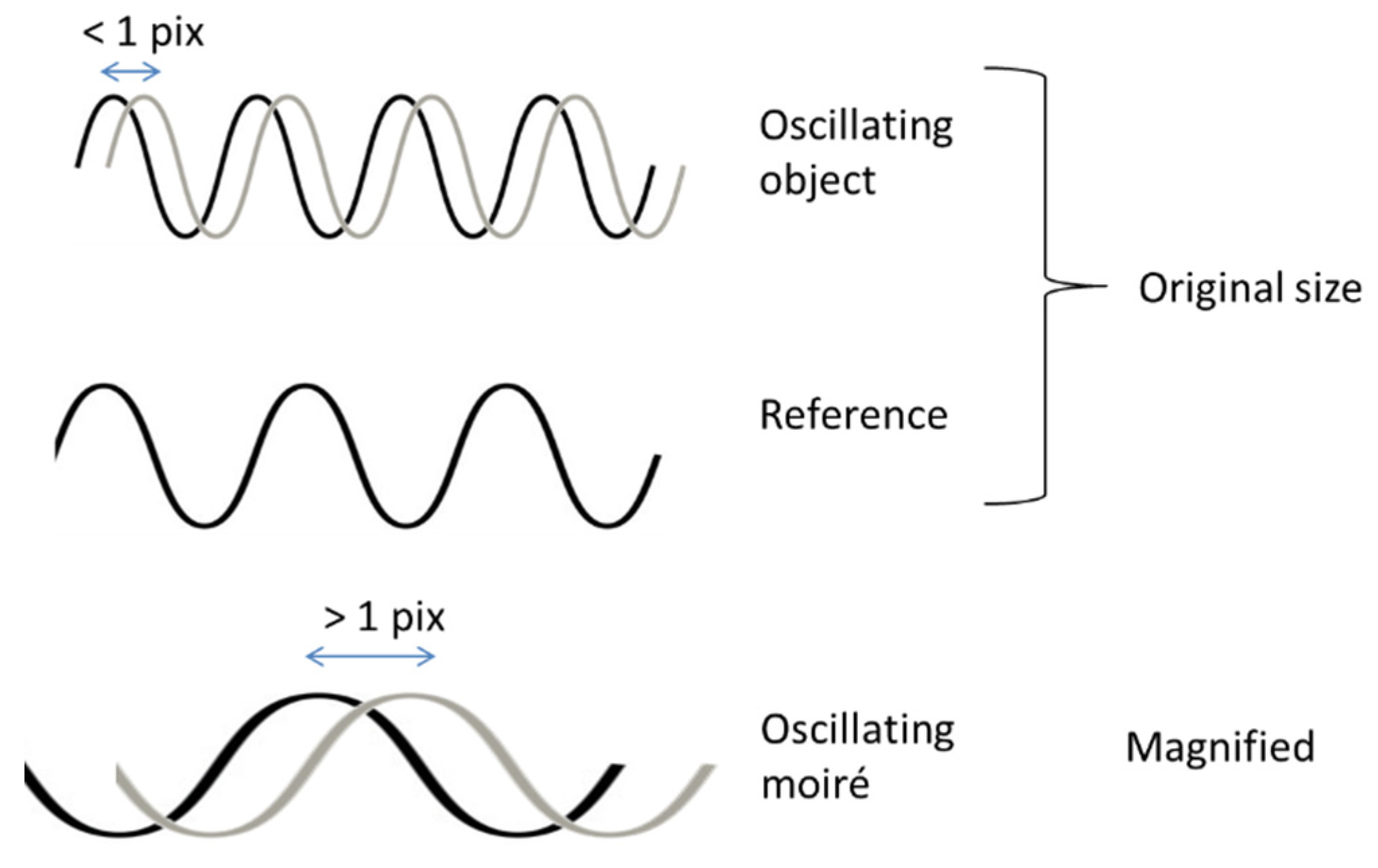
Figure 3.
Sensitivity of digital camera in view of geometrical optics for large L.
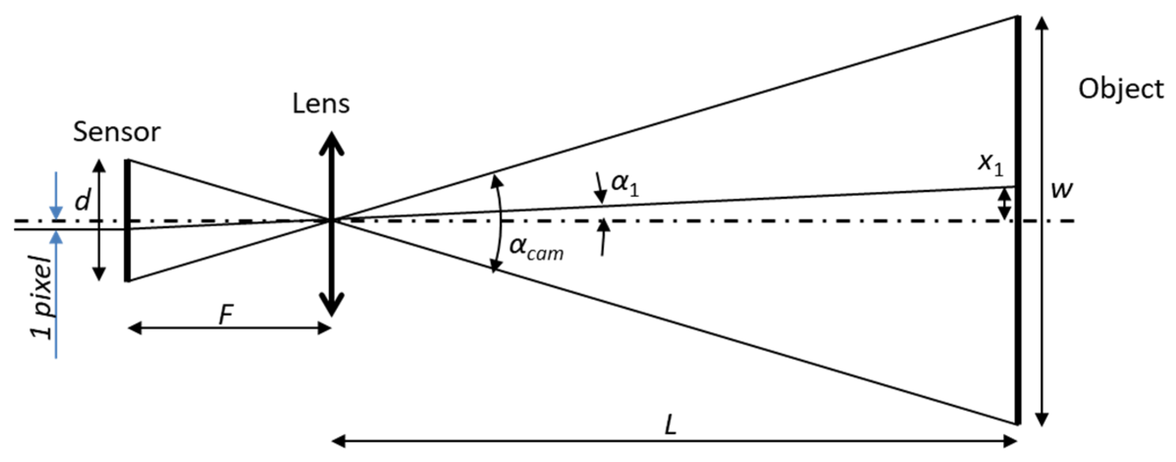
Figure 4.
Blocks of moiré measurement system: ① digital camera on solid ground and ② grid on object.
Figure 4.
Blocks of moiré measurement system: ① digital camera on solid ground and ② grid on object.
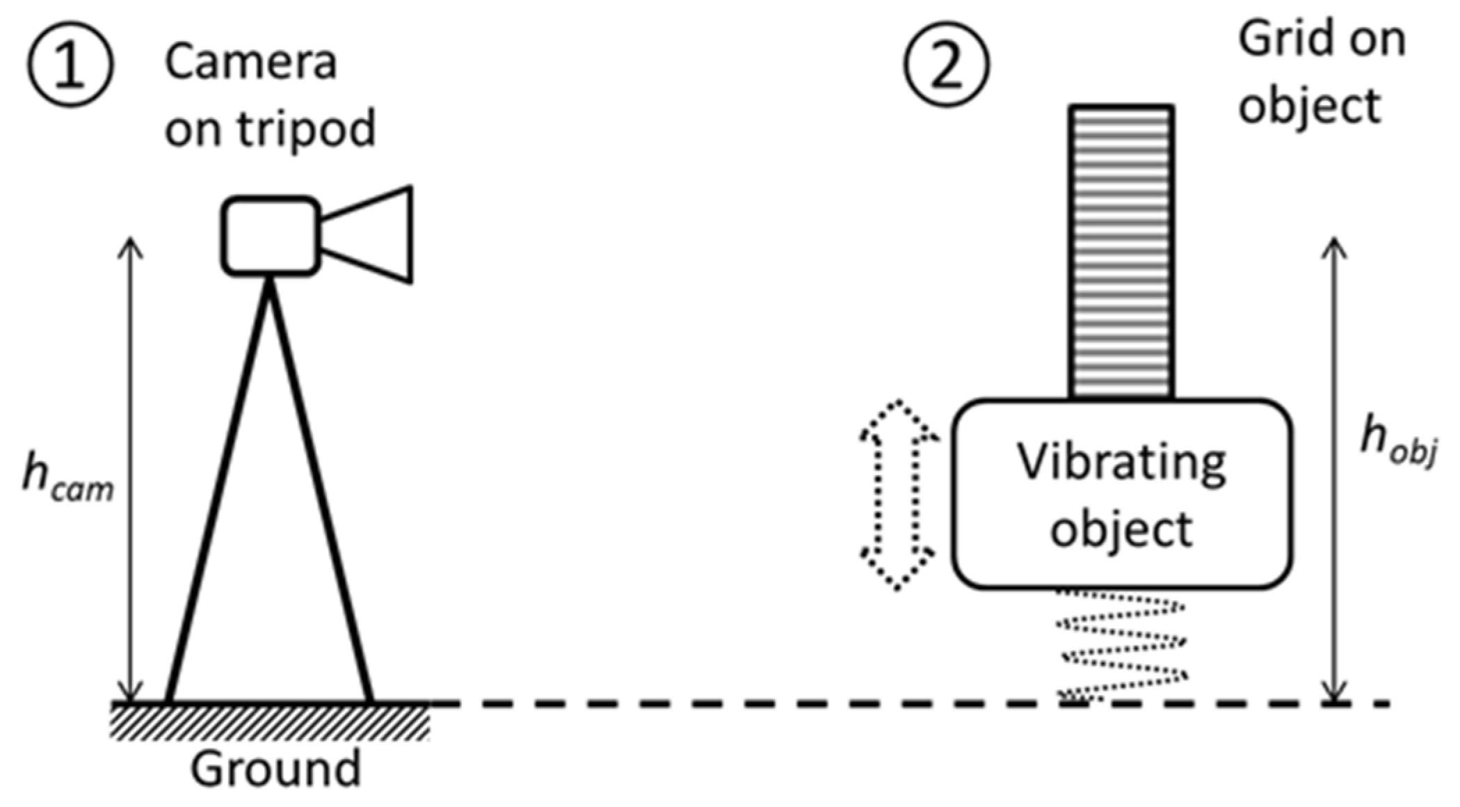
Figure 5.
Moiré patterns in overlapped grids at two moments in time.
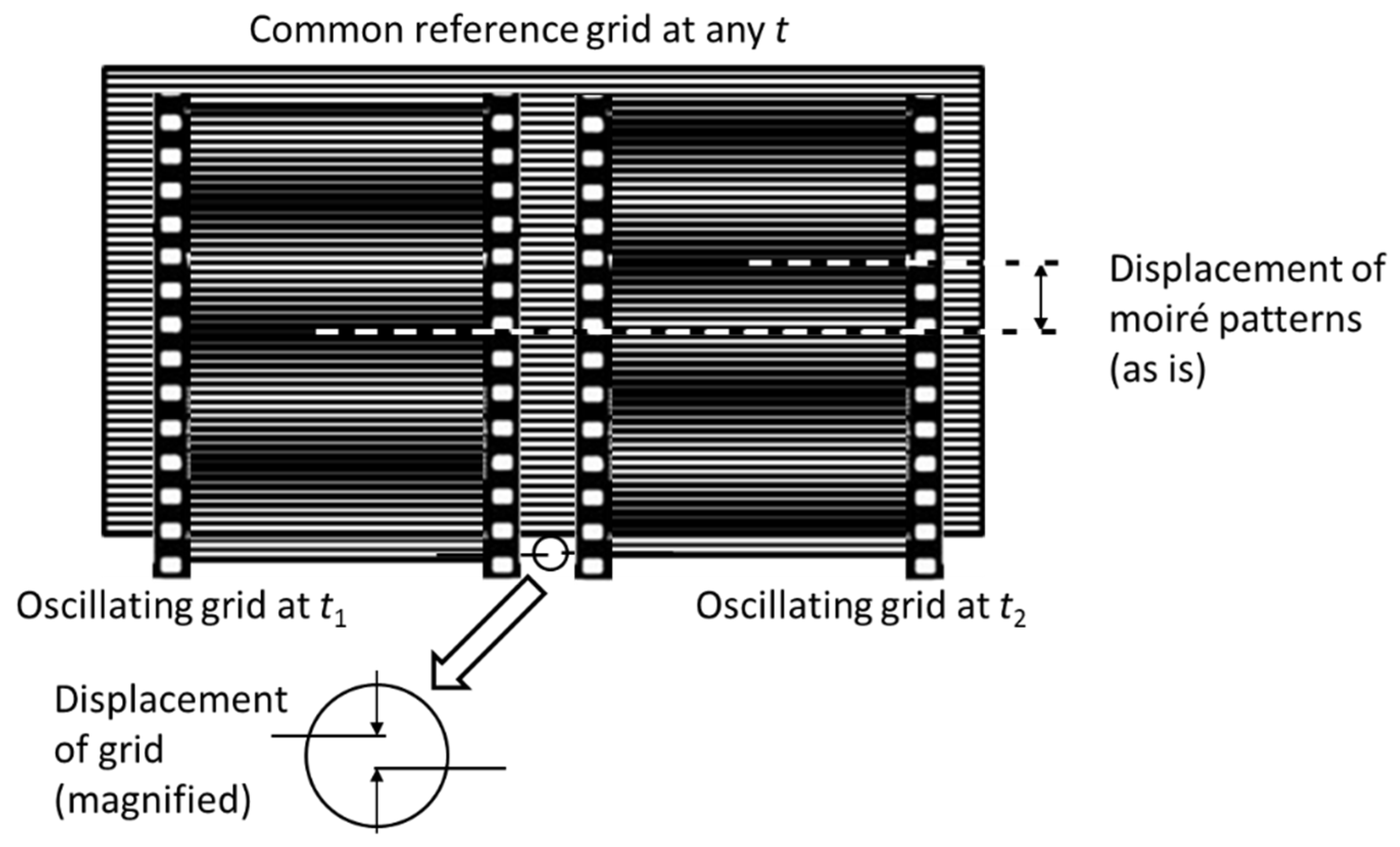
Figure 6.
Experimental setup of the moiré measurement system: (a) deferred, (b) real time.
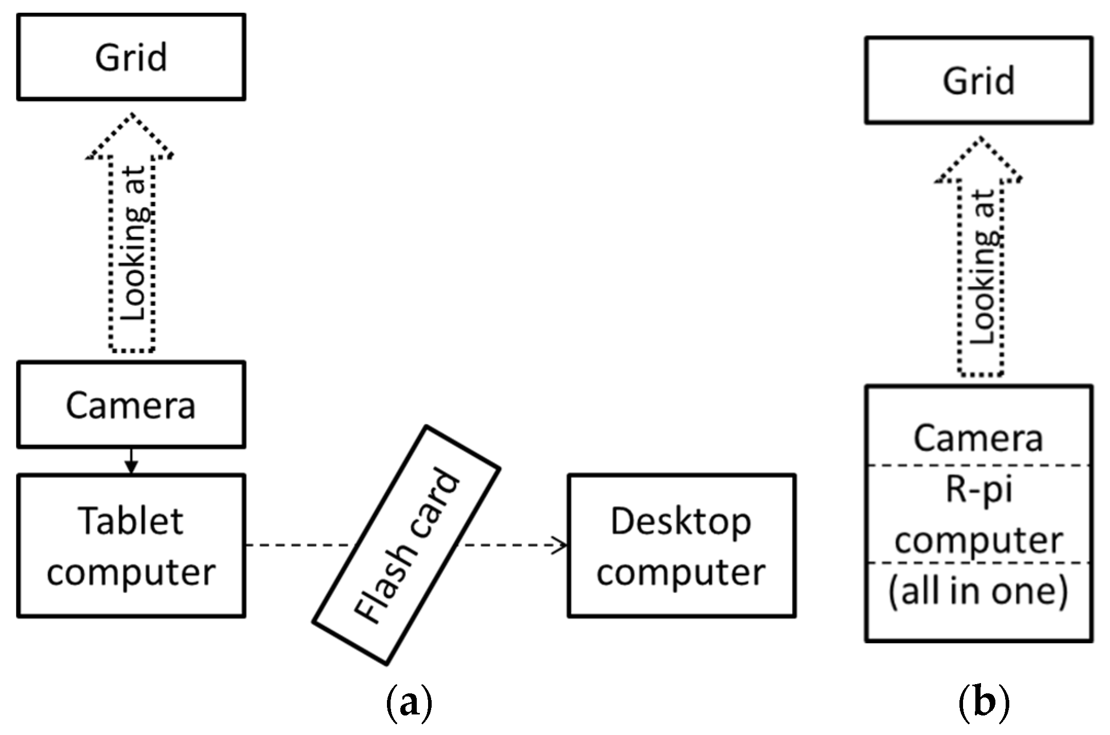
Figure 7.
Moiré measurement system (photographs): (a) deferred version based on the tablet computer and (b) real-time version with controls (keyboard and mouse) based on Raspberry Pi computer.
Figure 7.
Moiré measurement system (photographs): (a) deferred version based on the tablet computer and (b) real-time version with controls (keyboard and mouse) based on Raspberry Pi computer.
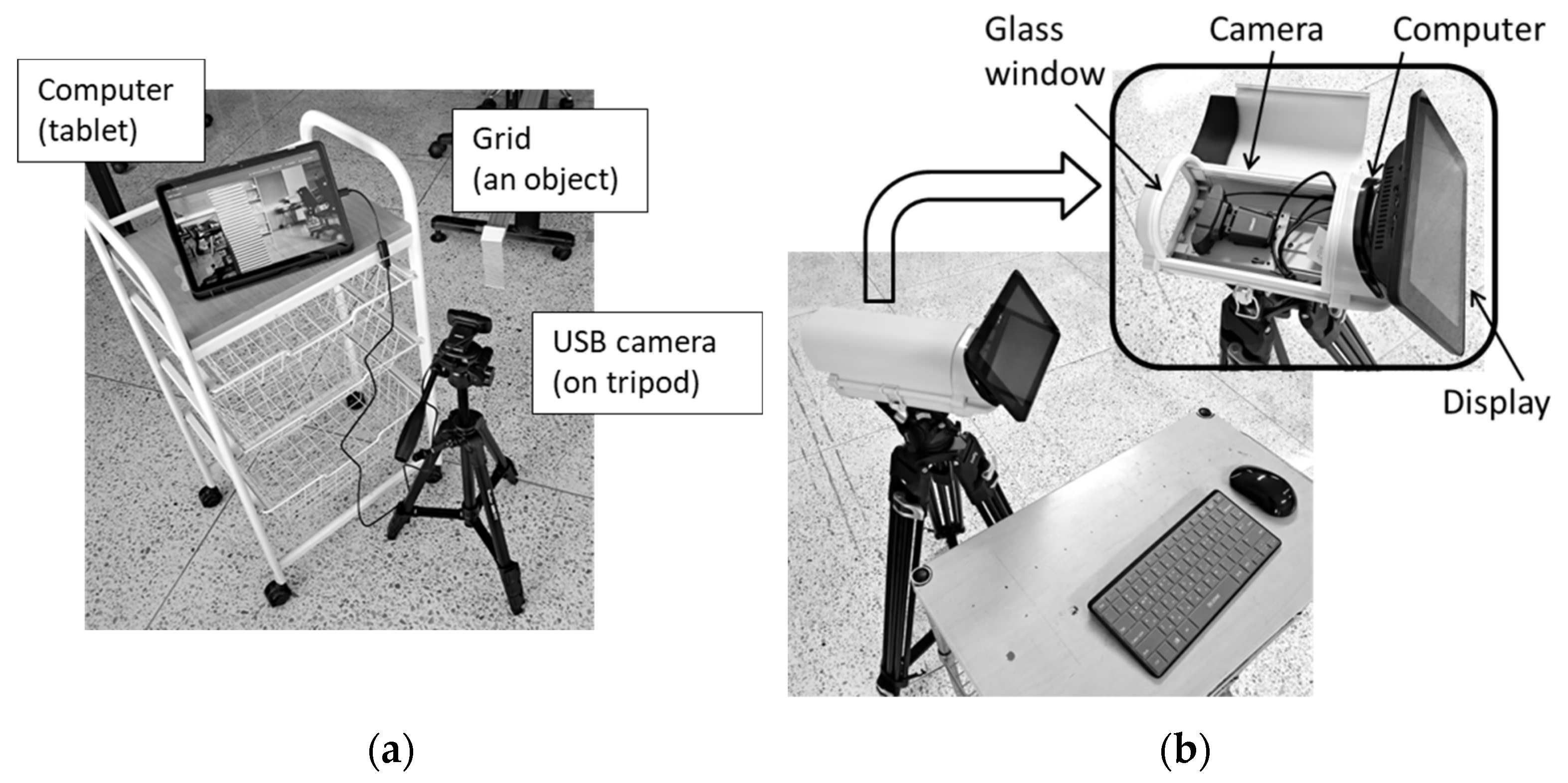
Figure 8.
Computer-generated grid: (a) photograph of entire grid on the monitor screen, (b) magnified part of the screen with numerical values (period and amplitude in pixels and millimeters).
Figure 8.
Computer-generated grid: (a) photograph of entire grid on the monitor screen, (b) magnified part of the screen with numerical values (period and amplitude in pixels and millimeters).
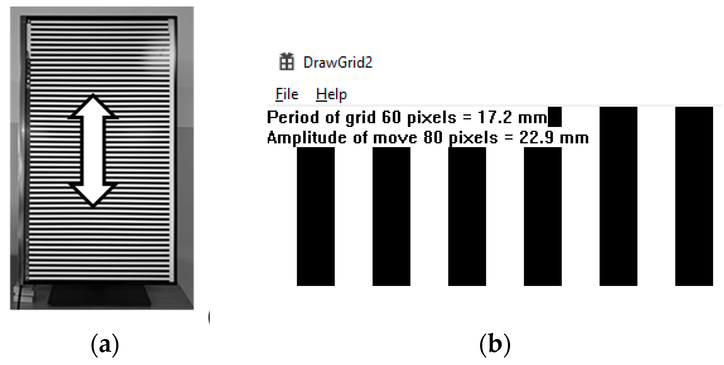
Figure 9.
Simulated displacement of a grid: (a) computer-controlled displacement as a function of time.
Figure 9.
Simulated displacement of a grid: (a) computer-controlled displacement as a function of time.
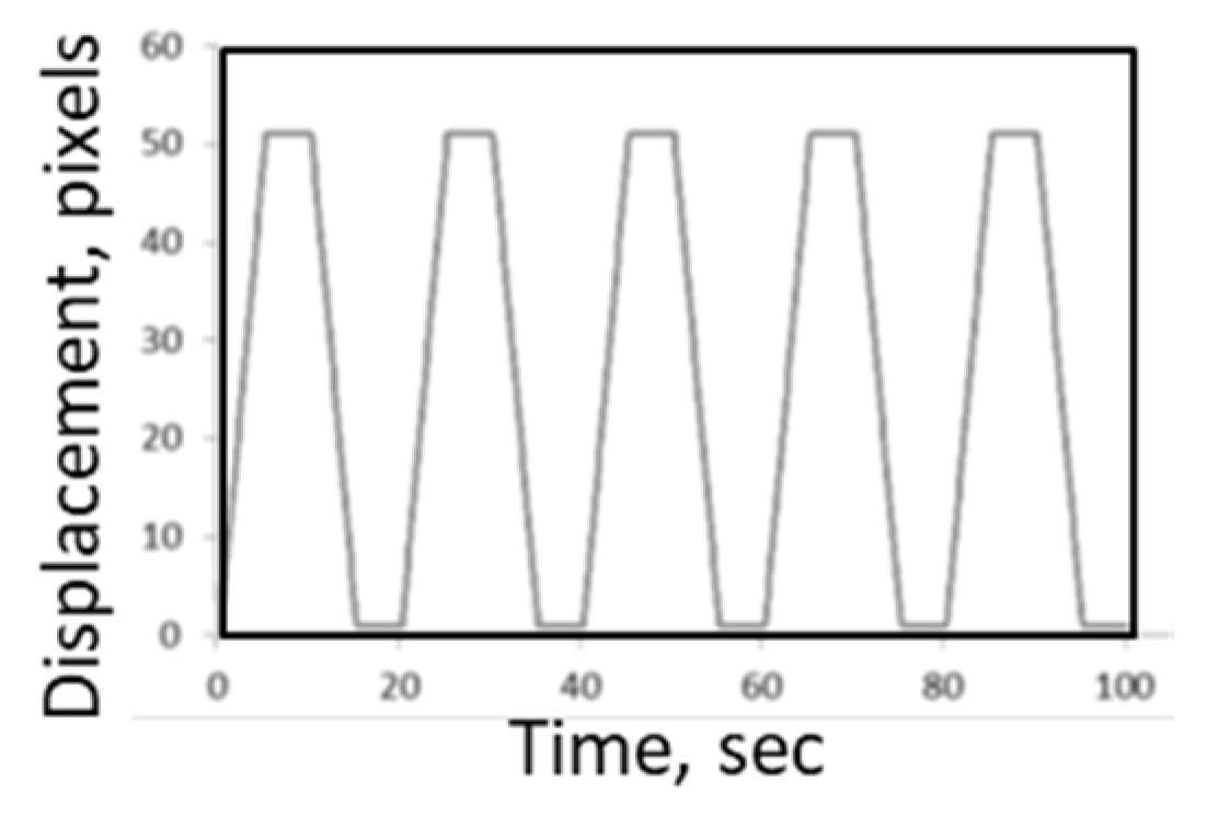
Figure 10.
Measurements of oscillations of a simulated grid motion on the screen (sinusoidal waveform).
Figure 10.
Measurements of oscillations of a simulated grid motion on the screen (sinusoidal waveform).
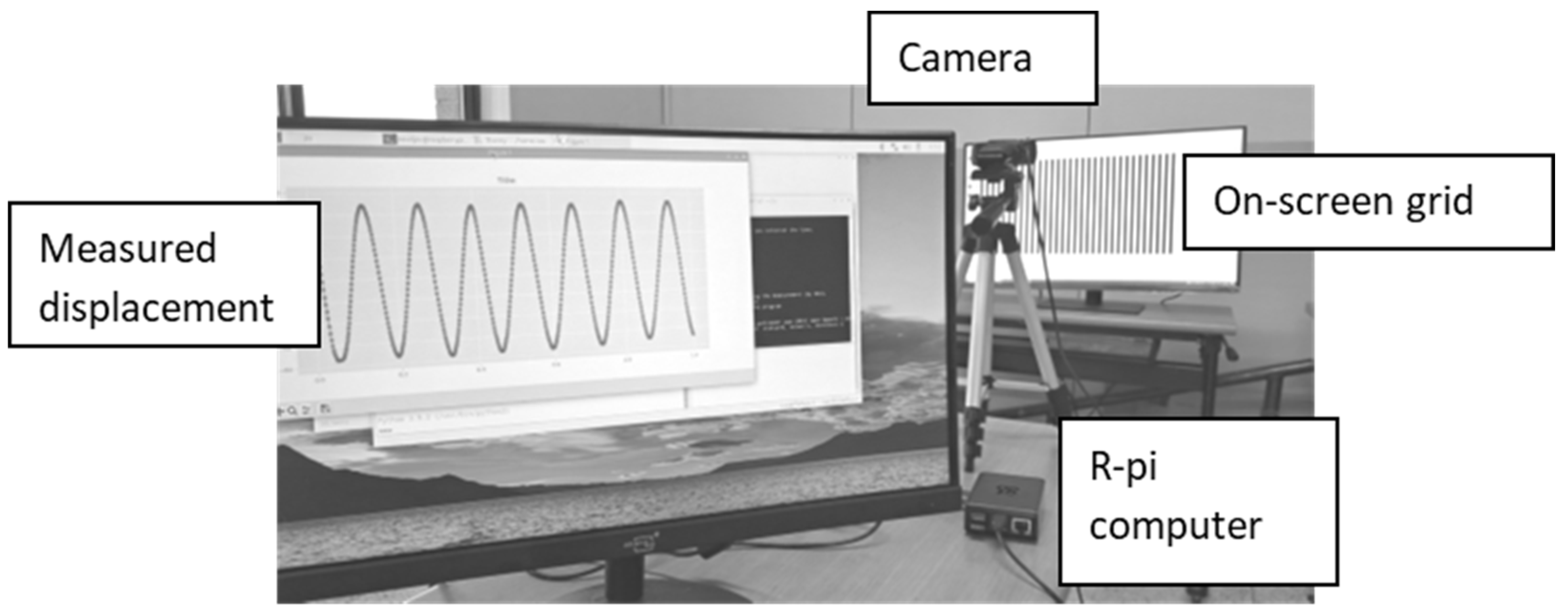
Figure 11.
One frame of the test video 1280x720 (grid with the sinusoidal profile).
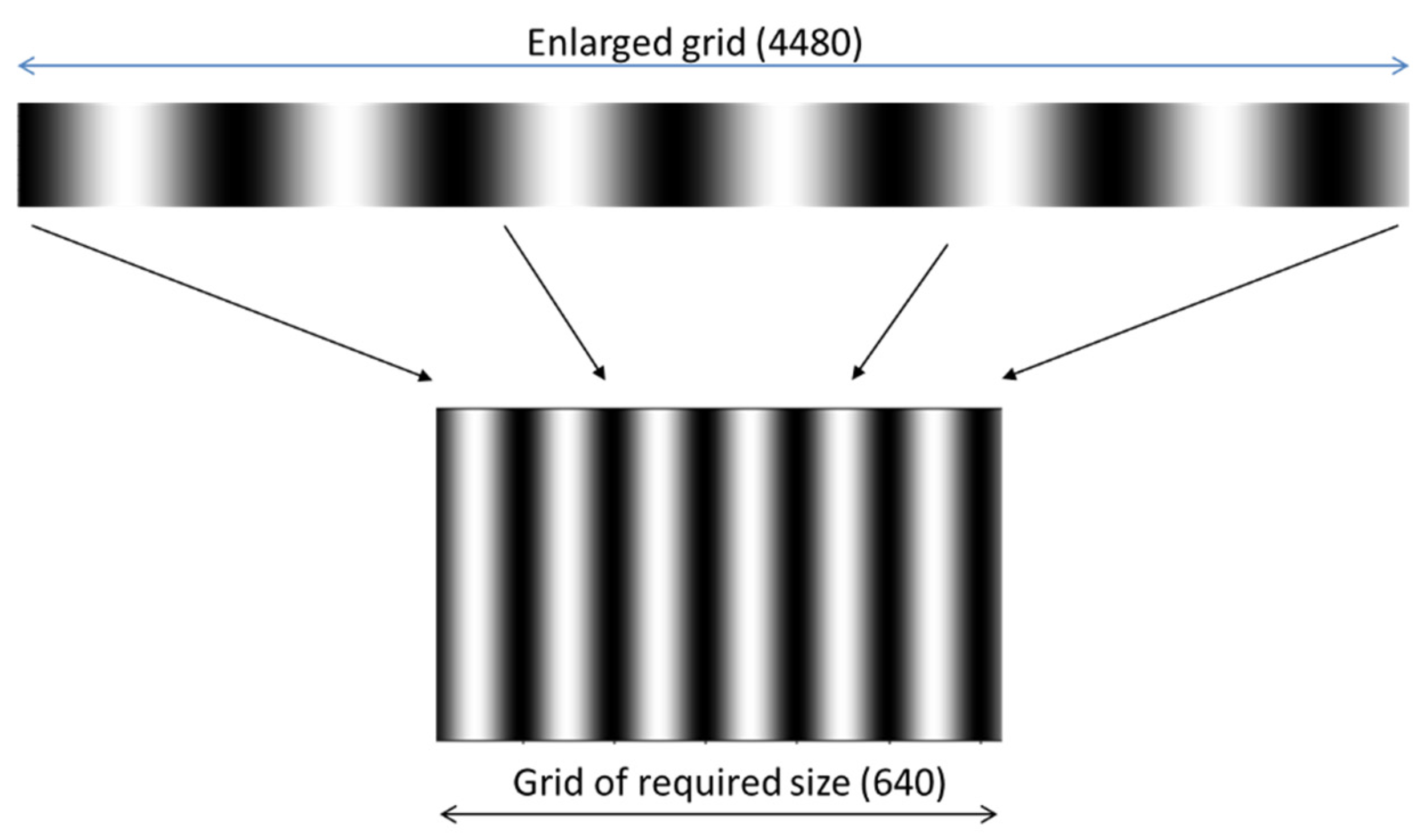
Figure 12.
Experimental setup with mechanical slider.
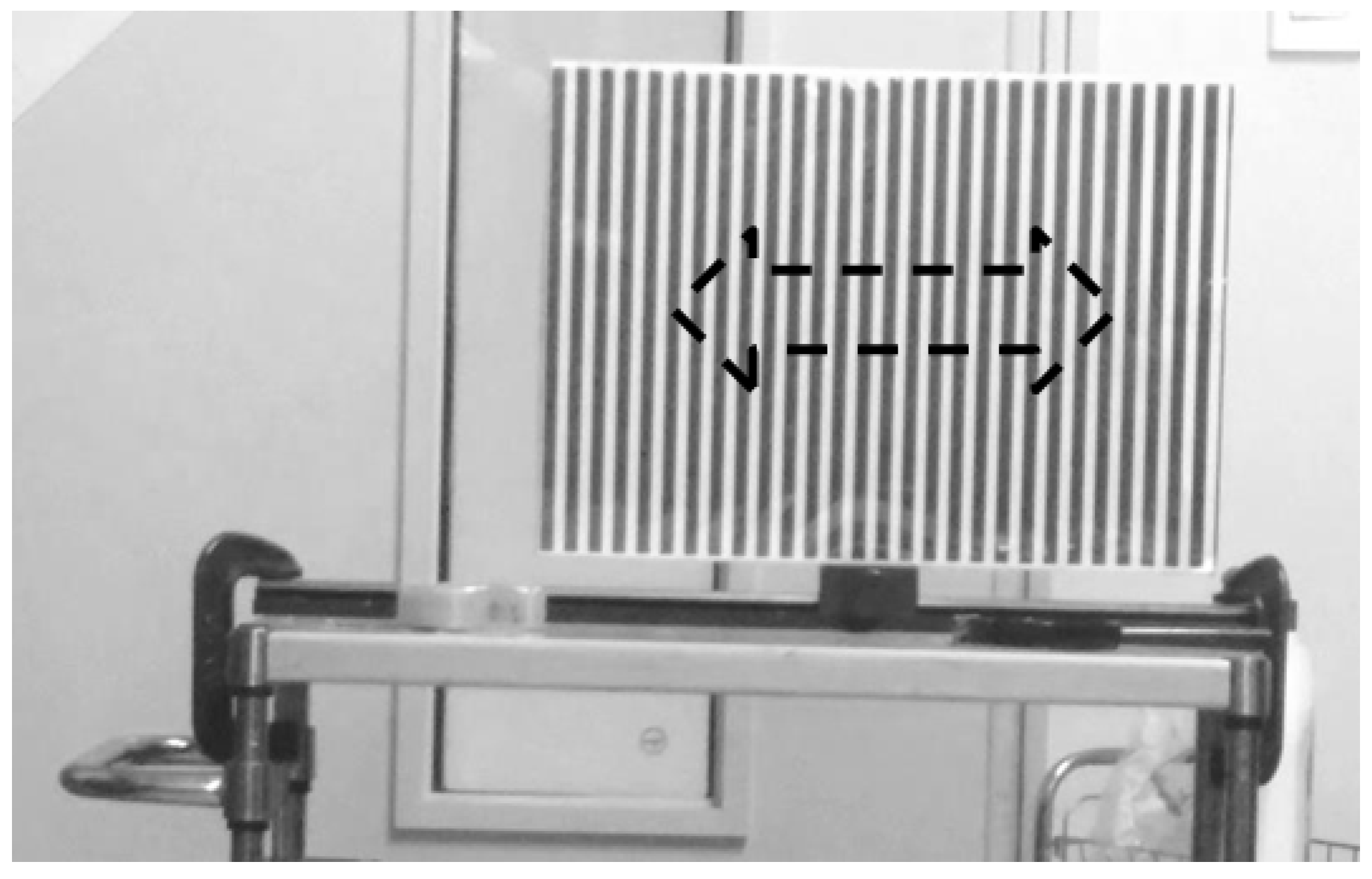
Figure 13.
Measures displacements 0.5, 1, 2, and 5 mm at distances (a) 3 m, (b) 25 m.
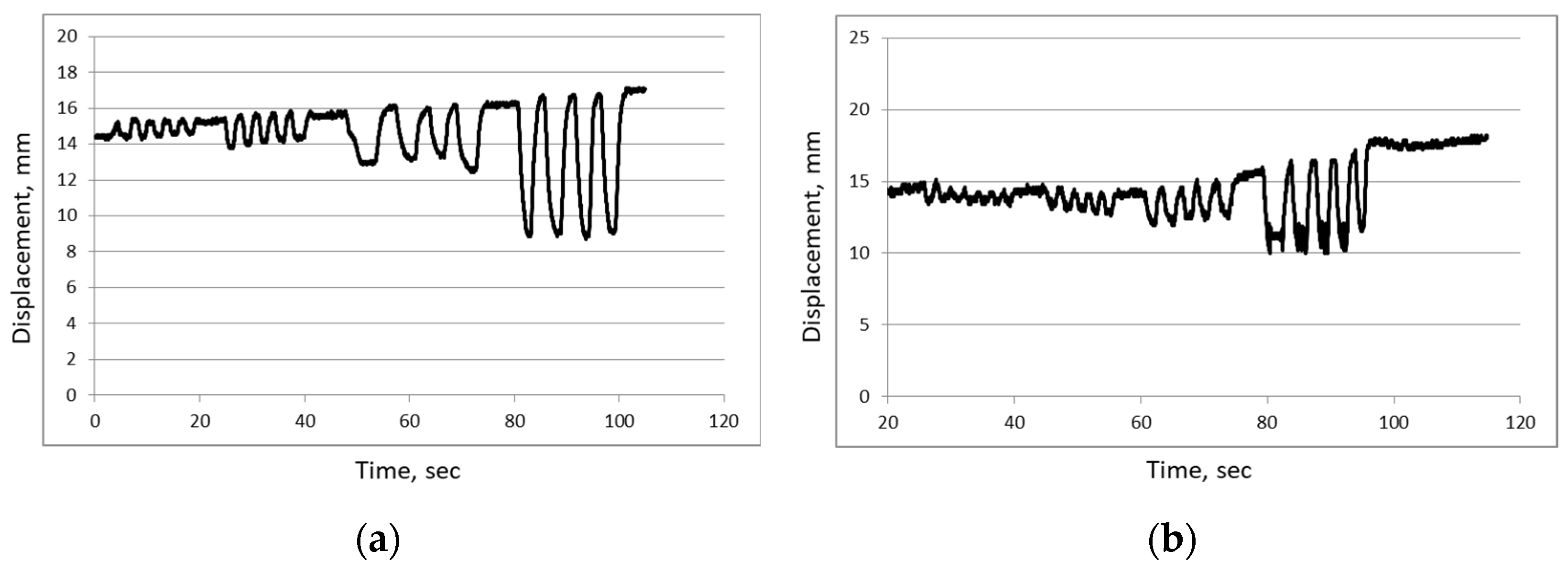
Figure 14.
Grids photographed from different distances. The entire grid (51.5 cm) on the screen is shown by the dashed rectangle. 20 grid lines are shown by the solid rectangle. (a) Grid with pitch 6.7 mm, distance 1.35 m; (b) grid 14 mm, distance 2.8 m; (c) grid 25.8 mm, distance 5.05 m.
Figure 14.
Grids photographed from different distances. The entire grid (51.5 cm) on the screen is shown by the dashed rectangle. 20 grid lines are shown by the solid rectangle. (a) Grid with pitch 6.7 mm, distance 1.35 m; (b) grid 14 mm, distance 2.8 m; (c) grid 25.8 mm, distance 5.05 m.
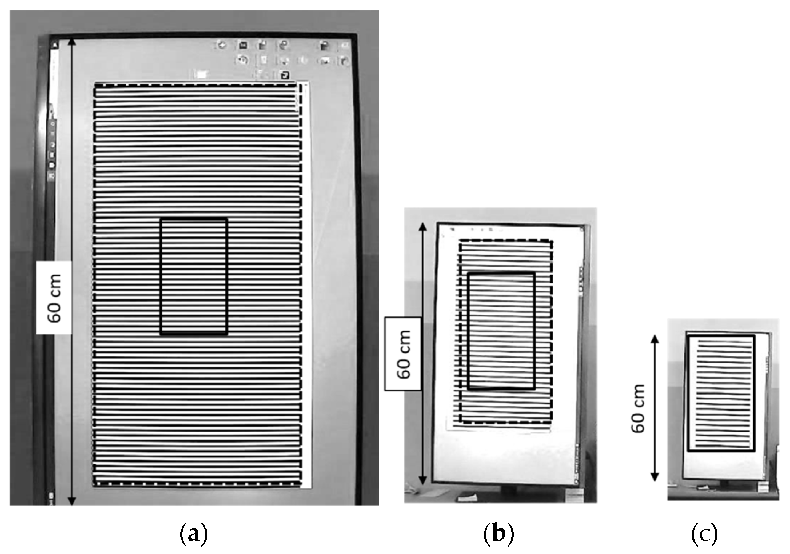
Figure 15.
Measurements of simulated vibrations of 0.5, 1, and 2 pixels.
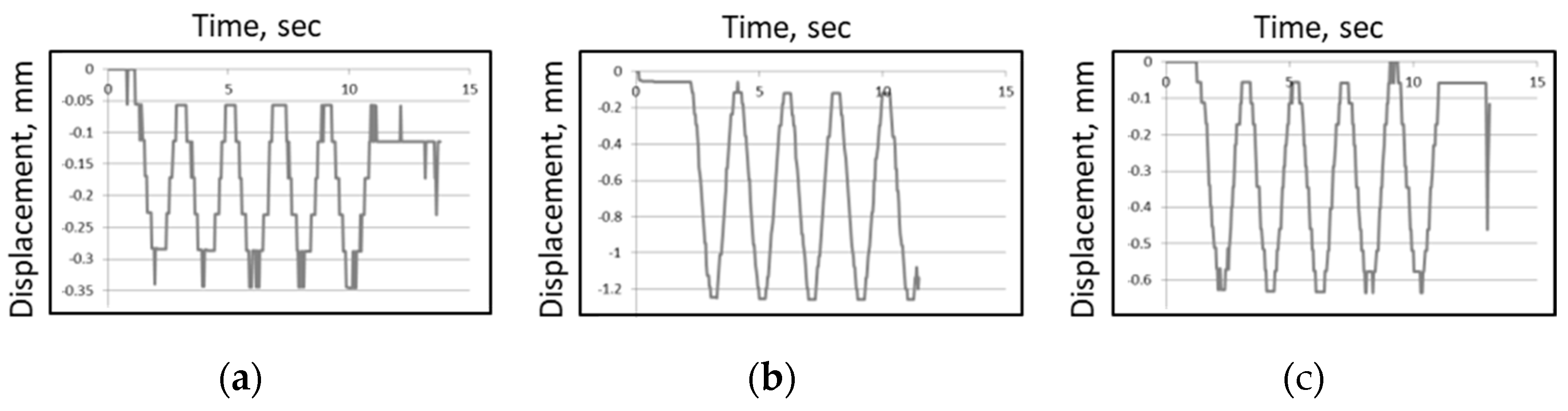
Figure 16.
Vibration mode of the model bridge at 2.9 Hz.
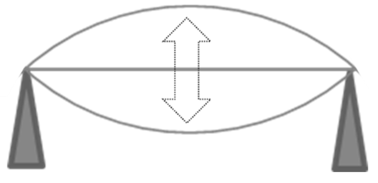
Figure 17.
Measurement system on the model bridge.
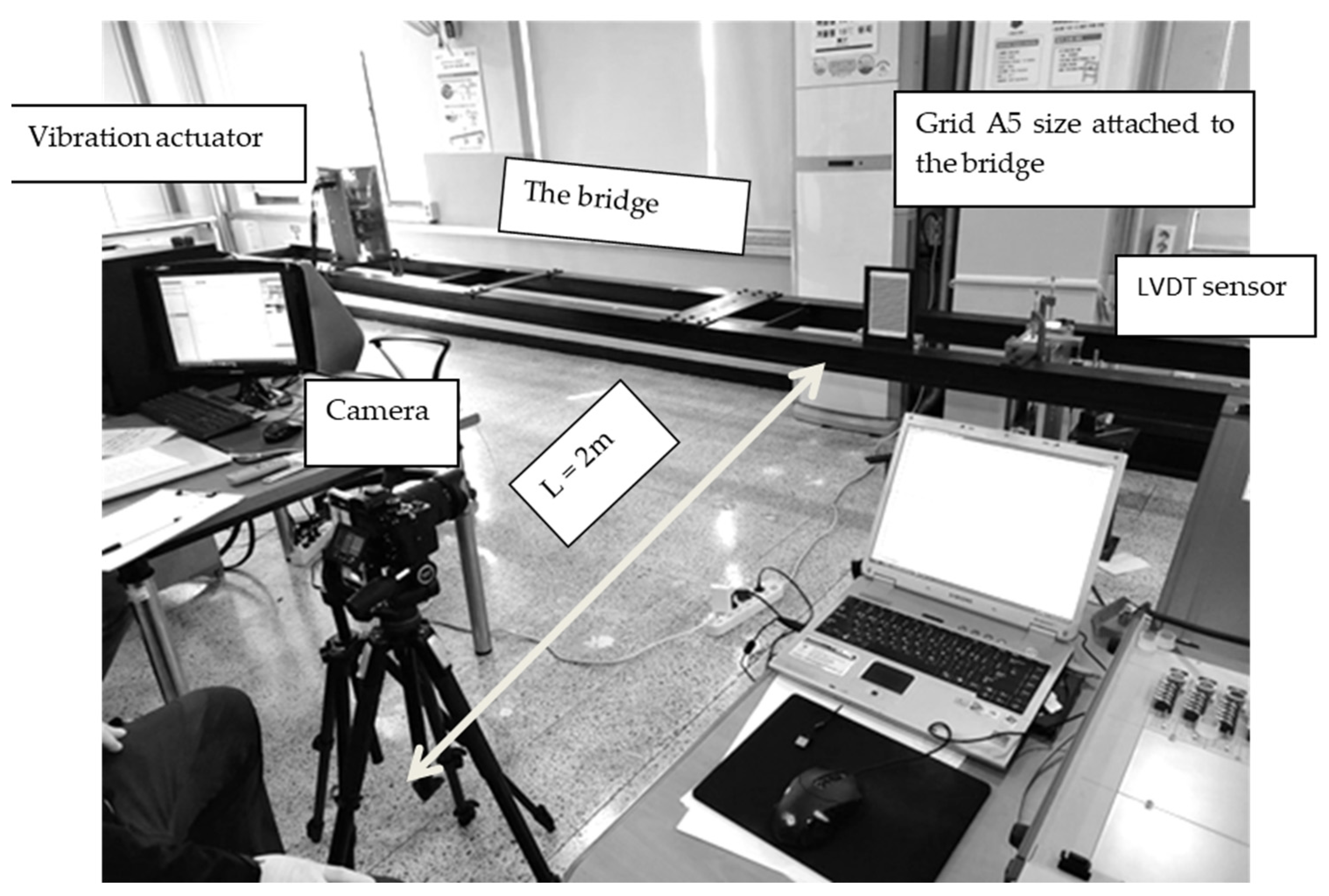
Figure 18.
Measured displacement signal: moiré method (dotted line) and LVDT sensor (solid line).
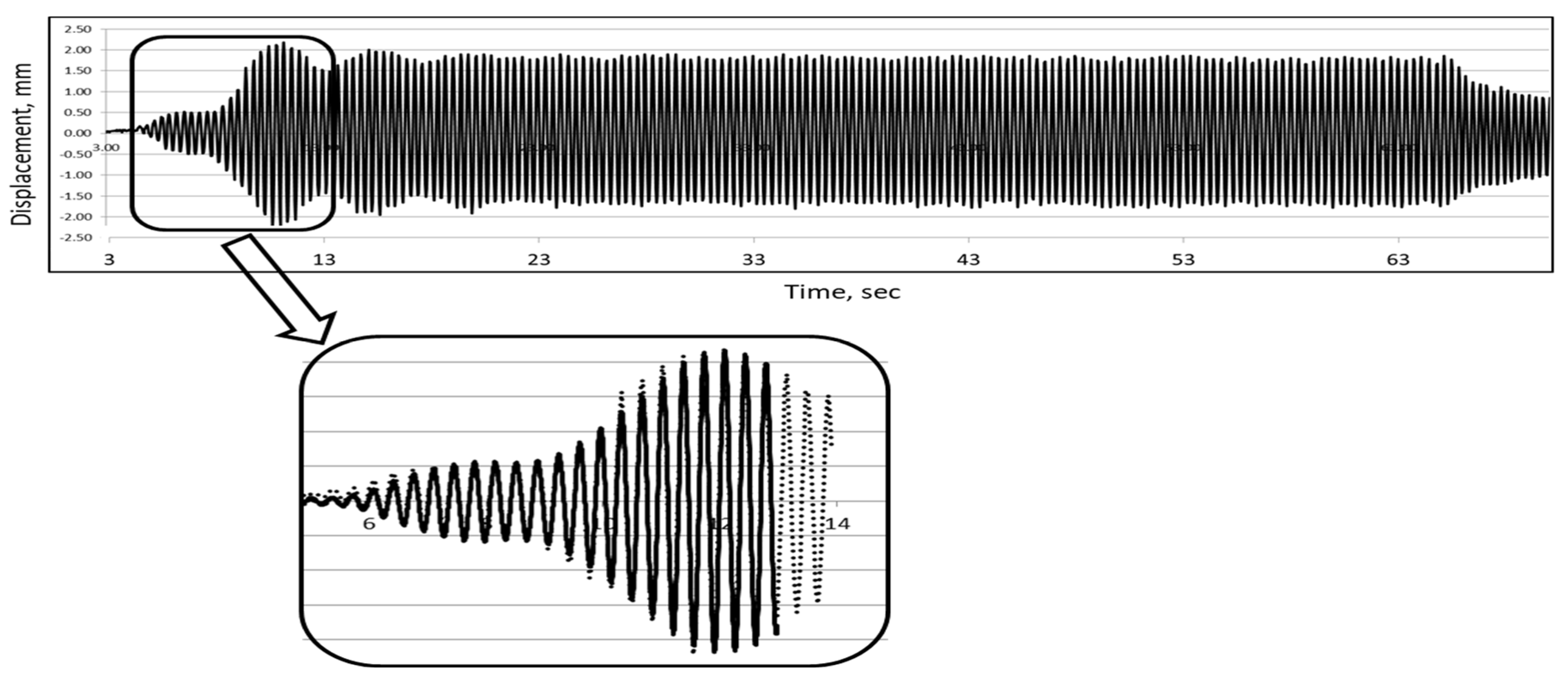
Figure 19.
Comparison of the amplitude of vibration measured by two methods.
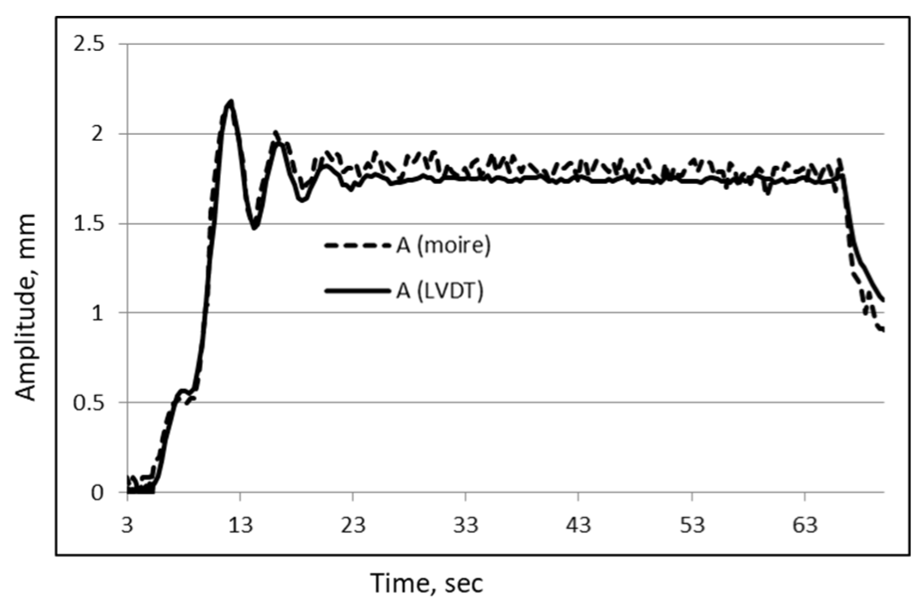
Figure 20.
Vibration machine JINN.
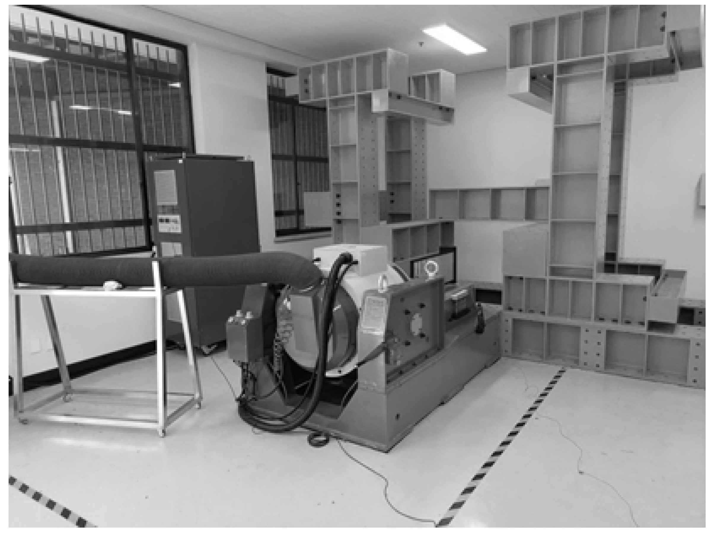
Figure 21.
Moiré measurements on the vibration machine.
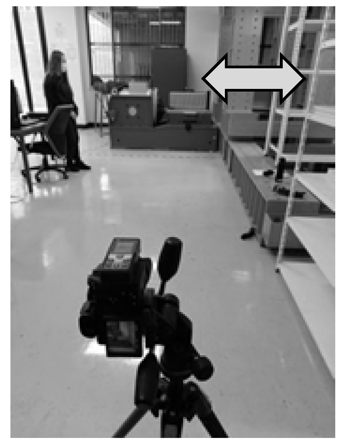
Figure 22.
Measured displacement.
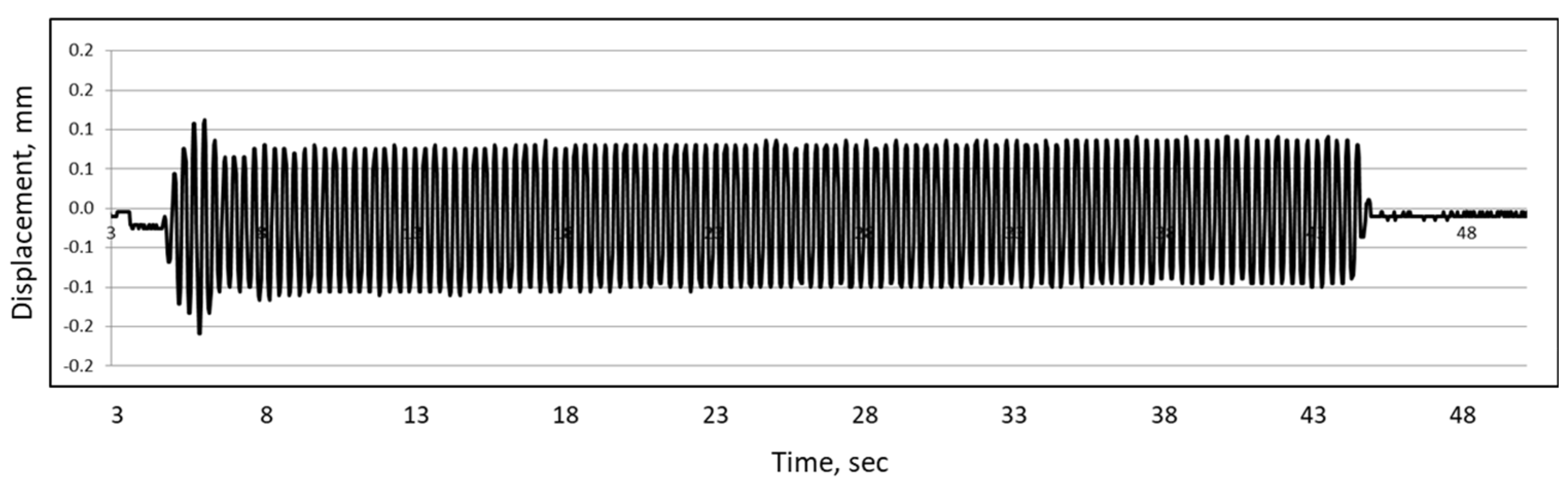
Figure 23.
Measured amplitude: (a) moiré method, (b) machine record.
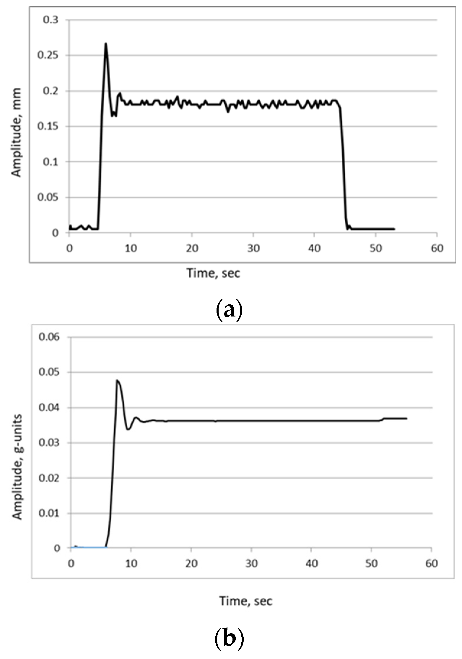
Figure 24.
Short pedestrian bridge 1 with a grid in the middle.
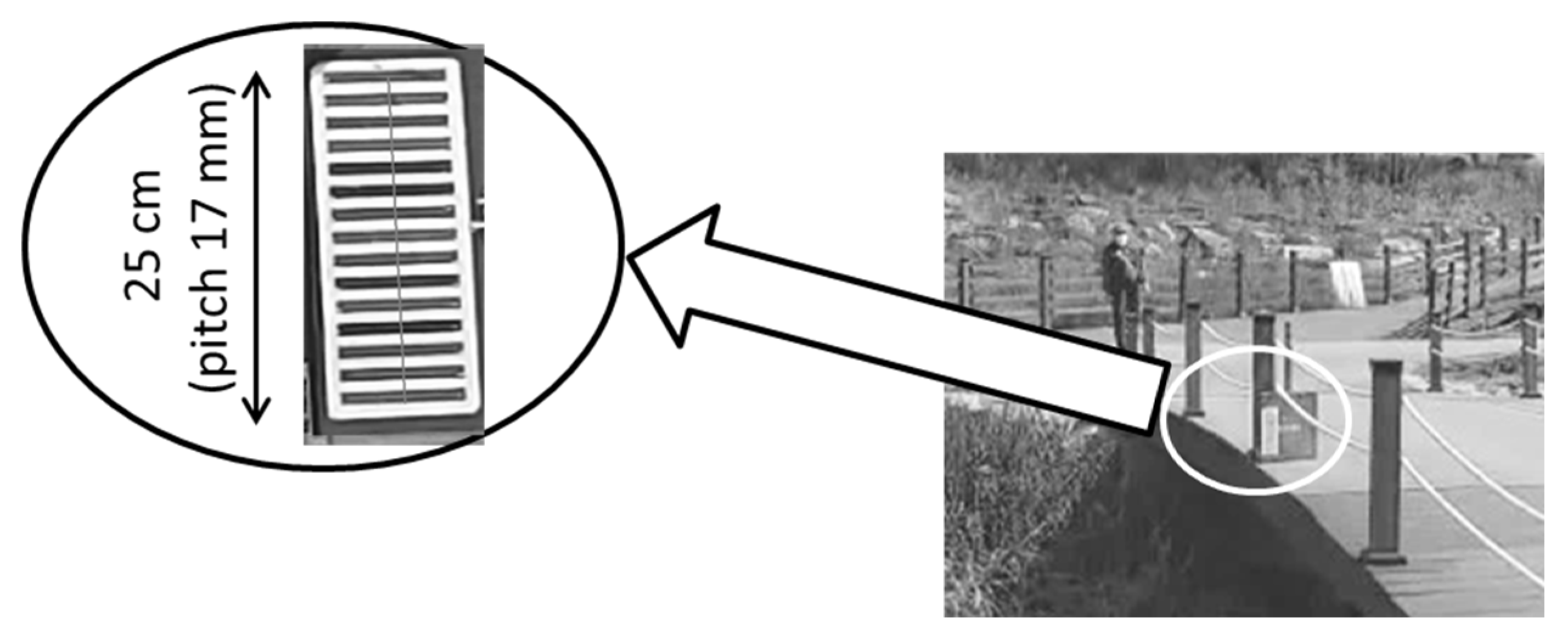
Figure 25.
Example of moiré patterns in measurements (short bridge 1): (a) grid profile as is, (b) smoothed profile, (c) generated grid and (d) moiré patterns.
Figure 25.
Example of moiré patterns in measurements (short bridge 1): (a) grid profile as is, (b) smoothed profile, (c) generated grid and (d) moiré patterns.

Figure 26.
Deflection in a short pedestrian bridge with moving people: (a) walking, (b) running, and (c) cycling.
Figure 26.
Deflection in a short pedestrian bridge with moving people: (a) walking, (b) running, and (c) cycling.

Figure 27.
The grid at a long pedestrian bridge 2 (as seen in camera); the measurement axis is shown by a thin vertical line.
Figure 27.
The grid at a long pedestrian bridge 2 (as seen in camera); the measurement axis is shown by a thin vertical line.
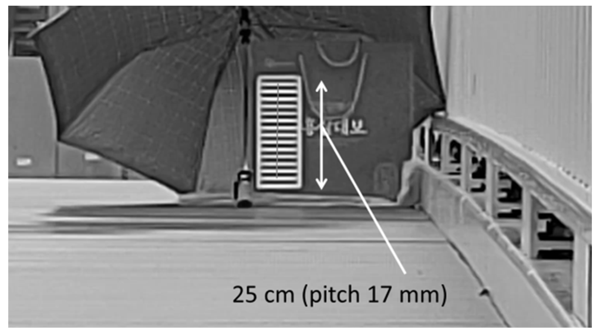
Figure 28.
Measured deflection in a longer bridge 2 with moving people: (a) walking, (b) running.
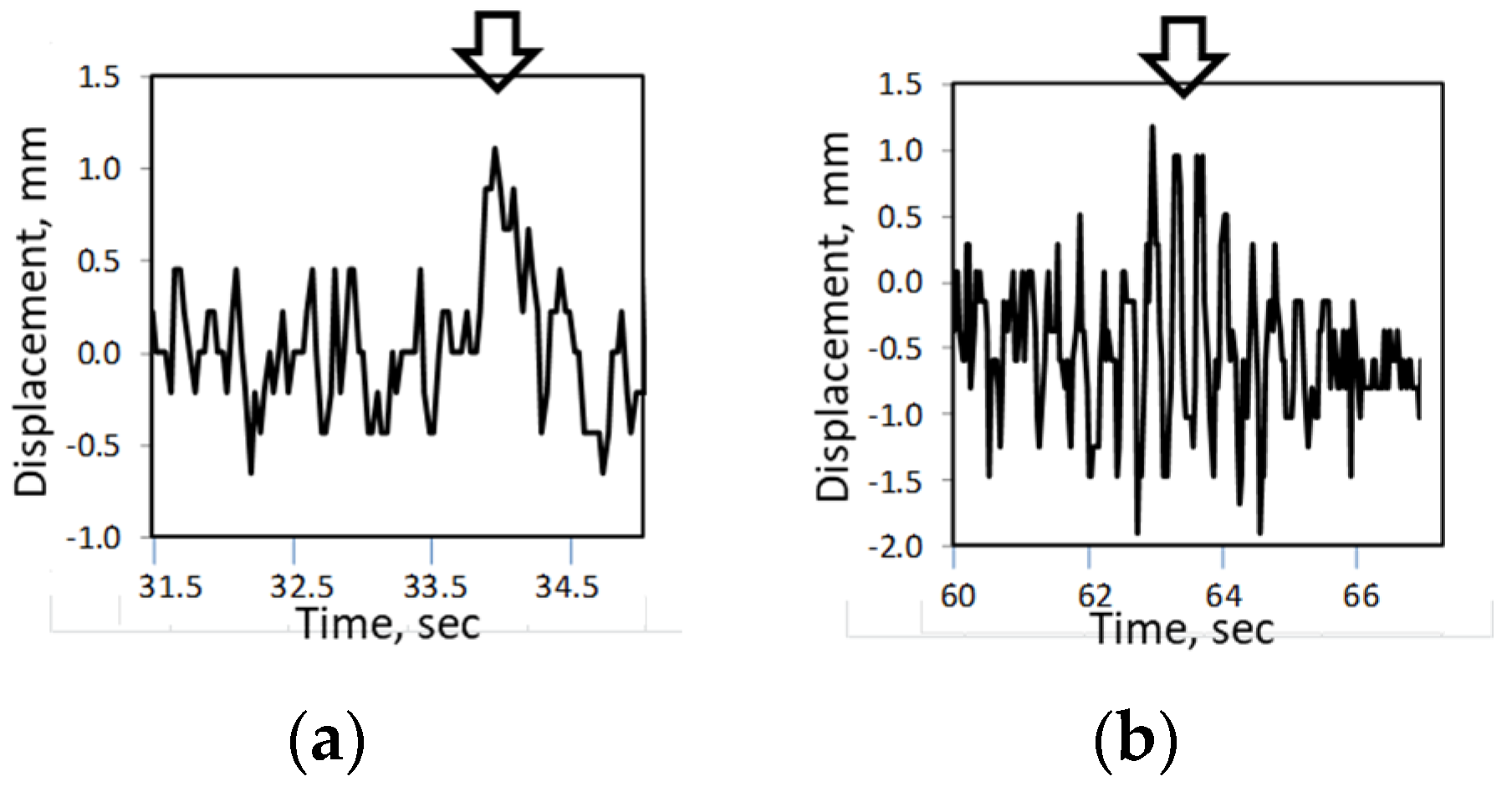
Figure 29.
Layout of simultaneous horizontal and vertical measurements. The direction of measured vibration is indicated on each grid by a thick double-headed arrow.
Figure 29.
Layout of simultaneous horizontal and vertical measurements. The direction of measured vibration is indicated on each grid by a thick double-headed arrow.
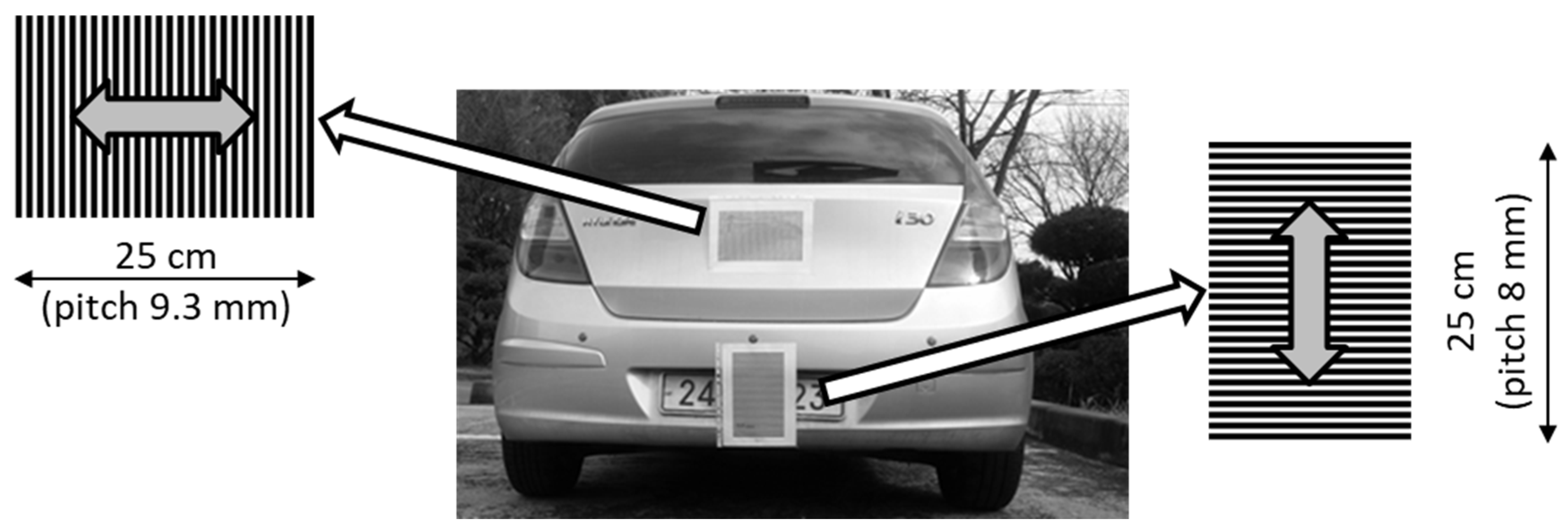
Figure 30.
Simultaneous bidirectional measurements in the car: (a) horizontal component, (b) vertical component.
Figure 30.
Simultaneous bidirectional measurements in the car: (a) horizontal component, (b) vertical component.
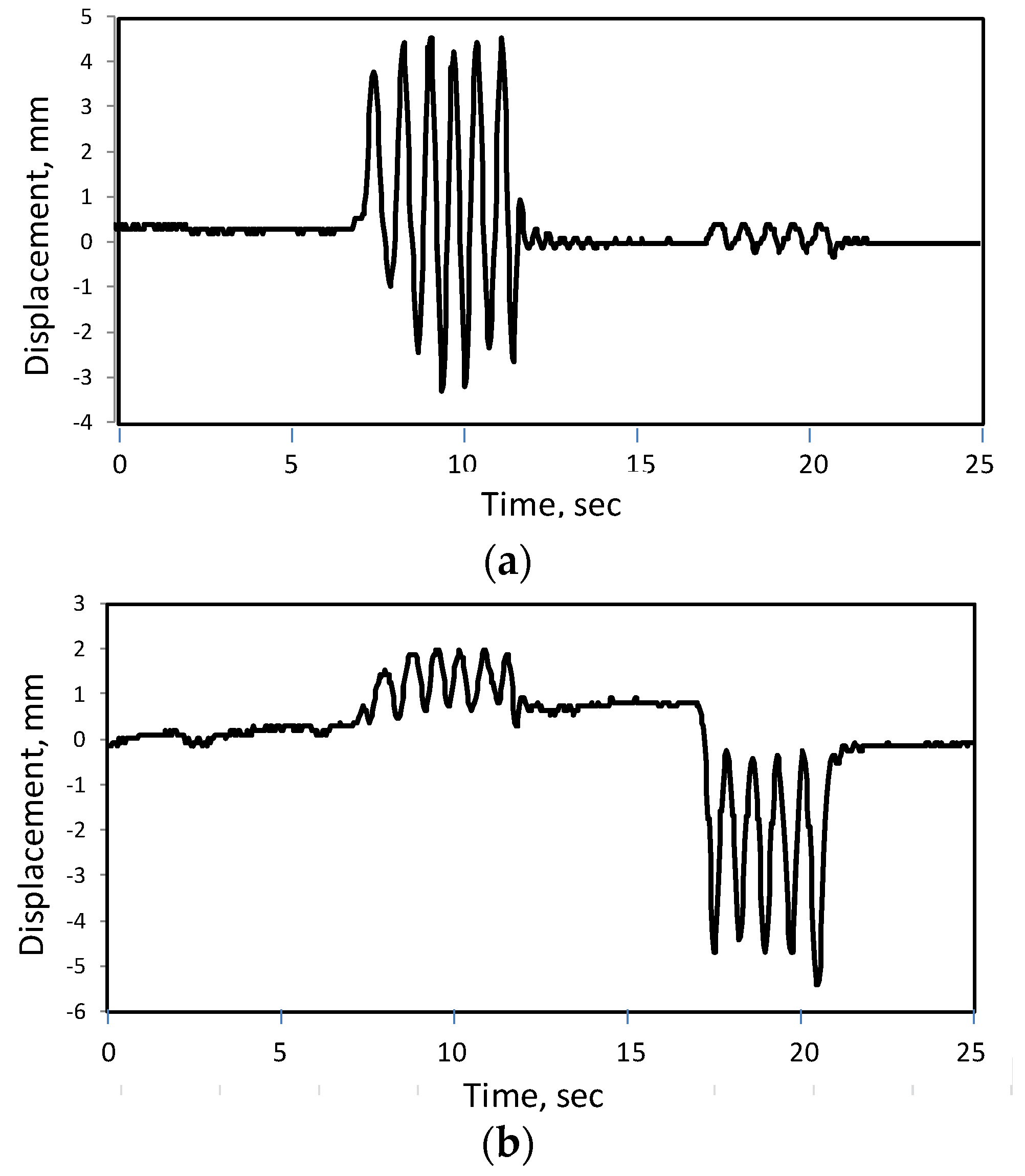
Figure 31.
Scheme and photograph of plastic model (truss railway bridge). Separable plates are numbered.
Figure 31.
Scheme and photograph of plastic model (truss railway bridge). Separable plates are numbered.
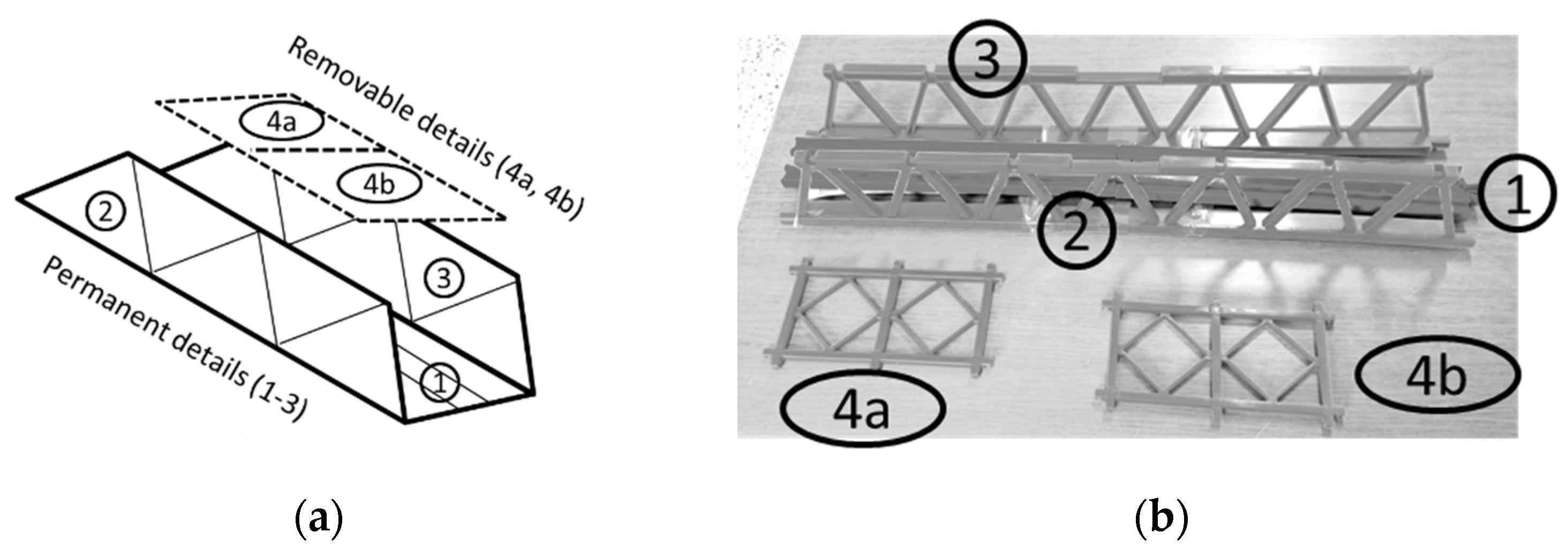
Figure 32.
Layout of experiment with the model of a railway bridge.
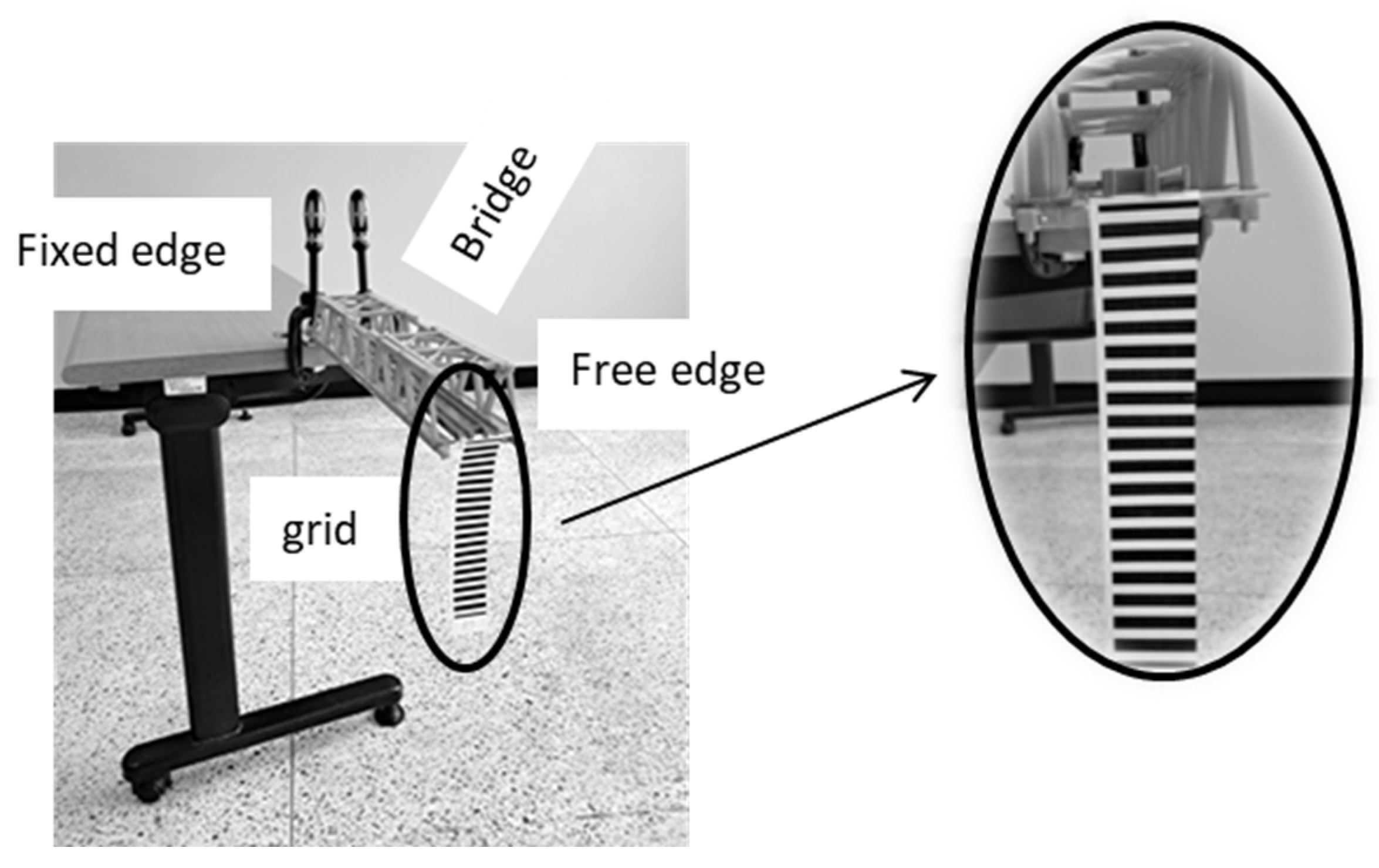
Figure 33.
Measured displacement and amplitude after impact.
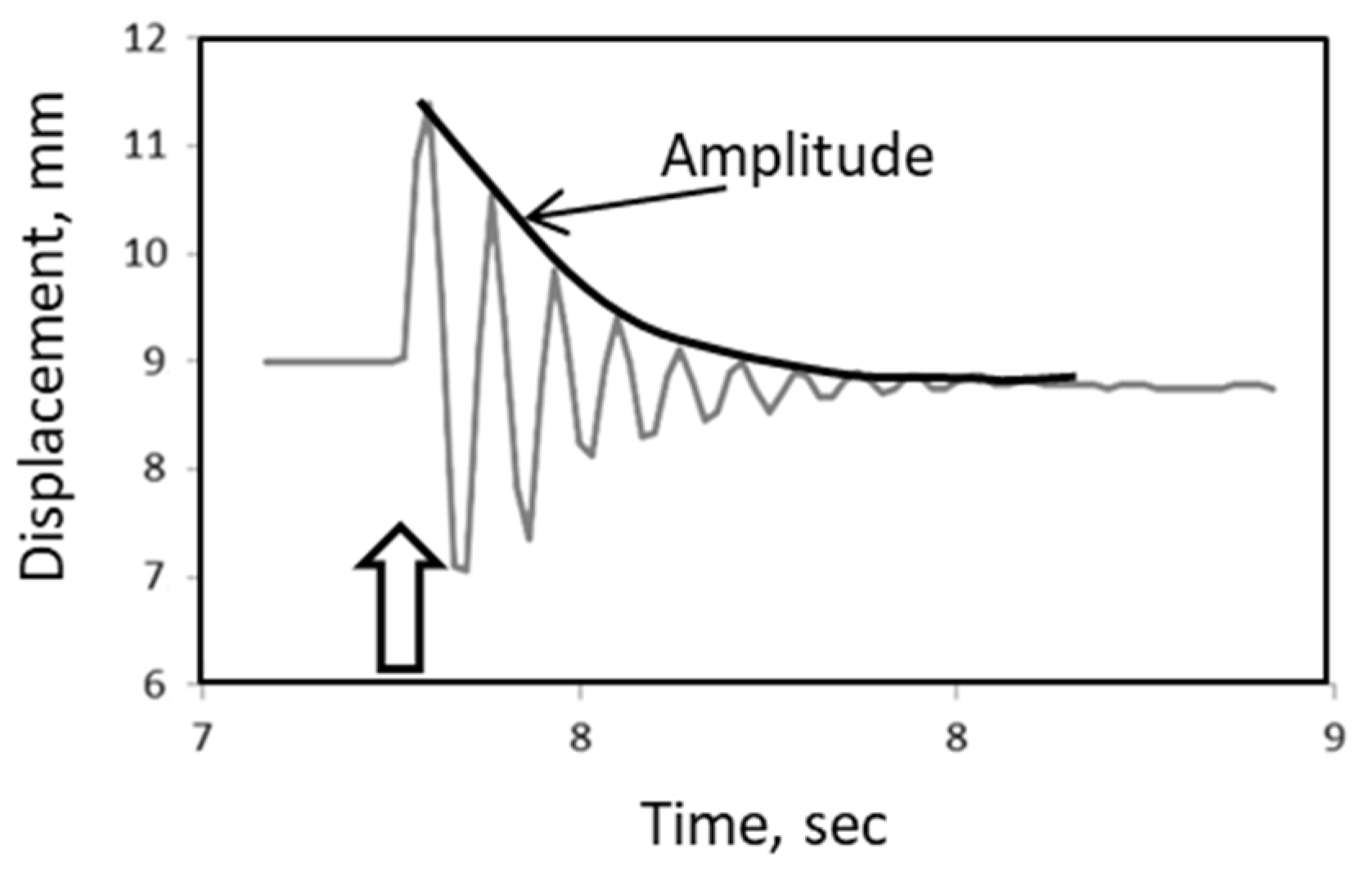
Figure 34.
Measured characteristics of vibration in parameter space.
Disclaimer/Publisher’s Note: The statements, opinions and data contained in all publications are solely those of the individual author(s) and contributor(s) and not of MDPI and/or the editor(s). MDPI and/or the editor(s) disclaim responsibility for any injury to people or property resulting from any ideas, methods, instructions or products referred to in the content. |
© 2025 by the authors. Licensee MDPI, Basel, Switzerland. This article is an open access article distributed under the terms and conditions of the Creative Commons Attribution (CC BY) license (https://creativecommons.org/licenses/by/4.0/).
Copyright: This open access article is published under a Creative Commons CC BY 4.0 license, which permit the free download, distribution, and reuse, provided that the author and preprint are cited in any reuse.


