
Submitted:
26 June 2025
Posted:
27 June 2025
You are already at the latest version
Abstract
This investigation developed and validated a comprehensive computational framework for solving convection-diffusion-reaction (CDR) equations under convection-dominated conditions through the implementation of Algebraic Sub-grid Scale (ASGS) stabilization coupled with high-order finite elements. The research addressed the fundamental challenge of spurious oscillations that emerge in standard Galerkin formulations when convection significantly exceeds diffusion, a prevalent issue in transport phenomena modeling. A novel Python-based educational software platform, designated CDR-Solv, was engineered to demonstrate the effectiveness of ASGS stabilization across polynomial degrees ranging from linear to cubic elements. Numerical experiments conducted with low diffusion coefficients demonstrated that the ASGS method successfully eliminated numerical instabilities while maintaining solution accuracy across diverse source term configurations. The stabilization parameter τK proved instrumental in achieving computational stability without compromising mathematical rigor. Comparative analysis revealed that higher-order elements consistently outperformed linear approximations in capturing boundary layer phenomena and sharp gradient regions. The primary contribution of this work lies in the development of an open-source educational platform that democratizes access to advanced stabilization techniques while providing transparency in algorithmic implementation. The CDR-Solv framework enables researchers and educators to systematically explore the relationship between polynomial degree selection and solution quality in convection-dominated regimes.
Keywords:
convection-diffusion-reaction
; stabilized finite element methods
; high order
; numerical integration
; Python
1. Introduction
The convection-diffusion-reaction equation, a partial differential equation, describes the transport of substances, energy, and other physical quantities within systems. This equation is widely used in many scientific and engineering disciplines [1,2,3].
1.1. Equation
The general form of the stationary scalar convection-diffusion-reaction equation is expressed in equation (1):
where, represents the concentration, which is an unknown scalar variable, is the velocity vector associated with convection, is the diffusion coefficient, is the reaction coefficient, and is the known source term.
1.2. Concepts
Diffusion is the dispersion of particles or energy from areas of high concentration to areas of low concentration due to random molecular motion. In an equation, diffusion is usually represented by a term involving a diffusion coefficient and the second spatial derivative of the quantity being transported.
Convection involves the transport of a substance or energy due to the motion of a fluid’s mass. The convection term in the equation generally includes fluid velocity and the spatial derivative of the transported quantity. The reaction term accounts for the generation or consumption of the transported quantity due to chemical or biological reactions. The reaction term includes a coefficient and the quantity being transported.
1.3. Solution Methods
The convection-diffusion-reaction equation can be solved using analytical or numeri-cal methods. Analytical solutions are exact but generally limited to simplified cases with specific boundary conditions.
Numerical methods approximate solutions by discretizing equations and domains. These methods are necessary when analytical solutions are unavailable or when the geo-metry or problem is too complex for exact solutions [4].
Some examples of numerical methods are:
1.3. Galerkin’s Method
The Galerkin method is a widely used numerical technique for approximating solutions to the convection-diffusion-reaction equation. It belongs to the family of weighted residual methods and forms the basis of the finite element method (FEM). The key idea behind the Galerkin method (Hernández Marulanda & Gaviria Posada, 2020) is to find an approximate solution within a finite-dimensional space by minimizing error when the approximate solution is inserted into the original equation [10].
1.3.1. Variational Formulation
The Galerkin method begins by converting the original differential equation into its variational form. This involves multiplying the equation by a test function and integrating by parts over the domain. This reduces the original problem to first-order derivatives, which is a key feature for using relatively simple approximation spaces.
1.3.2. Approach Space
The Galerkin method approximates solutions using subspaces of finite-dimensional functions [8,11]. This subspace is typically constructed using polynomial-shaped functions. The choice of the approximation space is crucial. Finite element spaces, which are defined by a domain mesh and a set of shape functions on each mesh element, are often used [12,13].
1.3.3. Galerkin Discretization
The variational form of the equation is solved using functions of a finite-dimensional space [11]. This expression is a linear combination of shape functions within the chosen finite-dimensional space.
This method requires the variational form of the equation to be satisfied for all test functions within the same space. This results in a system with an equal number of linearly independent equations and unknowns. These unknowns correspond to the nodal values of the variable [12].
1.3.4. Error Analysis
Error analysis is important for determining the accuracy of an approximation. Optimal error estimates can be derived for certain Galerkin methods when assumptions are made about the regularity of the exact solution. Factors such as the choice of numerical scheme or irregularities in the mesh can affect the rate of convergence [14,15].
1.3.5. Instability
The Galerkin method can become unstable in problems with dominant convection (), which can lead to spurious oscillations in the numerical solution.
Several stabilization techniques have been developed to overcome these problems. These techniques modify the Galerkin method to reduce oscillations, thereby improving the stability and accuracy of the numerical solution. Some of these techniques are:
1.4. Related Works
The numerical solution of convection-diffusion-reaction (CDR) equations has evolved through diverse methodological approaches, each addressing specific computational challenges while contributing unique innovations to the field. Traditional finite element methodologies have been extensively refined to overcome inherent limitations in convection-dominated problems. Nadukandi et al. pioneered the development of high-resolution Petrov-Galerkin (HRPG) finite element methods for one-dimensional CDR problems, systematically addressing spurious oscillations through novel stabilization parameters derived from discrete upwinding operations and mass-lumping techniques [20]. Their approach incorporated both streamline upwinding and discontinuity-capturing operators within a nonlinear Petrov-Galerkin formulation using linear elements, demonstrating superior performance compared to established SUPG, CAU, and modified CAU methods by achieving second-order accuracy in smooth regimes while maintaining excellent shock-capturing capabilities. Building upon this foundation, [21] extended the HRPG methodology to multidimensional scenarios, employing lowest-order block finite elements combined with objective characteristic tensors to achieve frame-independent stabilization parameters. Their implementation utilized bilinear block finite elements with temporal discretization through the generalized trapezoidal method, solved via Picard methodology with convergence tolerance of 1e-5, demonstrating superior layer resolution compared to existing stabilized methods while effectively handling exponential and parabolic boundary layers. Lima et al. in 2021 [22] contributed to traditional finite element approaches by implementing the Galerkin Finite Element Method with comprehensive error correlation analysis, utilizing linear shape functions over standardized domains and employing MATLAB for numerical computations and visualization. Their methodology addressed nonlinear parabolic partial differential equations without truncating nonlinear terms, achieving exceptional convergence properties with absolute errors ranging from to depending on mesh refinement, while demonstrating versatility across diverse engineering applications including neutron diffusion and pollutant transport modeling.
Innovative hybrid and meshless approaches have emerged to address computational limitations of traditional discretization methods. In 2012 Shirzadi et al. [23] developed a superior numerical framework combining Meshless Local Petrov-Galerkin (MLPG) formulation with specialized finite difference approximations for Caputo fractional derivatives, creating a hybrid weak-form solution strategy for two-dimensional fractional-time CDR equations. Their implementation featured circular subdomains with sophisticated adaptive stepping algorithms and eight-point Legendre-Gauss quadrature formulations, demonstrating capability to handle convection coefficients ranging from to , substantially exceeding limitations of strong-form methodologies. Liu et al. in 2021 [24] advanced meshless methodologies by developing localized method of fundamental solutions (LMFS) for transient CDR equations, combining Crank-Nicolson time-stepping with pseudo-spectral Chebyshev collocation schemes in their CN-CCS-LMFS approach. Their MATLAB implementation utilized ‘gmres’ and ‘pinv’ functions with specific tolerance settings, transforming dense matrix structures into sparse, banded systems through domain decomposition techniques, enabling large-scale dynamic simulations previously computationally prohibitive while maintaining accuracy comparable to traditional methods. In 2011 Theeraek et al. [25] contributed an innovative adaptive finite volume element method that combined cell-centered finite volume discretization with finite element concepts, implementing second-order accuracy through Taylor series expansion along local characteristic lines. Their approach integrated adaptive meshing utilizing advancing front methodology with weighted residuals methods from finite element theory, successfully eliminating spurious oscillations while optimizing computational efficiency through dynamic element size adjustment based on principal stress concepts from solid mechanics theory.
Specialized high-order and spectral methodologies have been developed to achieve superior accuracy with reduced computational requirements. In 2022 Mkhatshwa and Khumalo [26] introduced a novel trivariate spectral collocation approach (TSQLM) for three-dimensional elliptic partial differential equations, employing quasilinearization methods combined with triple Lagrange interpolating polynomials established via Chebyshev-Gauss-Lobatto nodes. Their MATLAB 2015a implementation utilized specialized functions including kron() for Kronecker products and superkron() for multi-matrix operations, achieving exceptional accuracy with absolute errors approaching 10−17 using minimal grid sizes of 15×15×15, significantly outperforming existing methods that required thousands of discretization points for equivalent precision. Wei et al. in 2022 [27] developed innovative high-order compact (HOC) finite difference methods utilizing fourth-order Padé approximation schemes combined with Taylor series expansion and truncation error remainder correction, achieving fourth-order spatial accuracy and second-order temporal accuracy. Their methodology employed minimal computational stencils of five points for 2D and seven points for 3D problems compared to traditional approaches requiring 9-27 point stencils, implementing successive over-relaxation iterative methods with PHOEBESolver software for validation, demonstrating unconditional stability for variable coefficient problems where existing HOC methods typically face stability limitations. In 2021 Ullmann et al. [28] contributed specialized reduced basis methodologies by implementing Stochastic Galerkin Reduced Basis (SGRB) and Monte Carlo Reduced Basis (MCRB) approaches for parameter-dependent statistics estimation. Their implementation employed finite element discretization using continuous piecewise linear elements with 225 to 961 degrees of freedom, utilizing polynomial chaos expansions with Legendre polynomials and proper orthogonal decomposition for snapshot-based reduced space generation, demonstrating that approximately 16 reduced basis functions sufficed for accurate statistical estimates while providing computational speedup proportional to Monte Carlo sample sizes.
Surface-based and advanced flux correction methodologies have addressed specialized geometric and physical constraints. Xiao et al. in 2019 [29] developed adaptive finite element methodology specifically for CDR equations on curved surfaces, combining Surface Finite Element Method (SFEM) with Streamline Diffusion Method (SDM) for stabilization and Zienkiewicz-Zhu gradient recovery-based error estimation for adaptive mesh refinement. Their implementation employed piecewise linear finite elements on curved triangular meshes with local Delaunay algorithm refinement strategies, achieving convergence rates between 1.7-5.0 while successfully capturing complex solution behaviors including spiral-type curves and internal layers on spherical and toroidal surfaces. It worths to mention the prior work of Zalesak [30], that addressed critical limitations of flux-corrected transport algorithms by developing fully multidimensional flux limiting techniques implemented through sophisticated finite difference approaches in conservation form. Their vectorized Fortran implementation on Texas Instruments ASC computer employed leapfrog-trapezoidal transport algorithms with varying spatial accuracy orders from second to eighth order, combining low-order monotonic schemes with high-order schemes through novel six-step procedures that simultaneously considered antidiffusive fluxes in all coordinate directions, effectively eliminating “clipping” phenomena while maintaining sharp discontinuity resolution over 2-4 grid points without numerical oscillations.
Analytical and specialized mathematical approaches have provided alternatives to purely numerical methodologies. In 2022 Parhizi et al. [31] diverged from traditional numerical approaches by developing comprehensive Green’s function-based methodology for arbitrary source terms in CDR equations, employing mathematical transformation approaches through variable substitution and separation of variables techniques to derive eigenvalue-based solutions. Their purely analytical framework eliminated computational instabilities commonly encountered in finite element and finite difference methods, requiring only 7-25 eigenvalues for convergence across different Péclet numbers with computation times of 0.4-3.3 seconds compared to 4.1 seconds for conventional numerical methods, while providing superior accuracy and computational speed for complex transport phenomena including drug delivery systems and contaminant dispersion applications. These diverse methodological approaches collectively demonstrate the evolution of numerical techniques for CDR equations, from traditional finite element formulations through innovative meshless and hybrid methods to specialized high-order schemes and analytical frameworks, each contributing unique computational advantages while addressing specific challenges in accuracy, stability, and computational efficiency across various physical applications and geometric constraints.
Complementarly to these previous studies, this work focuses on the Galerkin method and thoroughly explores the Algebraic Subgrid Scale (ASGS) stabilization method, employing third-order finite elements to improve numerical solution accuracy. Additionally, computational didactic software was developed in Python and made freely available on GitHub.
2. Materials and Methods
2.1. Mathematical Models
The stationary scalar convection-diffusion-reaction equation (2) was used, where was searched for using numerical methods.
where is the unknown scalar variable in , is the diffusion coefficient, is the convective velocity field for incompressible flow, is the reaction coefficient, and is the known source term. The Dirichlet boundary conditions are known along the boundary .
Integrating equation (2) by parts yields the continuous variational form of the problem, which is to find such that:
by partitioning the domain , we obtain the discretized integral equation that allows us to find . Where, is the number of elements in the partition, and is the domain of the element:
to numerically calculate the integrals of equation (4), we approximate the variable in the domain with by interpolating with functions called shape functions, given by:
where is the number of nodes in the finite element and is the nodal value of the function at the node , is the polynomial form of the function such that it equals one at node and zero at the other nodes in the finite element.
By replacing equation (5) and using the Galerkin method for , we obtain the standard Galerkin formulation. This formulation can be used to solve the stationary scalar convection-diffusion-reaction equation numerically using a computational algorithm developed in Python:
2.2. Shape Functions
Shape functions enable the numerical calculation of the convection-diffusion-reaction equation. In the present case, the functions must be of class , i.e., they must be continuous. Continuity depends on how the functions are connected element by element, rather than how they are interpolated within them. Lagrange class elements, the most common in the finite element method, belong to class , while Hermite class elements belong to class .
The model used contains second derivatives in the convection-diffusion-reaction equation. When weakened with the variational form, the largest derivatives are of first order. Therefore, class shape functions are required to satisfy continuity between elements, and at a minimum, linear shape functions are required to obtain mesh convergence. Test functions must have the same continuity conditions as shape functions to approximate the unknown function .
2.3. Regular Mesh
The equation is solved for a rectangular area with sides and . Given the number of elements into which each side of the rectangle is divided and the degree of the polynomial of the shape functions, a grid is generated in which each intersection corresponds to a node. The nodes are numbered globally from bottom to top and from left to right, including the edges. The total number of nodes, including the edges, is , and the total number of nodes inside the mesh, excluding the edges, is . This corres-ponds to the number of unknowns because the values of the function at the edges are known, as the Dirichlet conditions are prescribed at the boundary. The total number of triangular elements is .
Figure 1a presents an example of the global node numbering (points with numbers) and triangular element numbering (enclosed numbers) for a single segment on each side of the rectangle and for three polynomial degrees of linear (), quadratic (), and cubic () shape functions.
Figure 1b shows the local numbering of nodes in a triangular element for the three polynomial degrees. Local numbering allows for consistent referencing of nodes forming a triangular element, which is required in the connectivity matrix.
2.4. Connectivity Matrix
The connectivity matrix containing rows is generated based on the number of elements into which each side of the rectangle is divided and the degree of the polynomial of the shape functions. Each row of the connectivity matrix corresponds to a triangular element. For each triangular element, a list of node numbers is placed based on the global node numbering (see Figure 1a). This list must follow the sequence given by the local node numbering (see Figure 1b).
2.5. Elementary Matrix and Force Vector
The elementary matrix and force vector are generated for each triangular element, considering the parameters defined in the stationary scalar convection-diffusion-reaction equation statement.
In the standard Galerkin formulation, the element matrix of equation (7) and the force vector of equation (8) are unstable in the case of dominant convection:
applying ASGS stabilization yields the stable element matrix with equation (9) and the stable force vector with equation (10):
in equations (9) and (10), the stabilization parameter, , is given by Equation (11):
2.6. User Interface
A Python program was developed, which allows the user to configure constants, source terms, and Dirichlet boundary conditions via a user interface. The program then uses Python functions to obtain the solution, which is displayed as three- and two-dimensional plots.
The functions used are:
- main_cdr.py: This is the main file that contains initialization, the user interface, and all the used functions;
- get_config: This function retrieves all data entered in the user interface and verifies it;
- nodes: This function creates the regular mesh. The first column is the X coordinate, the second column is the Y coordinate, and each row represents a different node. The order of the nodes in this matrix determines the overall node numbering;
- tc3: This function generates the connectivity matrix. As shown in Figure 2, each row represents a triangular element and its component nodes;
- cccnpg: A function that transforms Cartesian coordinates to natural coordinates at a Gauss point;
- kefe2DT: A function that obtains the elemental matrix and force vector, corrected according to ASGS stabilization;
- ffT: A function that generates shape functions and their derivatives at a Gauss point for a given polynomial degree;
- vffydp2DT: Calculates the values of the shape functions and their partial derivatives at all Gauss points for triangular elements and all polynomial degrees;
- gauss2DT: Function to obtain matrices with Gauss weights and points;
- es2: Assembles and solves the system of equations under the entered parameters.
3. Results
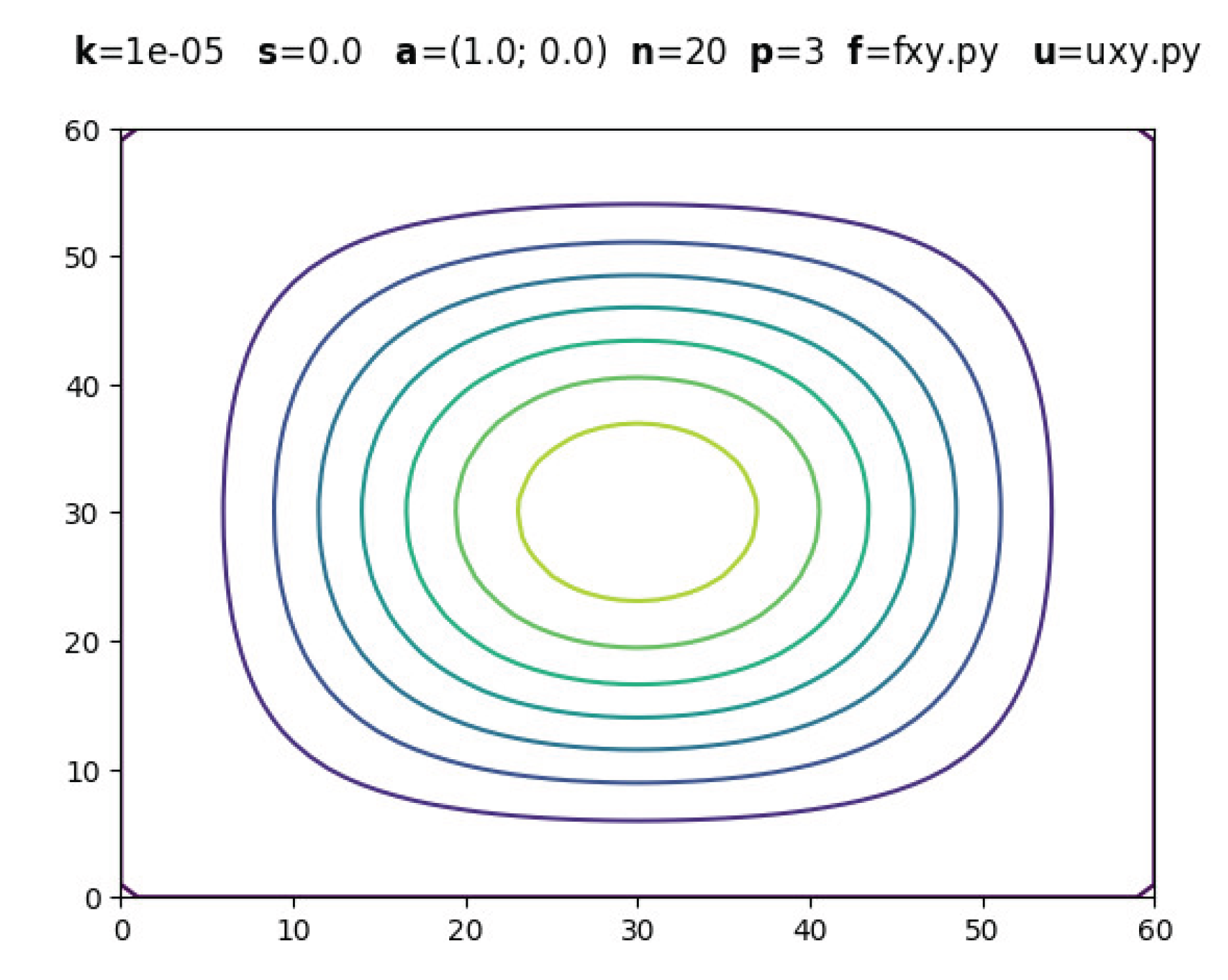
The following figures are screenshots of those generated with boundary layers. In all examples, is used to ensure dominant convection while maintaining , .
3.1. Evolution with Polynomial Degree
3.1. Other Functions for Source Term
4. Discussion
The present investigation successfully demonstrated the effectiveness of combining the Algebraic Sub-grid Scale (ASGS) stabilization method with high-order finite elements for solving convection-diffusion-reaction equations in convection-dominated regimes. The computational framework developed in Python, designated as CDR-Solv, provided robust numerical solutions across multiple polynomial degrees and source term configurations, establishing a significant contribution to the field of computational fluid dyna-mics and transport phenomena modeling.
The numerical experiments conducted with various polynomial degrees () consistently demonstrated the superior performance of higher-order elements in captu-ring solution features, particularly in boundary layer regions where convection dominates diffusion (). The implementation achieved stable solutions across all tested configurations, effectively eliminating the spurious oscillations that typically plague standard Galerkin formulations in convection-dominated problems. The stabilization parameter proved crucial in maintaining numerical stability while preserving solution accuracy, demonstrating the theoretical soundness of the ASGS approach.
When compared to previous investigations detailed in the related works section, the current study distinguished itself through several key aspects. Unlike the meshless approaches of [23,24], which focused on fractional-time and localized fundamental solutions respectively, the present work employed a stabilized finite element framework that maintains the mathematical rigor of variational formulations while providing computational efficiency through structured mesh implementations. The ASGS method implemented herein offered distinct advantages over the High-Resolution Petrov-Galerkin (HRPG) approaches of [20,21], particularly in terms of implementation simplicity and computational cost, as ASGS does not require complex stabilization parameter calibration for different physical regimes.
The spectral accuracy achievements of [26] with their trivariate spectral collocation approach (TSQLM) represented a different paradigm, targeting exceptional precision through minimal grid points but requiring specialized mathematical formulations. In contrast, the CDR-Solv framework prioritized accessibility and educational value through its open-source Python implementation, making advanced stabilization techniques available to a broader scientific community. The present study’s approach proved more versatile than the analytical Green’s function methodology of [31], which, while computationally efficient for specific source terms, lacked the flexibility to handle arbitrary geometric configurations and complex boundary conditions.

Table 1.
Advantages and limitations for related works.
| Name | Technique | Advantages | Limitations |
|---|---|---|---|
| CDR-Solv (Present Study) | ASGS stabilization with Python implementation | Open-source accessibility, educational value, high-order finite elements up to p=3, robust stabilization, user-friendly interface | Limited to structured meshes, requires Python environment |
| Nadukandi et al. (2010) | High-Resolution Petrov-Galerkin (HRPG) with linear elements | Superior shock-capturing, second-order accuracy in smooth regimes | Complex parameter calibration, limited to 1D problems, requires specialized implementation |
| Liu et al. (2021) | Localized Method of Fundamental Solutions (LMFS) with MATLAB | Meshless approach, sparse matrix structure, large-scale capability | Requires MATLAB license, complex mathematical formulation, limited geometric flexibility |
| Mkhatshwa & Khumalo (2022) | Trivariate Spectral Collocation (TSQLM) with MATLAB | Exceptional accuracy (10−17), minimal grid points, spectral convergence | MATLAB dependency, limited to elliptic problems, requires specialized mathematical expertise |
| Parhizi et al. (2022) | Green’s Function analytical approach | Pure analytical framework, superior computational speed, exact solutions | Limited to specific source terms, complex mathematical derivations, restricted geometric applications |
The ASGS stabilization method represented a fundamental advancement over traditional approaches by providing consistent stabilization across different convection regimes without requiring problem-specific parameter tuning. This distinguished the present work from the finite volume element method of [25], which, while effective for adaptive meshing, required complex stability analysis and CFL-like restrictions. The ASGS formulation inherently addressed the Gibbs phenomenon and spurious oscillations through its multiscale variational approach, offering theoretical advantages over ad-hoc stabilization techniques.
The educational and accessibility contributions of the CDR-Solv framework cannot be understated in the context of scientific software development. Unlike proprietary solutions or specialized academic codes, the open-source Python implementation provided several critical advantages: (1) complete transparency in algorithmic implementation, enabling reproducible research and educational applications; (2) cross-platform compatibility without licensing restrictions; (3) integration with the extensive Python scientific computing ecosystem; and (4) accessibility to researchers and students in developing countries where commercial software licenses may be prohibitive. This philosophical approach aligned with the growing movement toward open science and reproducible computational research. The didactic value of the CDR-Solv implementation extended beyond mere algorithmic availability. The modular structure of the code, with clearly defined functions for mesh generation (nodes, tc3), element matrix assembly (kefe2DT), and shape function evaluation (ffT, vffydp2DT), provided an educational framework for understanding finite element implementation details. This contrasted sharply with black-box commercial solutions or highly optimized research codes that obscure fundamental mathematical concepts.
The significance of employing ASGS stabilization extended beyond numerical considerations to theoretical implications for multiscale phenomena modeling. The method’s ability to capture subgrid-scale effects without explicit mesh refinement provided computational efficiency advantages, particularly relevant for problems with boundary layers or sharp gradients. This theoretical foundation distinguished the approach from purely numerical stabilization techniques that lack rigorous mathematical justification.
Future research directions for this work include extension to three-dimensional geometries, implementation of adaptive mesh refinement capabilities, and integration with high-performance computing frameworks for large-scale applications, which we believe are crucial as mentioned by [29] but are out of the scope of this study. The open-source nature of the CDR-Solv platform provides a foundation for collaborative development and community-driven enhancements, potentially leading to more sophisticated and specialized implementations for specific application domains.
5. Conclusions
This investigation successfully established the efficacy of implementing Algebraic Sub-grid Scale (ASGS) stabilization techniques in conjunction with high-order finite element methodologies for addressing convection-diffusion-reaction equations under convection-dominated flow regimes. The research demonstrated that the developed computational framework, designated CDR-Solv, achieved remarkable numerical stability and accuracy across polynomial degrees ranging from linear to cubic formulations (), effectively mitigating the spurious oscillations that traditionally compromise standard Galerkin approaches in transport-dominated scenarios. The stabilization parameter formulation proved instrumental in maintaining solution convergence while preserving computational efficiency, thereby validating the theoretical foundations of the multiscale variational approach inherent to ASGS methodology. Extensive numerical experimentation across diverse source term configurations, including constant, linear, polynomial, and analytical benchmark functions, consistently yielded stable and physically meaningful solutions, particularly in boundary layer regions where conventional finite element methods typically exhibit instability.
The implementation of third-order finite elements within the ASGS framework represented a significant advancement in achieving superior solution accuracy without compromising computational tractability, distinguishing this work from existing methodologies that often require complex parameter calibration or specialized mathematical formulations. A paramount contribution of this research resided in the development and open-source distribution of educational software that democratizes access to advanced stabilization techniques, fostering reproducible computational research and providing valuable pedagogical resources for the scientific community.
The Python-based implementation offered unprecedented transparency in algorithmic development, enabling researchers and students worldwide to examine, modify, and extend the computational framework without proprietary restrictions or licensing barriers. This philosophical commitment to open science facilitated knowledge transfer and collaborative enhancement of numerical methods for transport phenomena modeling. The modular software architecture, featuring clearly delineated functions for mesh generation, connectivity matrix assembly, and stabilized element formulation, served as an exemplary educational platform for understanding finite element implementation fundamentals. Furthermore, the cross-platform compatibility and integration with the broader Python scientific computing ecosystem positioned CDR-Solv as a versatile tool for diverse engineering applications spanning environmental modeling, chemical reactor design, and heat transfer analysis. The comparative analysis with existing methodologies revealed distinct advantages of the ASGS approach over alternative stabilization techniques, particularly regarding implementation simplicity, computational cost-effectiveness, and robustness across varying physical parameter ranges. These findings collectively established ASGS stabilization as a superior methodology for convection-dominated transport problems while simultaneously contributing a valuable computational resource that advances both theoretical understanding and practical application of stabilized finite element methods in the broader scientific community.
Author Contributions
Investigation, A.P.V.-C., I.P.S.-P., and G.F.G.-V.; conceptualization, A.P.V.-C., I.P.S.-P., and G.F.G.-V.; Methodology, E.P.H.-G., A.P.V.-C., I.P.S.-P., and G.F.G.-V.; supervision, E.P.H.-G., A.P.V.-C., I.P.S.-P., and G.F.G.-V.; writing—original draft preparation, E.P.H.-G., A.P.V.-C., I.P.S.-P., and G.F.G.-V.; writing—review and editing, E.P.H.-G., A.P.V.-C., I.P.S.-P., and G.F.G.-V.; funding acquisition, A.P.V.-C., and I.P.S.-P. All authors have read and agreed to the published version of the manuscript.
Funding
This work was supported by the National Polytechnic School - EPN of Ecuador (www.epn.edu.ec accessed on 28 May 2025).
Data Availability Statement
The Python program is available for download and editing at the following link: https://github.com/angel-villota/CDR-Solv/blob/main/PythonCode.zip. A pre-assembled executable for Windows is available at the following links: https://github.com/angel-villota/CDR-Solv/blob/main/executable.zip.001; https://github.com/angel-villota/CDR-Solv/blob/main/executable.zip.002.
Acknowledgments
We acknowledge the National Polytechnic School - EPN of Ecuador for their support in carrying out this research.
Conflicts of Interest
The authors declare no conflicts of interest.
References
- R. Cachay Torres, “Influencia del término difusivo en el modelamiento de transporte de masa usando la ecuación de convección difusión no lineal,” Universidad Nacional de Trujillo, 2024. [Online]. Available: https://dspace.unitru.edu.pe/items/756435db-e611-4478-8241-7f1be2b71638.
- C. P. Castro Torres, “Evaluación de la concentración de material radiactivo disperso en la atmósfera a través de la ecuación de difusión: Solución de la ecuación de advección para la liberación instantánea de contaminantes,” ESCUELA POLITÉCNICA NACIONAL, 2023. [Online]. Available: https://bibdigital.epn.edu.ec/handle/15000/24851.
- C. H. Galeano, J. M. Mantilla, and D. A. Garzón-Alvarado, “Experimentos numéricos sobre ecuaciones de reacción convección difusión con divergencia nula del campo de velocidad,” Rev. Int. métodos numéricos para cálculo y diseño en Ing., vol. 26, no. 2, pp. 69–81, 2010, [Online]. Available: https://core.ac.uk/download/pdf/41822303.pdf.
- J. A. M. López, “Análisis numérico de un método de Galerkin para un problema evolutivo no lineal,” Universidad de Córdoba, 2024. [Online]. Available: https://repositorio.unicordoba.edu.co/entities/publication/7f44654d-3d7b-4993-8ea8-020412477bd2.
- A. F. Hernández Marulanda and L. J. Gaviria Posada, “Solución de la ecuación de convección difusión mediante las funciones de base radial multicuádricas,” Ing. USBMed, vol. 11, no. 2, pp. 48–53, Oct. 2020. [CrossRef]
- F. C. Osorio Guzman, P. A. Amador Rodriguez, and C. A. Bedoya Parra, “Solución Numérica de una ecuación de convección-difusión no local fraccionaria,” Entre Cienc. e Ing., vol. 18, no. 35, pp. 25–31, Jun. 2024. [CrossRef]
- Peinado Asensi, “Resolución de ecuaciones de convección-difusión en 2D usando el método de las diferencias finitas compactas,” Universitat Politècnica de València, 2019. [Online]. Available: https://riunet.upv.es/handle/10251/129534.
- T. Coronado González, “Adaptación de mallados de elementos finitos conformes utilizando elementos de tipo hexaedro,” Universidad Politécnica de Madrid, 2021. [Online]. Available: https://oa.upm.es/67850/.
- C. A. Torres Rodríguez, “Desarrollo de código bidimensional transitorio para el estudio de la transferencia de calor en flujo laminar e incompresible aplicado a convección natural con alta variación de relaciones de aspecto,” [sn], 2022. [Online]. Available: https://repositorio.unicamp.br/acervo/detalhe/1242115.
- D. Broersen and R. P. Stevenson, “A Petrov-Galerkin discretization with optimal test space of a mild-weak formulation of convection-diffusion equations in mixed form,” IMA J. Numer. Anal., vol. 35, no. 1, pp. 39–73, Jan. 2015. [CrossRef]
- M. Benítez and B. Cockburn, “Post-processing for spatial accuracy-enhancement of pure Lagrange–Galerkin schemes applied to convection-diffusion equations,” IMA J. Numer. Anal., vol. 42, no. 1, pp. 54–77, Jan. 2022. [CrossRef]
- P. Knobloch and L. Tobiska, “On the stability of finite-element discretizations of convection-diffusion-reaction equations,” IMA J. Numer. Anal., vol. 31, no. 1, pp. 147–164, Jan. 2011. [CrossRef]
- W. Morton, “The convection-diffusion Petrov-Galerkin story,” IMA J. Numer. Anal., vol. 30, no. 1, pp. 231–240, Jan. 2010. [CrossRef]
- Y. Chen and B. Cockburn, “Analysis of variable-degree HDG methods for convection-diffusion equations. Part I: general nonconforming meshes,” IMA J. Numer. Anal., vol. 32, no. 4, pp. 1267–1293, Oct. 2012. [CrossRef]
- V. Dolejsi, M. Feistauer, V. Kucera, and V. Sobotikova, “An optimal L (L2)-error estimate for the discontinuous Galerkin approximation of a nonlinear non-stationary convection-diffusion problem,” IMA J. Numer. Anal., vol. 28, no. 3, pp. 496–521, Nov. 2007. [CrossRef]
- Chen and H. Bagci, “Steady-State Simulation of Semiconductor Devices Using Discontinuous Galerkin Methods,” IEEE Access, vol. 8, pp. 16203–16215, 2020. [CrossRef]
- B. B. King and D. A. Krueger, “The 1-D convection diffusion equation: Galerkin least squares approximations and feedback control,” in 2004 43rd IEEE Conference on Decision and Control (CDC) (IEEE Cat. No.04CH37601), IEEE, 2004, pp. 1502-1507 Vol.2. [CrossRef]
- H. Gómez, I. Colominas, F. L. Navarrina Martínez, and M. Casteleiro Maldonado, “Un nuevo enfoque para el tratamiento de los términos difusivos en la ecuación de convección-difusión en el método de Galerkin discontinuo,” Rev. Int. métodos numéricos para cálculo y diseño en Ing., vol. 23, no. 4, pp. 343–362, 2007, [Online]. Available: https://engineering.purdue.edu/gomez/assets/pdf/art03.pdf.
- H. Chen, J. Li, and W. Qiu, “Robust a posteriori error estimates for HDG method for convection–diffusion equations,” IMA J. Numer. Anal., vol. 36, no. 1, p. drv009, Mar. 2015. [CrossRef]
- P. Nadukandi, E. Oñate, and J. Garcia, “A high-resolution Petrov–Galerkin method for the 1D convection–diffusion–reaction problem,” Comput. Methods Appl. Mech. Eng., vol. 199, no. 9–12, pp. 525–546, Jan. 2010. [CrossRef]
- P. Nadukandi, E. Oñate, and J. García, “A high-resolution Petrov–Galerkin method for the convection–diffusion–reaction problem. Part II—A multidimensional extension,” Comput. Methods Appl. Mech. Eng., vol. 213–216, pp. 327–352, Mar. 2012. [CrossRef]
- S. A. Lima, M. Kamrujjaman, and M. S. Islam, “Numerical solution of convection–diffusion–reaction equations by a finite element method with error correlation,” AIP Adv., vol. 11, no. 8, Aug. 2021. [CrossRef]
- A. Shirzadi, L. Ling, and S. Abbasbandy, “Meshless simulations of the two-dimensional fractional-time convection–diffusion–reaction equations,” Eng. Anal. Bound. Elem., vol. 36, no. 11, pp. 1522–1527, Nov. 2012. [CrossRef]
- S. Liu, P.-W. Li, C.-M. Fan, and Y. Gu, “Localized method of fundamental solutions for two- and three-dimensional transient convection-diffusion-reaction equations,” Eng. Anal. Bound. Elem., vol. 124, pp. 237–244, Mar. 2021. [CrossRef]
- P. Theeraek, S. Phongthanapanich, and P. Dechaumphai, “Solving convection-diffusion-reaction equation by adaptive finite volume element method,” Math. Comput. Simul., vol. 82, no. 2, pp. 220–233, Oct. 2011. [CrossRef]
- P. Mkhatshwa and M. Khumalo, “Trivariate Spectral Collocation Approach for the Numerical Solution of Three-Dimensional Elliptic Partial Differential Equations,” Mathematics, vol. 10, no. 13, p. 2260, Jun. 2022. [CrossRef]
- J. Wei, Y. Ge, and Y. Wang, “High-Order Compact Difference Method for Solving Two- and Three-Dimensional Unsteady Convection Diffusion Reaction Equations,” Axioms, vol. 11, no. 3, p. 111, Mar. 2022. [CrossRef]
- S. Ullmann, C. Müller, and J. Lang, “Stochastic Galerkin Reduced Basis Methods for Parametrized Linear Convection–Diffusion–Reaction Equations,” Fluids, vol. 6, no. 8, p. 263, Jul. 2021. [CrossRef]
- X. Xiao, X. Feng, and Z. Li, “A gradient recovery–based adaptive finite element method for convection-diffusion-reaction equations on surfaces,” Int. J. Numer. Methods Eng., vol. 120, no. 7, pp. 901–917, Nov. 2019. [CrossRef]
- S. T. Zalesak, “Fully multidimensional flux-corrected transport algorithms for fluids,” J. Comput. Phys., vol. 31, no. 3, pp. 335–362, Jun. 1979. [CrossRef]
- Parhizi, G. Kilaz, J. K. Ostanek, and A. Jain, “Analytical solution of the convection-diffusion-reaction-source (CDRS) equation using Green’s function technique,” Int. Commun. Heat Mass Transf., vol. 131, p. 105869, 2022. [CrossRef]
Figure 1.
Examples of global and local numbering; a) global numbering of nodes and triangular elements, for n = 1 and different; b) local node numbering for different.
Figure 1.
Examples of global and local numbering; a) global numbering of nodes and triangular elements, for n = 1 and different; b) local node numbering for different.
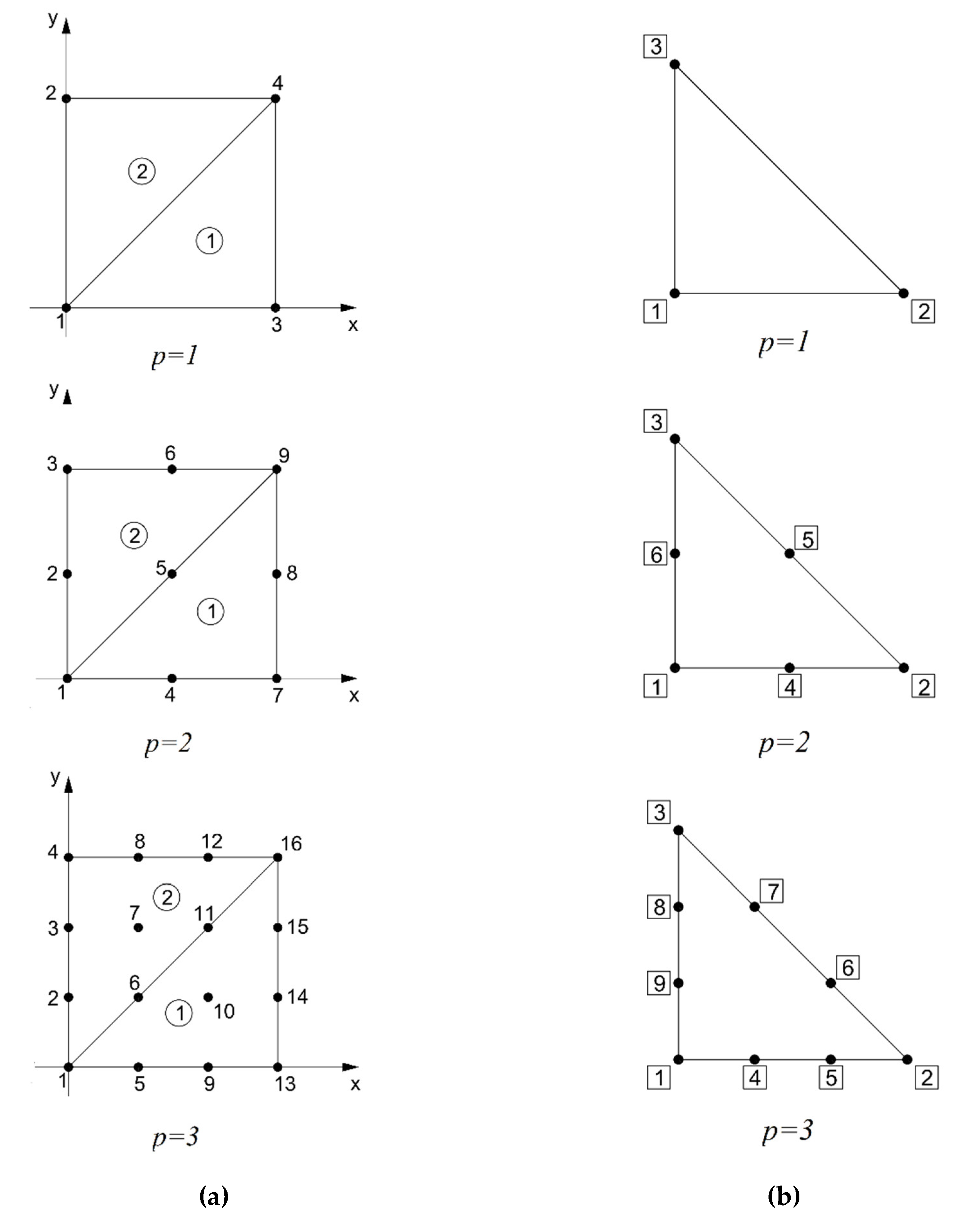
Figure 2.
Example of connectivity matrix and .
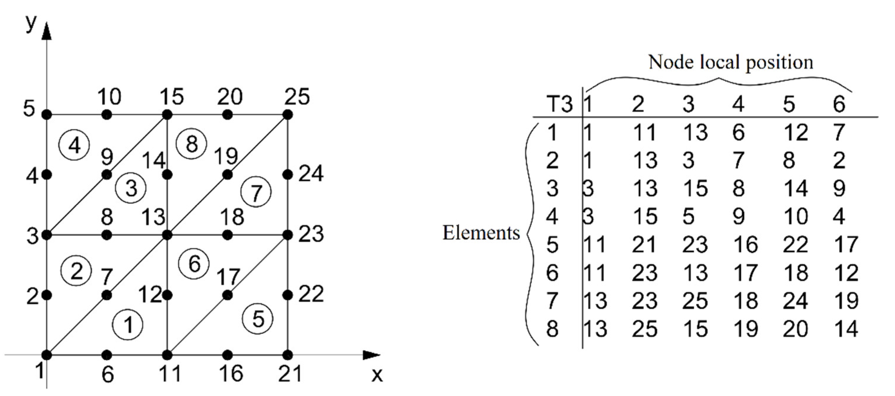
Figure 3.
Surface diagram .
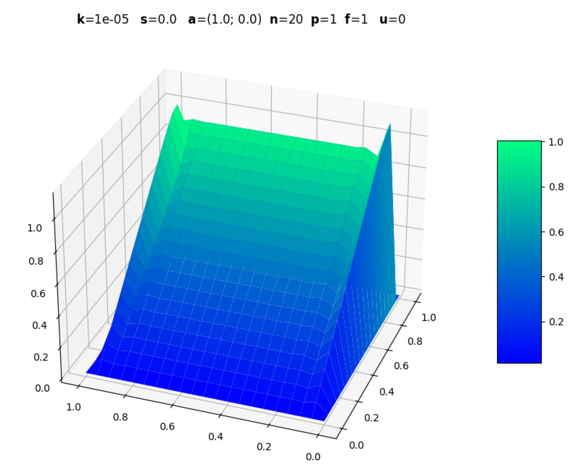
Figure 4.
Contour diagram .
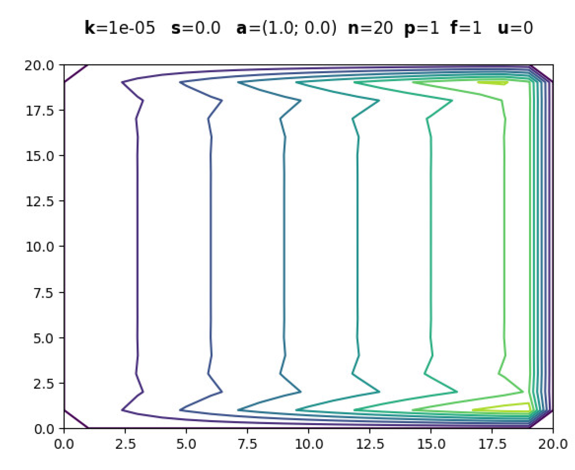
Figure 5.
Surface diagram .

Figure 6.
Contour diagram .
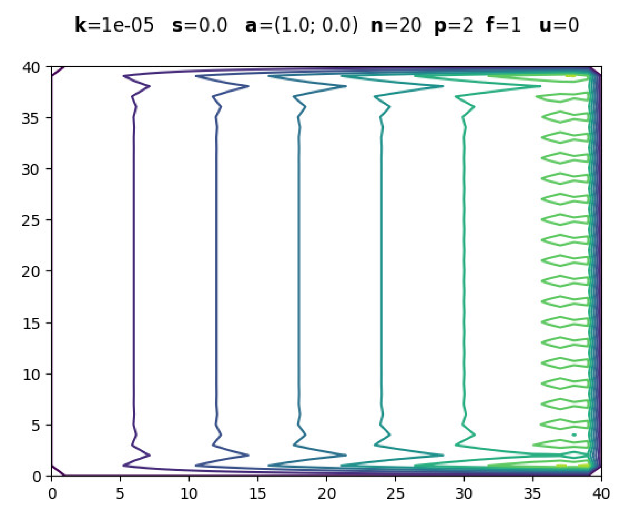
Figure 7.
Surface diagram .
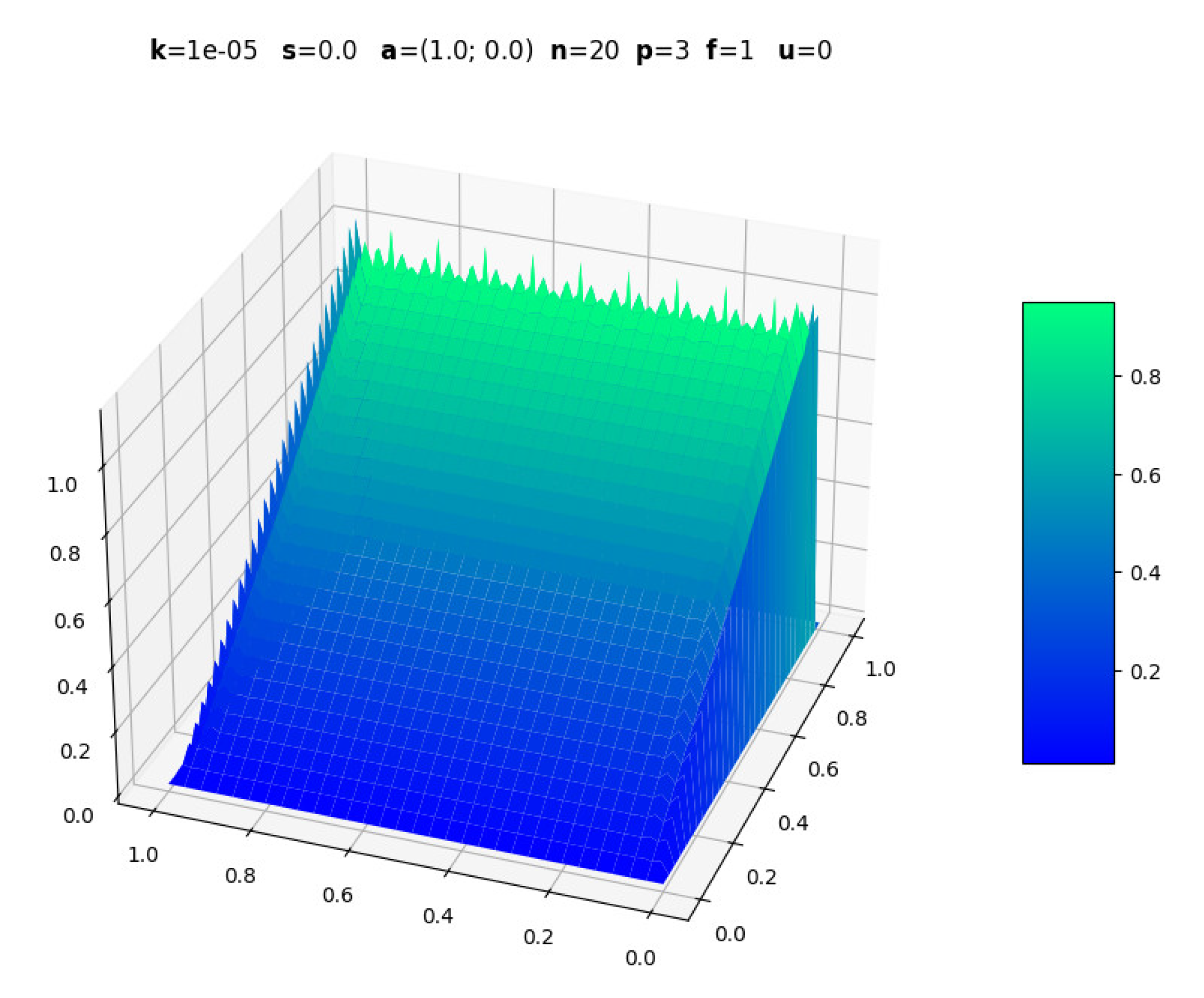
Figure 8.
Contour diagram .
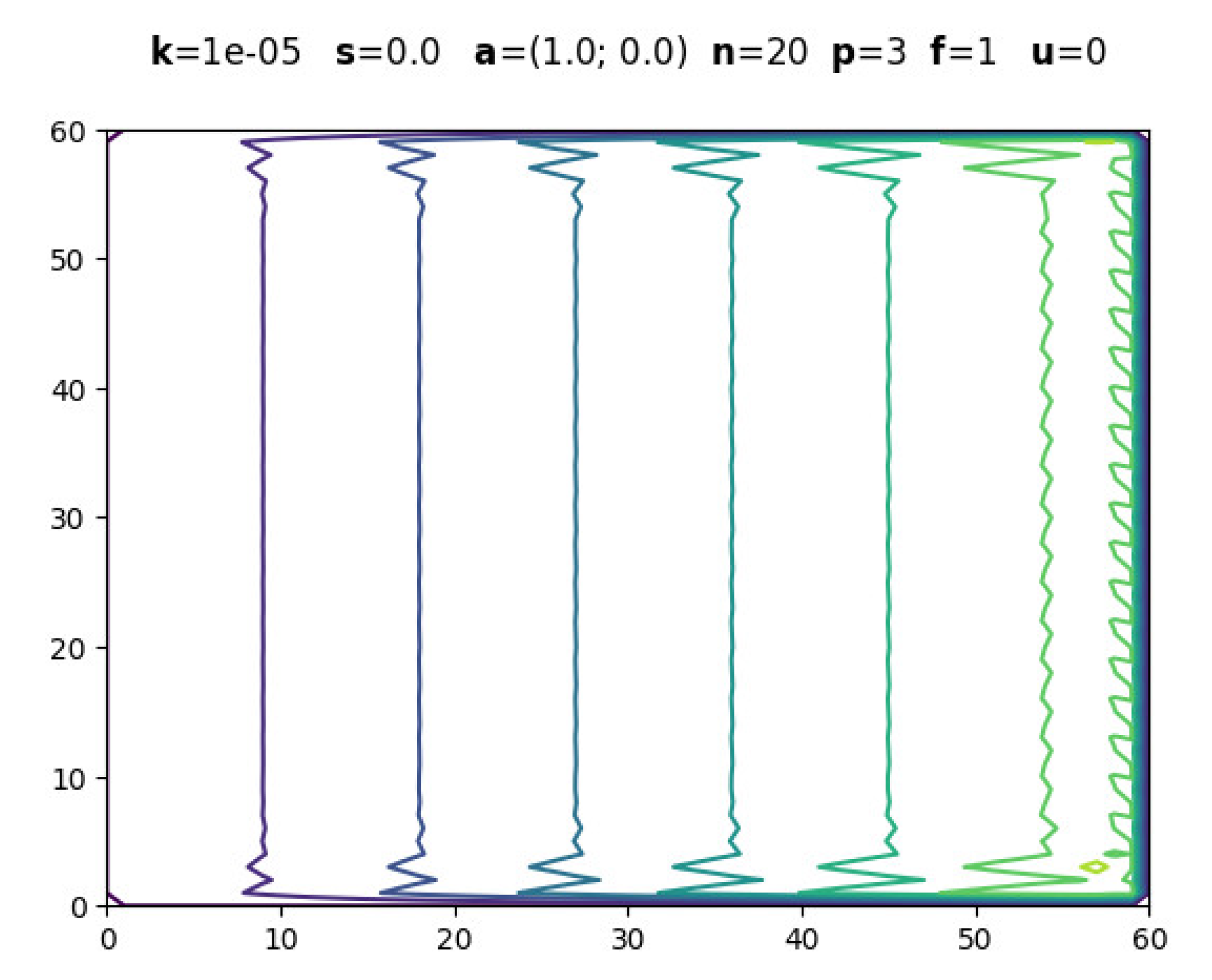
Figure 9.
Surface diagram .
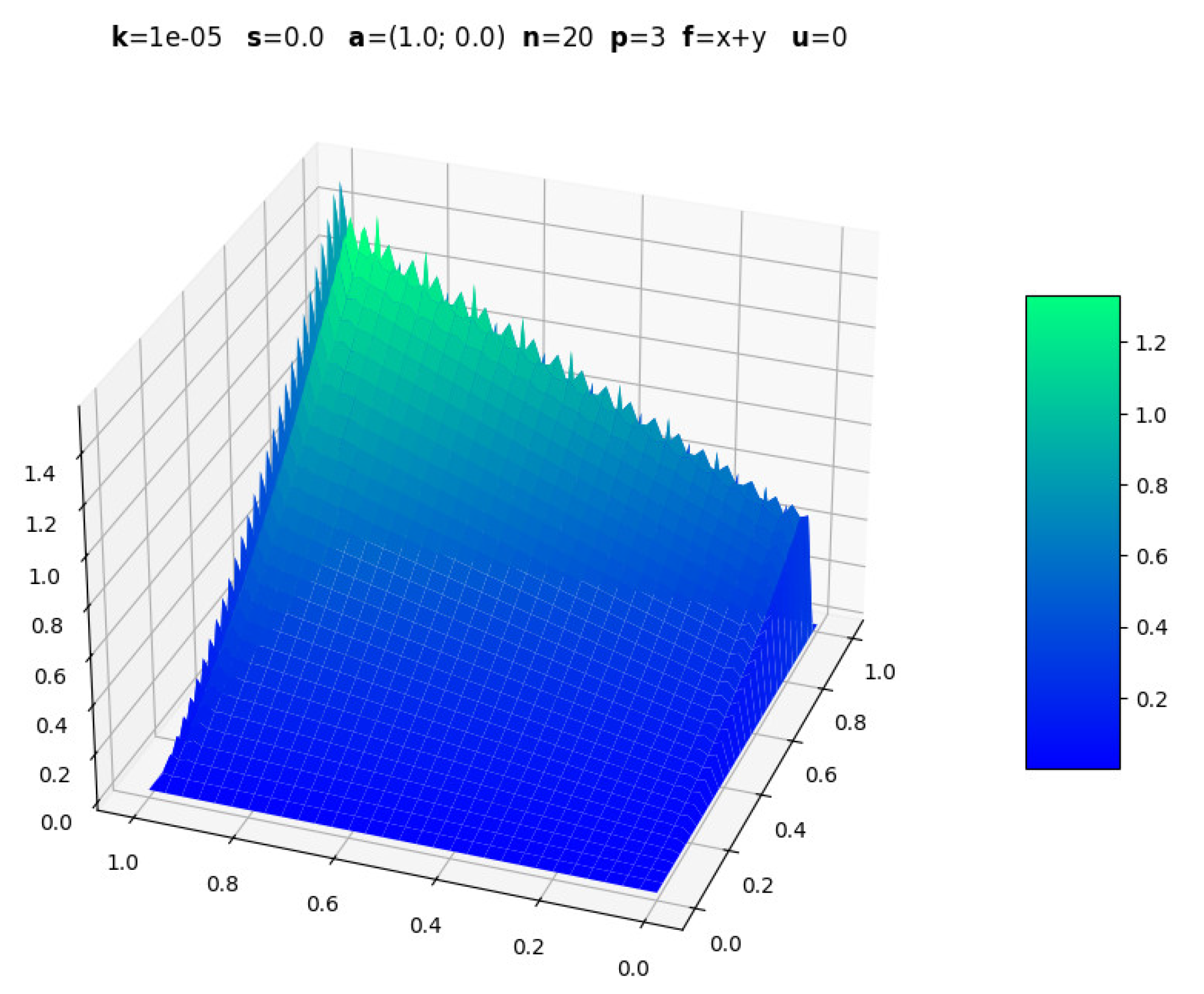
Figure 10.
Contour diagram .
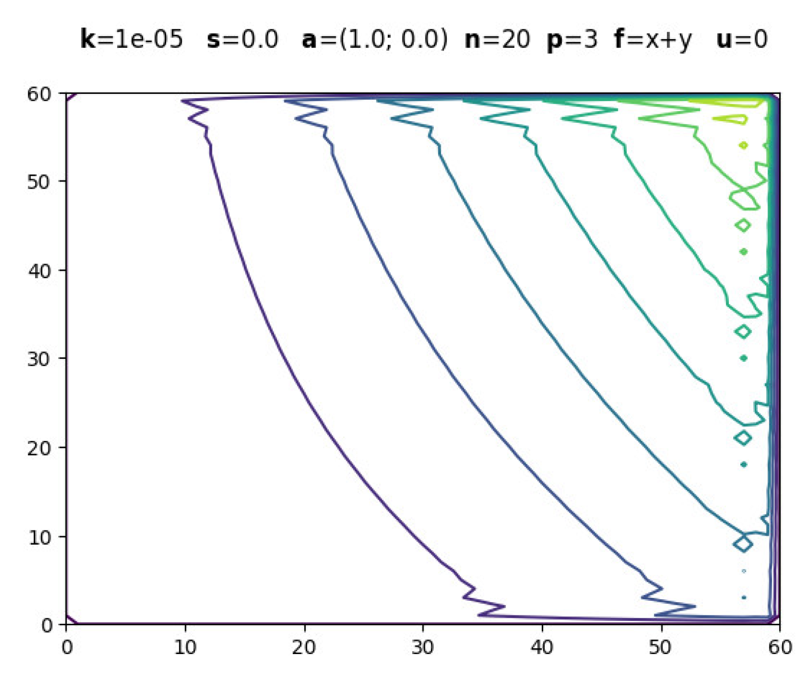
Figure 11.
Surface diagram .
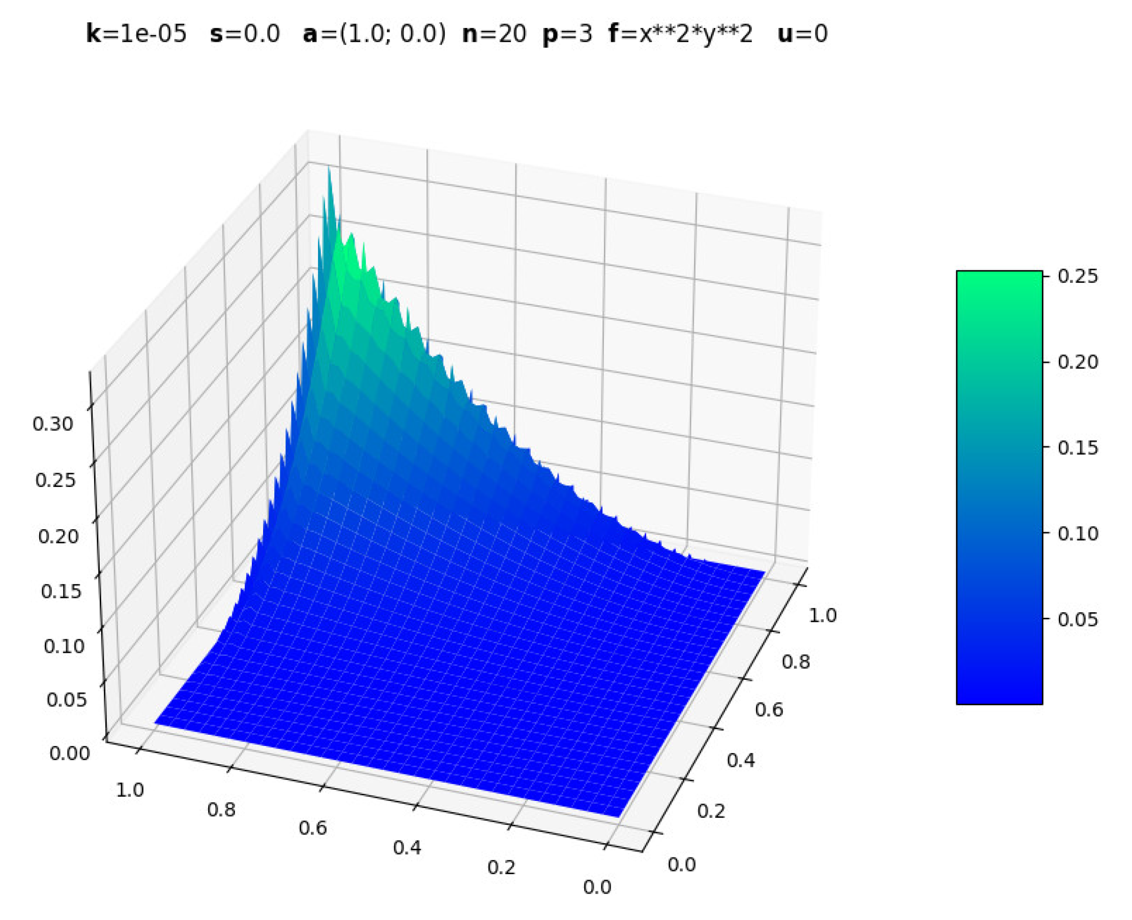
Figure 12.
Contour diagram .
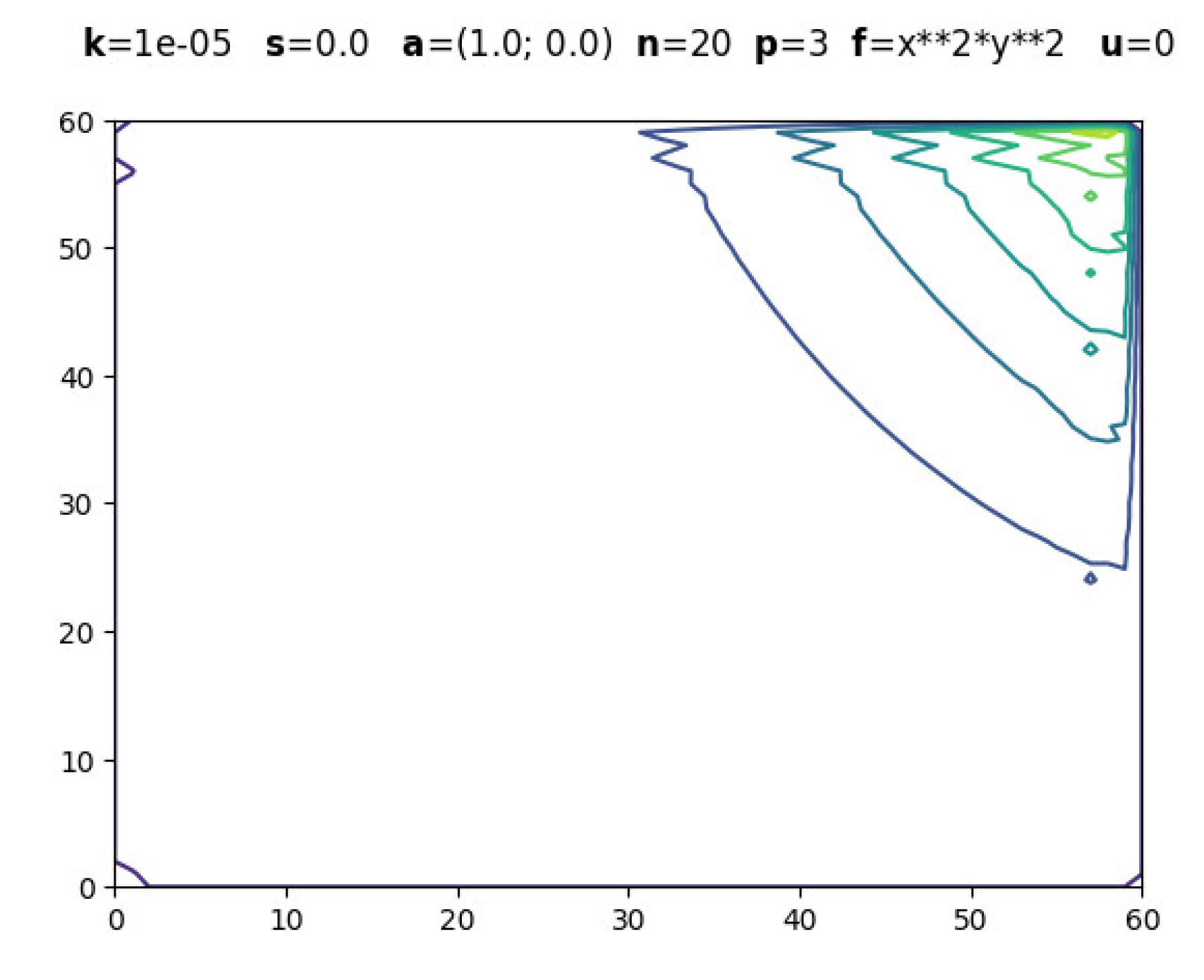
Figure 13.
Surface diagram .
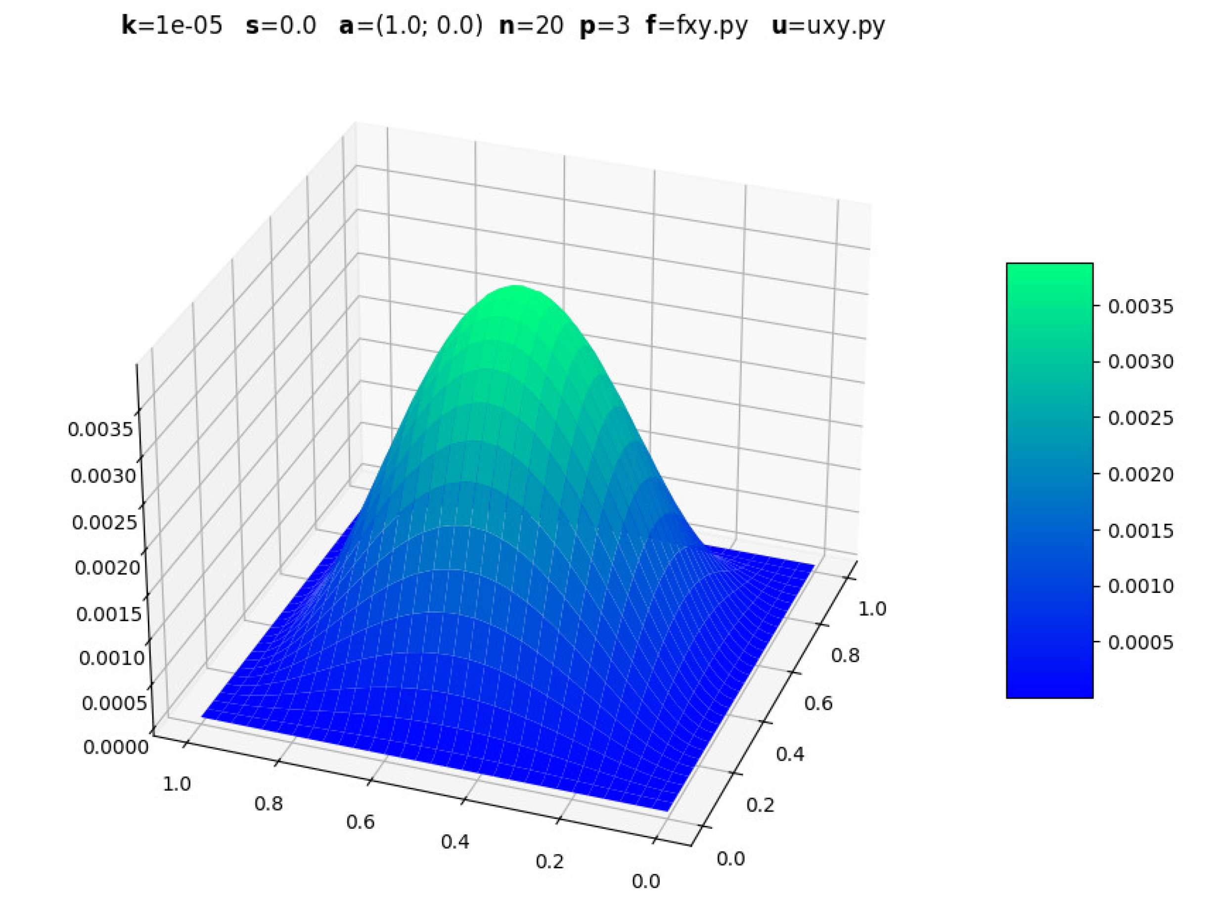
Figure 14.
Contour diagram .
Disclaimer/Publisher’s Note: The statements, opinions and data contained in all publications are solely those of the individual author(s) and contributor(s) and not of MDPI and/or the editor(s). MDPI and/or the editor(s) disclaim responsibility for any injury to people or property resulting from any ideas, methods, instructions or products referred to in the content. |
© 2025 by the authors. Licensee MDPI, Basel, Switzerland. This article is an open access article distributed under the terms and conditions of the Creative Commons Attribution (CC BY) license (http://creativecommons.org/licenses/by/4.0/).
Copyright: This open access article is published under a Creative Commons CC BY 4.0 license, which permit the free download, distribution, and reuse, provided that the author and preprint are cited in any reuse.


