Submitted:
26 June 2025
Posted:
26 June 2025
You are already at the latest version
Abstract
In addition to purely qualitative trait descriptions, biometric studies have become established within ampelography for the identification and characterisation of grapevine varieties. This publication examines the suitability of a software-assisted foliometric method, based on the self-similarity of vine leaves and employing 24 vein branching nodes, for grapevine variety identification. Various classification methods were used, including PCA, discriminant analysis, and two different neural networks. The findings show that in Vitis vinifera, leaf venation alone provides enough distinguishing features to enable an almost perfect classification of the varieties analysed here—Grüner Veltliner and its parent varieties, Traminer and St. Georgener-Rebe (Mater Veltlinis). However, due to significant individual variability, single leaves are not sufficient. By generating composite leaf data through averaging a small number of leaves, accurate classification becomes feasible. The choice of features also allows for a reasonably precise description of differences in leaf venation, which were analysed in terms of their variability across different years of data collection, within a growing season, and along the primary shoot (from proximal to distal), with particular attention to varietal differences. Leaves of the shoot middle proved more suitable for identification, while the time of year when sampling occurs is of less importance, although differences between spring and summer leaves were observed. Furthermore, the method was employed to provide a comparative description of the leaf venation patterns of the three grapevine varieties. For most traits, Grüner Veltliner exhibited intermediate characteristics between its parent varieties.
Keywords:
foliometry
; biometry
; leaf veins
; pattern recognition
; Vitis vinifera
; St. Georgener‐Rebe
; Mater Veltlinis
; Gewürztraminer
; Traminer
; Grüner Veltliner
; neural network bayesian classifier
; feed‐forward neural net
Introduction
Traditionally, grapevine variety identification has been based on the description of morphological, qualitative characteristics. In the classification and description of grapevine varieties—ampelography—leaves are generally used, as they exhibit characteristic combinations of features for each cultivar (Galet, 1990; Tassie and Blieschke, 2008; UPOV, 2008; O.I.V., 2009). Beyond purely qualitative descriptions, a number of attempts have been made to use foliometry for accurate cultivar assignment—and to investigate other aspects, such as the influence of viticultural practices on leaf morphology.
Bodor et al. (2012, 2013) compared the angles between main veins for this purpose, whereas Mancuso (1999a, 1999b, 2001, 2002) described the leaf margin as an overlay of periodic functions, adapting it using Elliptical Fourier Analysis. The resulting Fourier coefficients were then further examined using multivariate statistical methods. Alternatively, he considered the leaf margin as a fractal, i.e. a self-similar structure, and analysed its fractal parameters using multivariate techniques.
As early as 2011, Yanne et al. developed an automated identification software based on shape recognition of vine leaves. In recent years, automatic recognition software based on deep learning—particularly Convolutional Neural Networks (CNNs)—has also been developed for grapevine variety identification via leaf recognition (Taheri-Garavand et al., 2021; Terzi et al., 2024). These methods harness the impressive power of modern AI but are not without limitations. Their performance depends heavily on the amount of training data—often requiring thousands of images—and users are typically unable to determine which varietal features the neural networks use for identification. Additionally, the risk of overfitting—where the model becomes too tailored to the training data at the expense of generalisability to test data—remains a concern.
Long before artificial intelligence produced noteworthy results in pattern recognition, and prior to the availability of molecular genetic techniques for grapevine identification, attempts were made to link leaf morphology and the genetic basis of its development via algorithmic models (Lindenmayer, 1968; Bird and Hoyle, 1994). However, our understanding of how the genome shapes the phenotype remains limited to this day. Nonetheless, Lindenmayer’s 1968 approach—demonstrating how the repeated application of simple substitution rules can produce highly complex, fractal-like structures that strikingly resemble plant forms—is theoretically compelling. It highlights the remarkable discrepancy between the complexity of phenotypes and the comparatively limited data storage capacity of genomes.
The fractal nature of leaf morphology, as pointed out by Lindenmayer, was also the motivation and starting point for the development of a foliometric software tool presented by Tiefenbrunner et al. (2015). The authors developed a protocol and software for the biometric comparison of grapevine leaf venation, which has since been applied in studies of the diversity of native wild vines (Vitis sylvestris) and in comparative studies of historical cultivars, e.g. Heunisch on the slopes of the Danube, or St. Georgener-Rebe in the Pannonian region (Gangl et al., 2020; 2022). The method is based on leaf self-similarity, i.e. the quasi-fractal structure of venation.
The suitability of this method as a tool for grapevine identification, however, has not yet been systematically evaluated. This study aims to do so, using both visual comparisons based on Principal Component Analysis and separation potential assessed via Discriminant Analysis. Additionally, it investigates the potential of training various neural networks to perform variety identification using the output data from the foliometric software—using a comparatively small dataset (360 leaves).
Previous applications have not thoroughly examined or sufficiently accounted for intraspecific variation. For this reason, this study also compares the variability of leaf venation across different years of data collection, across different stages of the growing season, and along the shoot (Cousins & Prins, 2008).
This foundational “proof of principle” study is conducted by comparing the leaves of three grapevine cultivars: Grüner Veltliner and its parent varieties—Gewürztraminer and the St. Georgener-Rebe, the latter rediscovered only in 2000 (also known as Mater Veltlinis; the original name of the variety has been lost; see https://www.georgirebe.at). In addition to describing differences in leaf morphology, this study also aims to determine the rate of correct identification achieved by various neural networks.
Method
- Collection of Leaves
The method used here for the biometric analysis of leaf venation follows the paper of Tiefenbrunner et al. (2015) (see Figure 1 and Figure 2). Grape leaves of the varieties St. Georgener-Rebe, Grüner Veltliner, and Traminer were used, collected between 2022 and 2024 during the months May to September (with additional collections in April 2024 and October 2023, so not every year involved the same number of months). For each variety, nine leaves were collected each month from three primary shoots. For each shoot, one basal (proximal), one middle, and one distal leaf were selected. Occasionally, a leaf could not be used. In total, 120 leaves per variety were collected, with the attributes "variety", "year", "month", "day of year" (DOY), "position on shoot" (with the categories: proximal: p, middle: m, and distal: d), and leaf number (counted from the base of the shoot) assigned to each leaf. The number of leaves on a shoot increases throughout the year, meaning the leaf number does not precisely determine the leaf's position on the shoot. The leaves were scanned soon after being transported in a cooler or stored in a refrigerator, using a scanner (HP Scanjet G2710, HP Inc., Palo Alto, California, USA) with a uniformly blue background (blue light is efficiently used in photosynthesis and is therefore scarcely reflected by the leaves).
- Software for Recording Leaf Vein Branches; Data Collection
The selection of the branching nodes in the venation pattern was based on the property of leaf self-similarity. In Figure 1, starting from the left to right, the larger structure of the leaf can be recognised in a smaller part of it. The self-similarity is not perfect since the leaf is not truly a fractal.
The coordinates of specific leaf vein branches and vein junctions at the leaf margin were recorded. For this, a simple software was developed using the Delphi 7 Aurora IDE (Borland, Austin, Texas, USA). The image of the leaf was analysed on one half of the leaf, starting from the base of the petiole. A total of 24 vein branches or junctions were selected in a predefined sequence (1 followed by 2, and so on), and their coordinates were automatically stored (see Figure 2). However, in further analysis, the coordinates themselves were not used, as is the case in Geometric Morphometrics. The goal of biometrics is to assess the similarity of shapes (in this case, leaves). The coordinates themselves are of seemingly little value because the leaves can be rotated relative to one another and may also differ in scale. Operations that do not fundamentally change the shape include translation, rotation, and rescaling. Zelditch et al. (2004) showed that, in biometrics, coordinates ("landmarks") can be directly used for shape recognition. Traditionally, distances between points are used, and we follow this approach as it effectively eliminates the influence of translation and rotation. The software calculates the distances between the points, specifically those distances shown in Figure 2. For example, the connection between points 10 and 12, and 17 and 19 is omitted, as some cultivars may exhibit overlaps or dislocations in these areas. By omitting these points, the remaining leaf area can be accurately measured, allowing for a meaningful comparison. All 45 distances were recorded as percentages of the leaf length (with the distance between points 1 and 24 corresponding to 100%), thus avoiding problems related to scaling and ensuring better comparability. The leaf length, however, is also a valuable feature and was therefore taken into account during the analysis.
- Multivariate and Univariate Analysis; Data Evaluation
The 45 distances between branching or edge points, along with the leaf length (as the 46th feature), allow for the multivariate comparison of the leaves. As shown in Figure 2, these distances form triangles whose areas can be calculated using Heron's formula. This also enables the calculation and univariate comparison of the areas of the highlighted leaf sectors (I to IV in Figure 2). Furthermore, using the law of cosines, the base angles of these areas can be determined. The leaf length was also an additional target for univariate analysis.
For the univariate statistics, Statgraphics™ Centurion XV (Statpoint Inc., Herndon, Virginia, USA) was used, complemented by own software for the Random-Resample Rank Test (for a nonparametric multiple comparison of medians). Various methods for comparing means (ANOVA, multiple mean comparison, and the nonparametric Kruskal-Wallis test) were performed, along with methods to check the assumptions of the tests (particularly the Levene test for examining variance homogeneity). The following properties were compared: variety, position on the shoot, season, and year.
Multivariate Statistics: Principal Component Analysis (PCA) was conducted using the ViDaX software (LMS-Data, Munich – Trofaiach) for the representation of leaf similarity. This also allowed the investigation of whether composite leaves (with features whose values correspond to the averages of multiple leaves) are more suitable for clustering than the original leaves. To analyse which leaf features (distances and length) are relevant for varietal differences, the PCA option in Statgraphics was used, as it is more suited for this purpose. For classification (e.g. to the variety), Discriminant Analysis was performed, and the Neural-Network-Bayesian-Classifier (Statgraphics), which offers a relatively high resilience against "overfitting", was also employed. The results from these two methods were compared with those of a classic "Feed-Forward" network provided by ViDaX. Due to the small size of the training data (16,560 individual data points), the "Jackknife" procedure was applied: the training is conducted with all leaves except one, which is then classified by the trained network. This process was repeated for all leaves, and the rate of correct classifications was determined.
Results and Discussion
In the ampelography of the St. Georgener-Rebe, Regner (2013) describes the shoot tip, shoot orientation, characteristics of the grape shape, berry shape, colour, weight, comparative ripening time, and berry flavour, as well as features of the leaf. Regarding the latter, it is worth mentioning that the leaf margin, where the veins meet, is sharply serrated and forms an acute angle (Gangl et al., 2022).
In contrast, for Traminer, the leaf margin at the vein terminations is generally more rounded compared to the St. Georgener-Rebe, and the leaf shape is less acute. This also applies to the lobing. Furthermore, the leaf is often less lobed, meaning the sinus between the lobes is shallower, giving the leaf a more circular overall appearance.
The Grüner Veltliner, in these respects, is more intermediate. However, individual differences between the leaves are quite significant. “Typical” leaves of the three varieties are shown in Figure 3. A multivariate comparison of 360 leaves to the pattern of leaf venation using PCA (with only two dimensions, or three if symbol size is considered) shows that the varieties are not well-separated (also Figure 3). It thus raises the question of whether it is even possible to reliably assign leaves to the three varieties. Still, the corresponding clusters of the varieties are not entirely overlapping; they are slightly shifted from each other, suggesting that such identification might be possible.
Variety Identification and Separability
To reduce the coefficient of variation and eliminate outliers, the data from multiple leaves can be combined by calculating the average for each feature. These "composite leaves" can then be compared again using PCA. Without further knowledge of whether certain leaves might be more suited to represent a variety than others, it is sensible to randomly select the leaves to be combined. This "mixing" was performed with appropriate own software, where only the number of leaves combined into each composite was varied. Ten composites were created for each variety from the 120 real leaves, and the resulting composites were compared using PCA (Figure 4).
As shown in the figure, separability improves significantly with the creation of composites, even when the number of leaves per composite is still relatively low. The subfigure in the top-left corner uses the original leaves, but only ten per variety (compared to the 120 shown in Figure 3), and, as expected, there is substantial overlap. Already with five leaves per composite, the situation changes, and clear clusters start to form. The clustering quality improves slowly with the increasing number of leaves per composite, but after 25 leaves, a degree of separation along the first principal component (PC1; x-axis) is achieved. The second principal component (PC2; y-axis) primarily allows for separating the parent varieties from their offspring, but along PC1, the offspring lies between the two parents, meaning that the Grüner Veltliner still, in terms of its leaf characteristics, blends traits from both of its parents. To verify whether this holds universally, it would be worthwhile to study other comparable parent-offspring triplets, such as Zweigelt with its parents St. Laurent and Blaufränkisch.
One issue with the method described above is that a leaf may be part of multiple composite leaves. In a population of 120 leaves per variety, this might still be a minor issue when there are five leaves per composite and ten composites per variety (random sampling of 50 leaves from 120), but this becomes more significant when there are 25 leaves per composite. "Without replacement," 10 composites of 12 leaves each can be created from 120 leaves. These can then be compared with the corresponding amount of composites created by randomly selecting 12 leaves "with replacement." A potential result is shown in Figure 5.
In this example, it is apparent that whether composites are created "with" or "without replacement" plays a role. It then raises the question of how this might affect classification techniques, specifically in terms of correct assignment of leaves to varieties.
Leaf Venation and Variety Recognition
To investigate the separability of the leaves and their assignment to varieties, a discriminant analysis was conducted. This method generates discriminant functions, which help assign the variety based on the 46 metrics and can be visualised as dimensions. The two functions used as axes in Figure 6 are statistically significant in their discriminative power (P=0.0 in all cases) and are relevant. Using the original data (120 leaves per variety), a reasonably good separation is obtained: the correctness of assignment is 91.36% (where a random assignment would expect 33.33%), and it is nearly equal for all three varieties (slightly better for the Traminer). By forming 100 composites per variety, each consisting of 10 leaves, the correctness of assignment can be increased to 100% (shown on the right side of Figure 6). However, this result must be considered with caution because more objects than features are required for the discriminant analysis, and, as mentioned before, many composites contain data from the same leaf.
A practical application for this method would be to compare a pre-existing training set, created in previous years, with a composite of several leaves for classification purposes. Creating 100 or more composites, however, seems unrealistic. To work with fewer composites, different classification methods than discriminant analysis would be needed.
The Neural Network Bayesian Classifier from Statgraphics does not separate the original data (the 360 leaves) as well as discriminant analysis. Only 77.44% are correctly assigned (expected under the assumption of random assignment: 33.33%). Interestingly, the Grüner Veltliner variety is almost equally often confused with the other two varieties (11 as St. Georgener-Rebe and 12 as Traminer), while the other two varieties are much more frequently mistaken for the Grüner Veltliner than for its other parental variety (of StG, 23 are classified as GV and only two as Tr; of Tr, 29 are mistakenly classified as GV and four as StG). This may be a consequence of the existing relationships, an assumption that should, as mentioned, be tested with more parental-offspring variety triplets.
If one forms 100 composites per variety, each consisting of ten leaves, the correct classification increases to 99.67% (one Gewürztraminer is mistakenly classified as a Grüner Veltliner). The method can now be applied to fewer objects (leaves or composites) than there are features. If ten leaves (i.e., no composites) are selected per variety, the correct classification rate is 73.33%, which is comparable to the performance of separating 120 leaves per variety. However, ten composites consisting of five leaves each already achieve 100% variety recognition, and this of course does not change even if more, up to 25 leaves per composite, are used (the number of leaves per composite is increased in steps of five). If one ensures that each leaf is only present in one composite (without replacement, resulting in ten composites per variety, each consisting of twelve leaves), the classification quality is 96.67% (one St. Georgener-Rebe composite is classified as Grüner Veltliner), which is also very good and, of course, much better than the individual leaf classification.
The "Neuronal Recognition" with the Feed-Forward Network from ViDaX, trained using backpropagation with the Jackknife method, yields a correct recognition of 84.10% of the leaves for the original data (360 leaves), which is better than the performance of the Neural Network Bayesian Classifier and worse than that of the discriminant analysis. The wrongly assigned Grüner Veltliner leaves are found about equally often in both parental varieties (for GV: StG=10; Tr=12), while St. Georgener-Rebe and Traminer are significantly more often confused with Grüner Veltliner than with the other parental variety (for StG: GV=15; Tr=3, for Tr: GV=14; StG=3).
Reducing the number of leaves per variety to ten (instead of 120) results in a correct recognition rate of 90%, which is even slightly higher, although the exact percentage obviously depends on the randomly selected leaves.
For 100 composites, each consisting of ten leaves, the correct assignment rises to 100%, just as with discriminant analysis. Reducing the number of composites to ten, five leaves per composite already results in 96.7% correct assignment to a variety (one composite from a set of 30 is incorrectly assigned). Increasing the number of leaves per composite in steps of five, one finds 100% correct recognition starting at ten leaves per composite, even if it is ensured that each leaf only appears in one composite (without replacement).
In summary, while discriminant analysis provides the best separation of the original data, neural networks have an advantage when using composites. Individual leaves often differ greatly, even when belonging to the same variety, and even moderately sized composites, e.g., consisting of five leaves, already offer a clear advantage here. In working with these, however, neural networks are beneficial due to their greater flexibility regarding the object-feature relationship.
- Selection of Leaves
In addition to the variety, for each leaf the collection time (season and year) as well as its position on the shoot were documented. It is possible that one of these attributes influences the suitability for variety classification. The position on the shoot is recorded both as a metric and discrete characteristic by the node, counted from the base at which it is inserted (= the leaf number), and also as an ordinal characteristic, with three categories distinguished during sampling: basal or proximal (p), middle (m), and distal (d: towards the shoot tip). To investigate the importance of the leaf's position on the shoot for the quality of the classification, the ordinal characteristic was used. First, composite leaves were created consisting of: all leaves of a variety (3 composites); all leaves of a variety and their shoot position (9 composites); all leaves of a variety, from one year, and one shoot position (27 composites). These are presented in three graphs (PCAs), each summarising the composites of one position (p, m, d), and additionally showing the position of the composites from all leaves of a variety (Figure 7). It can be seen that the composites from the middle of the shoot (m) cluster better, i.e., are more similar to each other than those from the shoot base or tip. It therefore seems more advantageous for variety classification to use only leaves from the middle of the shoot.
This can also be shown in another way. The "Jackknife" protocol for ViDaX’s neural network provides information for each individual object (in this case, the 360 leaves are the objects) on whether it was correctly assigned (in this case: to the variety). It shows that middle leaves are assigned correctly 88.24% of the time, proximal leaves only 81.70%, and distal leaves just 80.83%. If the two neural networks are sorting not by variety but by shoot position, the correctness is relatively low (56% instead of the expected 33% for Statgraphics and 64.4% for ViDaX), but it can be observed that misclassifications mostly occur with adjacent positions. This suggests that there is a morphological gradient along the shoot, though this will not be explored further here (except for leaf length).
In a similar manner, the importance of the collection time throughout the year for variety recognition can be examined. In the PCAs of Figure 8, composites are again used, which, separated by variety, contain all leaves from a particular time period (left sub-figure). The collection season was divided into three equal intervals (I: end of April to end of June, II: to mid/end of August, III: to mid-October). This results in three composites per variety. A fourth composite includes all leaves from a variety (I-III). It can be seen in Figure 8 (left) that the season is split by the latter in such a way that season period I is separated from the rest of the year, and for all three varieties, higher values are reached for PC2 (y-axis; ordinate) than for the other two intervals.
This fact, as well as the similar trend across all varieties, suggests that a morphological change in the leaves occurs throughout the year. Even when dividing the season into months (right figure), this is confirmed, with the transition occurring in the composite containing all leaves of a variety (4-10) at the point between June and July. Roughly speaking, one can talk about a spring and a summer/early autumn leaf morphology. The specific differences between the two were not further investigated.
The "Jackknife" protocol of the ViDaX network allows determining how many leaves collected in a given month were correctly assigned to the variety. The recognition rate is notably low only for April (59.26%). However, vine development in 2024 was the only year advanced enough to allow for early leaf collection. For all other months, the correct variety recognition ranged from 80.68% (August) to 92.59% (May). It cannot be said that classification quality improves or worsens over the course of the year. The recognition quality for the month in which a leaf was collected lies, depending on the network, between about 24% (Statgraphics) and 29% (ViDaX), which is higher than random assignment (14.28%), but still low. In summary, it can be said that for variety classification, one should not collect leaves too early in the year, but otherwise, the timing plays a minimal role. Perhaps it would be beneficial to collect leaves twice: once in spring and once in summer.
The correct assignment to the collection year (2022-2024) is achieved at about 50% (expected: 33.33%).
Leaf Shape in Variety Comparison
Using a well-separating PCA (e.g., Figure 4, bottom right), one can investigate which characteristics are important for high-quality separation of varieties, as for each principal component (PC axes in the figure), there exists a constant for each characteristic, whose value also determines the position along the axis. Characteristics with a high absolute value are more important than others, which, in the case of clear separation of varieties along an axis, means that these characteristics are significant for variety classification. In the mentioned figure, PC1 separates the two parental varieties from each other, while PC2 separates them from the offspring Grüner Veltliner. It is also helpful to examine the medians of the segment lengths in the variety comparison. The result of this analysis is summarised in Figure 9: the leaf areas important for variety separation are highlighted in colour.
For Traminer, these areas are located in the leaf sectors marked with Roman numerals in Figure 2, forming the basal sections of sectors III and IV, as well as an additional area near the leaf base in sector II. Here, the segments are on average relatively longer than in the other two varieties. For the St. Georgener-Rebe, this applies to sector I, as well as the distal (tip) areas of leaf sectors II to IV. Since Grüner Veltliner generally falls between its parental varieties for most characteristics, there is only one leaf area where it significantly differs from the other varieties. This is the leaf base, i.e., an approximately triangular section from the leaf insertion point 1 (see Figure 2) to point 6 of sector II, and from there to the origin of sector III (point 11) and IV (point 18).
A characteristic that can be compared well is leaf length (Figure 10).
With an average length of 6.8 cm, Traminer has the shortest leaves. Grüner Veltliner lies between the parental varieties with a leaf length of 8.9 cm. The leaves of the St. Georgener-Rebe are, on average, 12.4 cm long. The differences are significant (Kruskal-Wallis test p=0.0; the samples are not normally distributed). In all varieties, the middle leaves are longer than the proximal or distal ones near the shoot tip. According to the Random-Resample Rank test, the difference is significant for all comparisons, except for those between intra-varietal comparisons of proximal and distal leaves and middle and proximal leaves for Traminer.
The development of leaf length was examined using linear regression, separated by variety and shoot position (not shown). In all three varieties, leaf length increases over the course of the season, but only slightly for the middle leaves (and not at all for Traminer). For Traminer and Grüner Veltliner, the proximal leaves exhibit the greatest increase (k=0.015, R=0.53 and k=0.02, R=0.14, respectively). For the St. Georgener grape, however, it is the distal leaves that grow the most (k=0.03, R=0.47). The correlation between DOY (day of year) and leaf length is, however, very low in all cases, and only the consistency of the trends across the varieties suggests that the increase in length over the season is a real phenomenon.
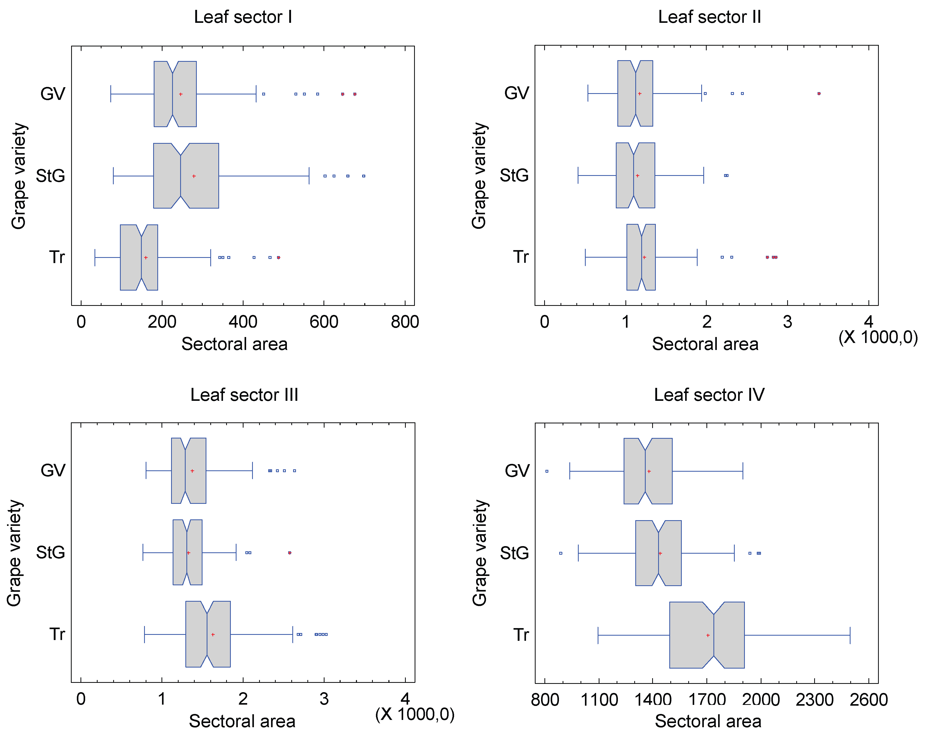
With the leaf length-scaled data, the relative area for sectors I to IV was calculated and compared across varieties (Figure 11). For leaf sector I, a significant difference in area exists between all varieties (Kruskal-Wallis test p=0.0, multiple means comparison). The largest relative area in sector I is found for the St. Georgener-Rebe, with Grüner Veltliner reaching 88.39% of its leaf area, and Traminer 57.36%. For sector II, no significant differences are found between the varieties, in contrast to sector III, where Traminer significantly differs from the other varieties (Kruskal-Wallis test p=0.0, multiple means comparison). Compared to this variety, the St. Georgener-Rebe only occupies 81.59% of the area in this sector, with Grüner Veltliner in between at 84.28%. However, the difference between the latter two varieties is not significant. The difference in leaf area between all varieties in sector IV is very pronounced (Kruskal-Wallis test p=0.0, multiple means comparison). Here again, Traminer has the largest relative leaf area. Compared to Traminer, the St. Georgener-Rebe has only 84.29% of the area, and Grüner Veltliner 80.78%. Grüner Veltliner, which significantly differs from both parental varieties, does not fall between the others for this characteristic.
The opening angle α of the sectors was also investigated. Again, significant differences emerge. For sector I, with an angle of 50.31°, Grüner Veltliner has an angle about three degrees larger than the other varieties. In sector II, there is no significant difference between the varieties (the angle lies between 57° and 59°), while in the third leaf area, Traminer's angle of 37.89° is about 2° larger than the others. In sector IV, αIV is largest for Traminer at 38.46°. However, the difference is not very large, only around 2°. The sum of the angles αI to αIV is largest for Grüner Veltliner, at 181.65°. This suggests the most overlap at the leaf base (as must occur with more than 180° per leaf half), with the least overlap for the St. Georgener-Rebe.
In conclusion, the results show that for Vitis vinifera, leaf venation alone provides enough characteristics to enable almost perfect classification of the varieties studied here. However, due to the large individual differences, a single leaf is not sufficient for this. By averaging across multiple leaves for all characteristics, thus reducing the coefficient of variation and eliminating outliers, this is achievable. The choice of characteristics also allows a good description of the differences in leaf venation. A disadvantage of the presented procedure is that it cannot be directly applied to other dicotyledonous plant species as the leaf vein pattern is highly variable between them.
References
- Bird, R.J. and Hoyle, F., On the shape of leaves. J. Morphol. 219: 225-241, 1994.
- Bodor, P., Baranyai, L., Balo, B., Toth, E., Strever, A., Hunter, J.J. and Bisztray, G.D., GRA.LE.D. (Grapevine Leaf Digitalitzation) software for the detection and graphic reconstruction of ampelometric differences between Vitis leaves. S. A. J. Enol. Vitic. 33(1): 1-6, 2012.
- Bodor, P., Baranyai, L., Ladanyi, M., Balo, B., Strever, A., Bisztray, G.D. and Hunter, J.J., Stability of ampelometric characteristic of Vitis vinifera L. cv. ‘Syrah’ and ‘Sauvignon blanc’ leaves: Impact of within-vineyard variability and pruning method/bud load. S.A. J. Enol. Vitic. 34(1): 129-137, 2013.
- Cousins, P. Cousins, P., Prins, B., Vitis Shoots Show Reversible Change in Leaf Shape along the Shoot Axis. Proceedings of the 2nd Annual National Viticulture Research Conference, July 9–11, 2008.
- Galet, P., French grapevine varieties and vineyards. The French ampelography, vol. 2. - Montpellier, 1990.
- Gangl, H., Tscheik, G., Leitner, G., Probst, A., Tiefenbrunner, W., Die „St. Georgen-Rebe“: Entwicklung im Jahresverlauf, Biometrie und Aromakomposition des Weines. Mitteilungen Klosterneuburg 72, 204-221, 2022.
- IPGRI, UPOV, OIV, Descriptors for Grapevine (Vitis spp.). International Union for the Protection of New Varieties of Plants, Geneva, Swizerland, 1997.
- Lindenmayer, A., Mathematical models for cellular interaction in development. J. Theoret. Biol. 18: 280-315, 1968.
- Mancuso, S., Elliptic Fourier Analysis (EFA) and Artificial Neural Networks (ANNs) for the identification of grapevine (Vitis vinifera L.) genotypes. Vitis 38(2): 73-77, 1999a.
- Mancuso, S., Fractal geometry-based image analysis of grapevine leaves using the box counting algorithm. Vitis 38(3): 97-100, 1999b.
- Mancuso, S., Clustering of grapevine (Vitis vinifera L.) genotypes with Kohonen neural networks. Vitis 40(2): 59-63, 2001.
- Mancuso, S., Discrimination of grapevine (Vitis vinifera L.) leaf shape by fractal spectrum. Vitis 41 (3): 137-142, 2002.
- Regner, F., Ampelografische Beschreibung der Sorte ‘St. Georgen’, in: St. Georgen – Heimat der Veltliner Ur-Rebe. Dorfblick St. Georgen (Hrsg.), 333, 2013.
- Taheri-Garavand, A.; Fanourakis, D.; Zhang, Y.-D.; Nikoloudakis, N. Automated Grapevine Cultivar Identification via Leaf Imaging and Deep Convolutional Neural Networks: A Proof-of-Concept Study Employing Primary Iranian Varieties. Plants 10, 1628, 2021. https:// doi.org/10.3390/plants10081628.
- Tassie, L. and Blieschke, N., Ampelography: do you know what variety you are planting in your vineyard or nursery. Austr. NZ Grapegrower Winemaker (537): 31, 2008.
- O.I.V. 2nd edition of the OIV descriptor list for grape varieties and Vitis species. 2009. (http://www. oiv.int).
- Terzi, I. Terzi, I., Ozguven, M. M., Yagci, A., Automatic detection of grape varieties with the newly proposed CNN model using ampelographic characteristics, Scientia Horticulturae, 334, 113340, 2024. ISSN 0304-4238, https://doi.org/10.1016/j.scienta.2024.113340. (https://www.sciencedirect.com/science/article/pii/S0304423824004977).
- Tiefenbrunner, D., Gangl, H., Leitner, G., Tiefenbrunner, W., Blattgestalt und – vielfalt bei der Wilden Weinrebe (Vitis vinifera ssp. sylvestris) der March- und Donauauen im Vergleich zur Kulturrebe. Mitteilungen Klosterneuburg 65: 143-156, 2015.
- UPOV: Guidelines for the conduct of test fur distinctness, uniformity and stability TG 50/9. - Geneva Switzerland, 2008. http://www.upov. int/edocs/tgdocs/en/tg050.pdf.
- Yanne, P., Zhang, J. and Li, H., Automatic grape varieties identification by computer. Bull. OIV 84(959/960/961): 5-14, 2011.
- Zdunic, G., Maul, E., Eiras Dias, J.E., Munoz Organero, G., Carka, F., Maletic, E., Savvides, S., Jahnke, G.G., Nagy, Z.A., Nikolic, D., Ivanisevic, D., Beleski, K., Maras, V., Mugosa, M., Kodzulovic, V., Radic, T., Hancevic, K., Mucalo, A., Luksic, K., Butorac, L., Maggioni, L., Schneider, A., Schreiber, T., Lacombe, T., Guiding principles for identification, evaluation and conservation of Vitis vinifera L. ssp. Sylvestris. Vitis 56, 127-131, 2017.
- Zelditch, M.L., Swiderski, D.L., Sheets, H.D., Fink, W.L., Geometric Morphometrics for Biologists: A primer. Elsevier, 2004.
Figure 1.
Self-similarity in a vine leaf – The whole is reflected in the part. By reducing in size and rotating, the red area can be transferred into the green, which then transforms into the blue and eventually the yellow. A vine leaf exhibits four levels of self-similarity (occasionally one more). However, the self-similarity is not perfect. According to Tiefenbrunner et al. 2015, modified.
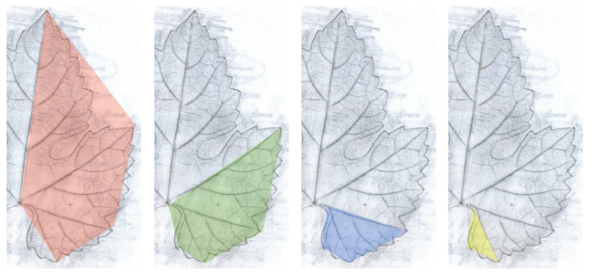
Figure 2.
Procedure of the foliometric analysis. The 24 nodes are 'clicked' in the prescribed sequence, and the 45 segments are calculated. For areas I to IV, see the main text. For better visibility of the veins, a drawing was used here, which was created by placing a vine leaf between a hard, flat, smooth surface and tracing paper, then gently and lightly rubbing over the paper with a soft pencil. According to Tiefenbrunner et al. 2015, modified.
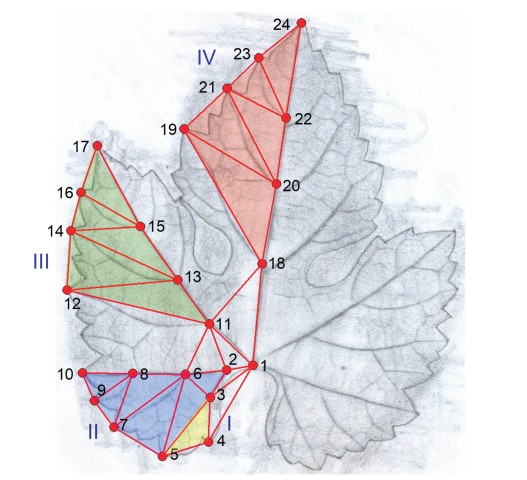
Figure 3.
Shown are more or less typical leaves for the three varieties (top). The Grüner Veltliner is intermediate, in terms of leaf margin and lobing, between its parent varieties. The high degree of variability within the varieties can be observed—regarding leaf venation—by the strong overlap in the three-dimensional PCA (below; the third dimension is indicated by the symbol size). In each subfigure, one variety is highlighted in colour and by symbol size.
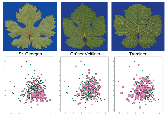
Figure 4.
Composite leaves of the three varieties in comparison. The number in the top-left or bottom-left corner of each subfigure indicates how many real leaves were used to create a composite leaf (by averaging each of the 46 traits). A 3D PCA is shown.
Figure 4.
Composite leaves of the three varieties in comparison. The number in the top-left or bottom-left corner of each subfigure indicates how many real leaves were used to create a composite leaf (by averaging each of the 46 traits). A 3D PCA is shown.
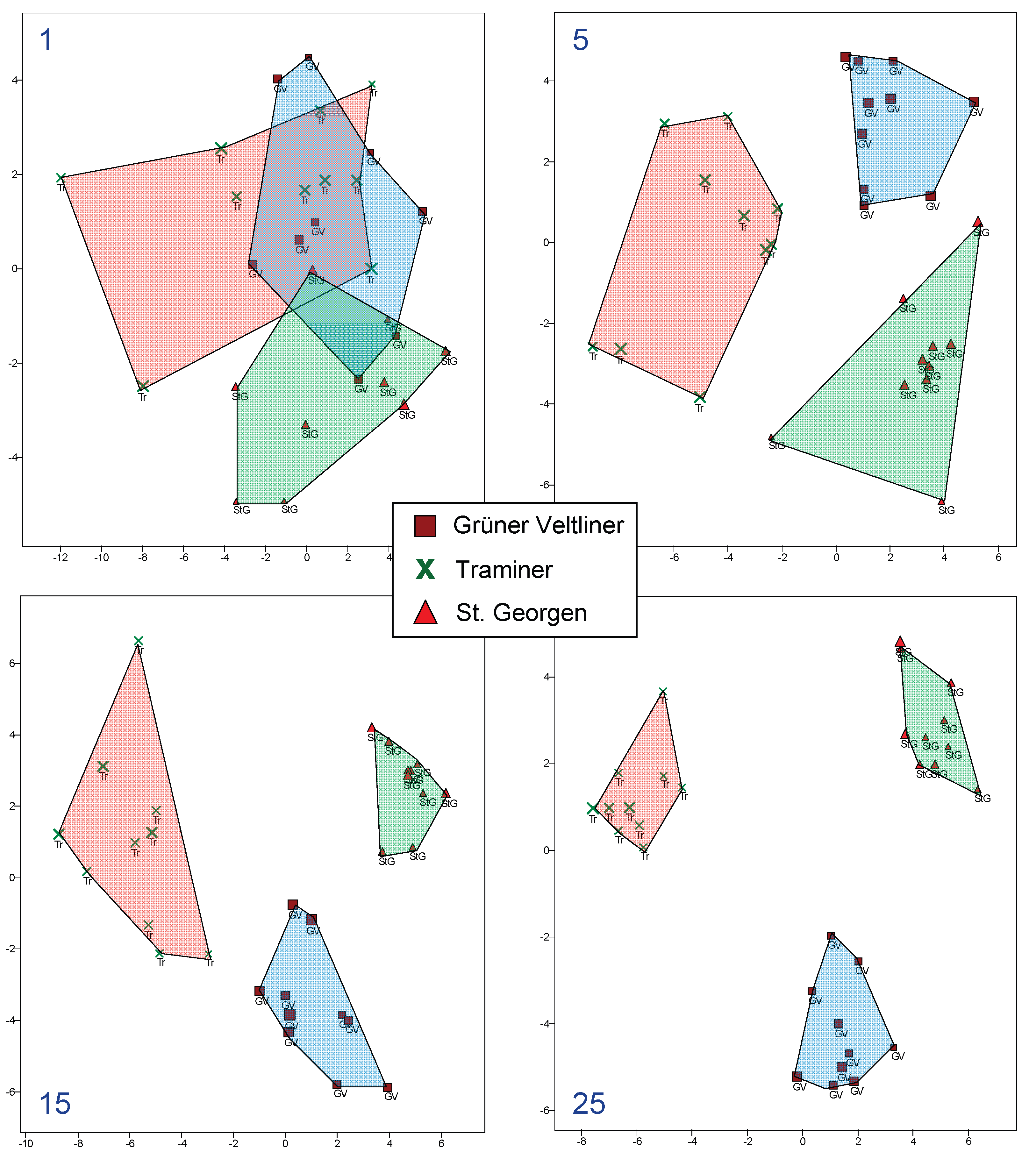
Figure 5.
Composites of the three varieties made from five leaves each, left: with, right: without replacement. On the left, a leaf can be part of several composites, whereas on the right, it cannot.
Figure 5.
Composites of the three varieties made from five leaves each, left: with, right: without replacement. On the left, a leaf can be part of several composites, whereas on the right, it cannot.
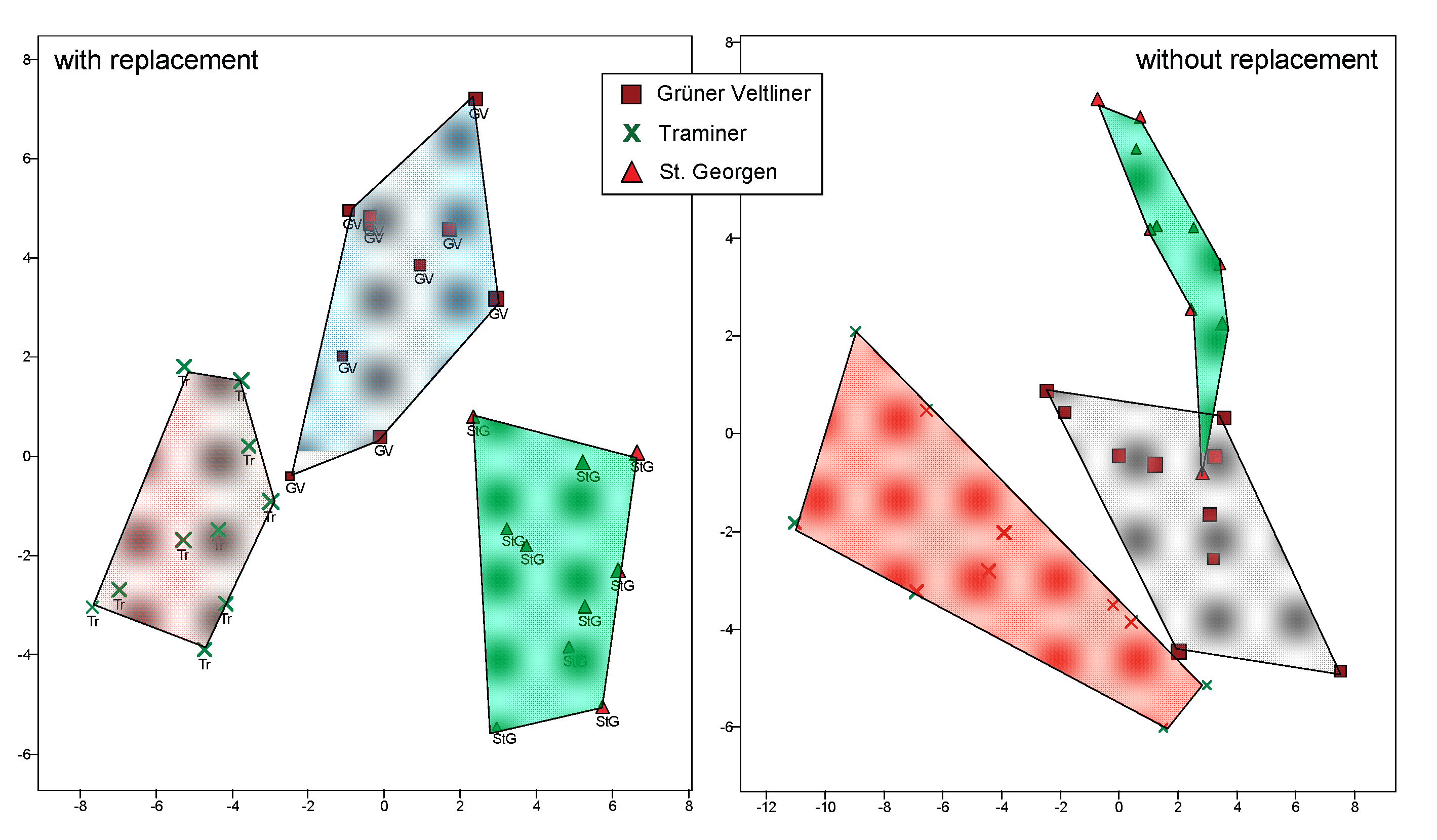
Figure 6.
Discriminant analysis and representation of the leaves as points, whose coordinates are determined by the two significant separation functions of the method. Left: Original data (120 points per variety); right: for each variety, 100 composites were created from ten randomly selected leaves. The classification accuracy increases from 91.36% to 100%.
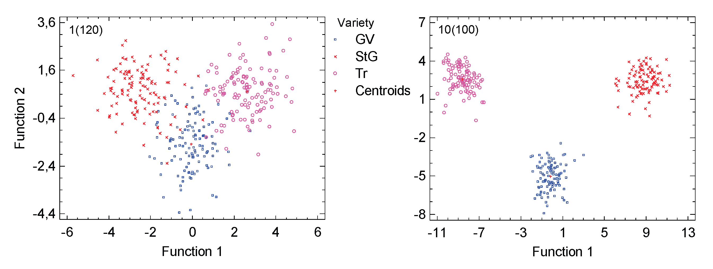
Figure 7.
Principal component analysis with composite leaves consisting of: all leaves of a variety; all leaves of a variety and a shoot position; all leaves of a variety, one year, and a shoot position. Each representation includes only composites of leaves from a position on the primary shoots: proximal (p) = shoot base, middle (m) = middle of the shoot, and distal (d) = near the shoot tip.
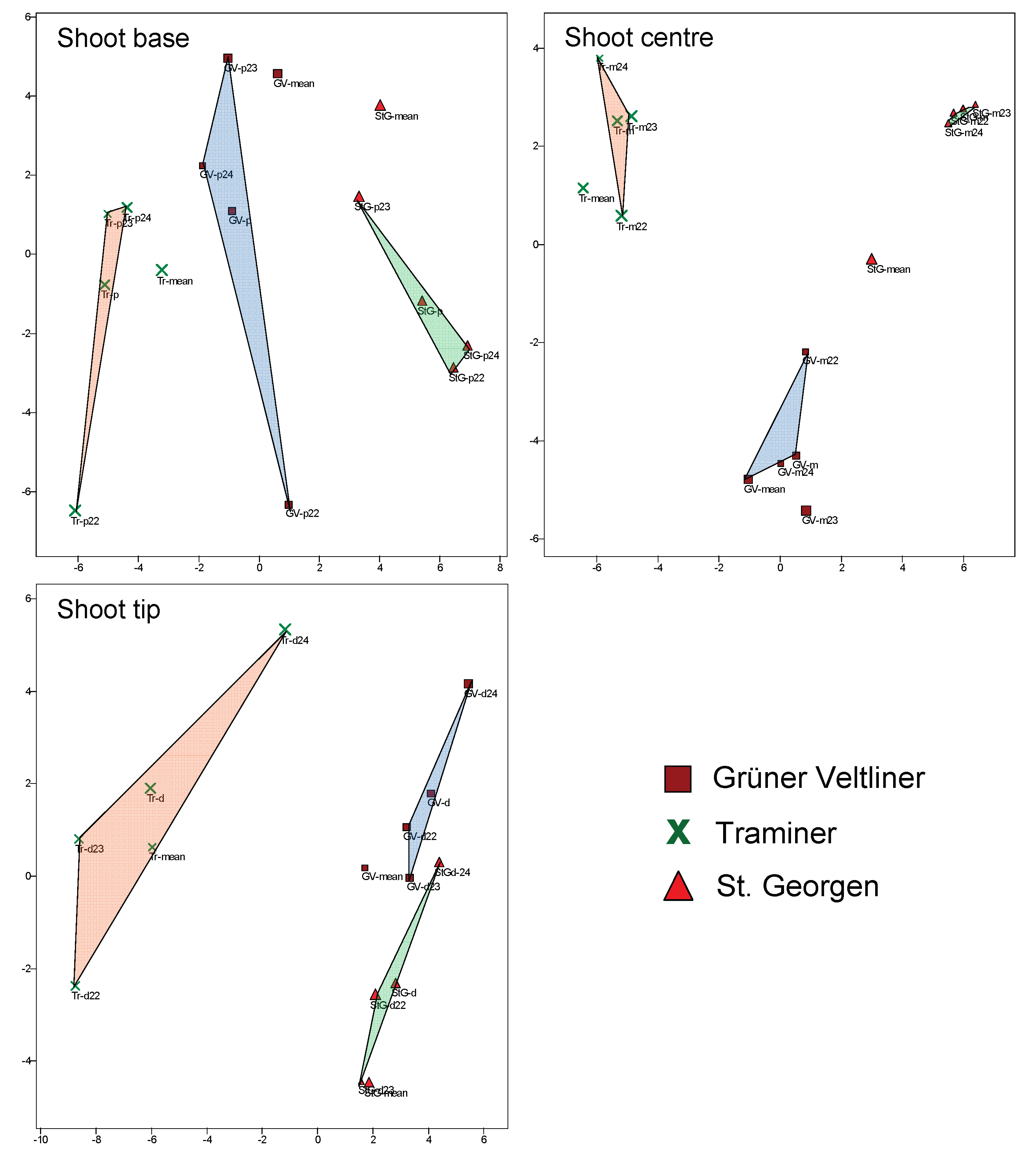
Figure 8.
PCA with composites consisting of all leaves from a seasonal time period, where on the left the collection season is divided into three equal intervals (DOY = Day of Year), and on the right into months. In each subfigure, there is also a composite for each variety that includes all the leaves (I-III and 4-10).
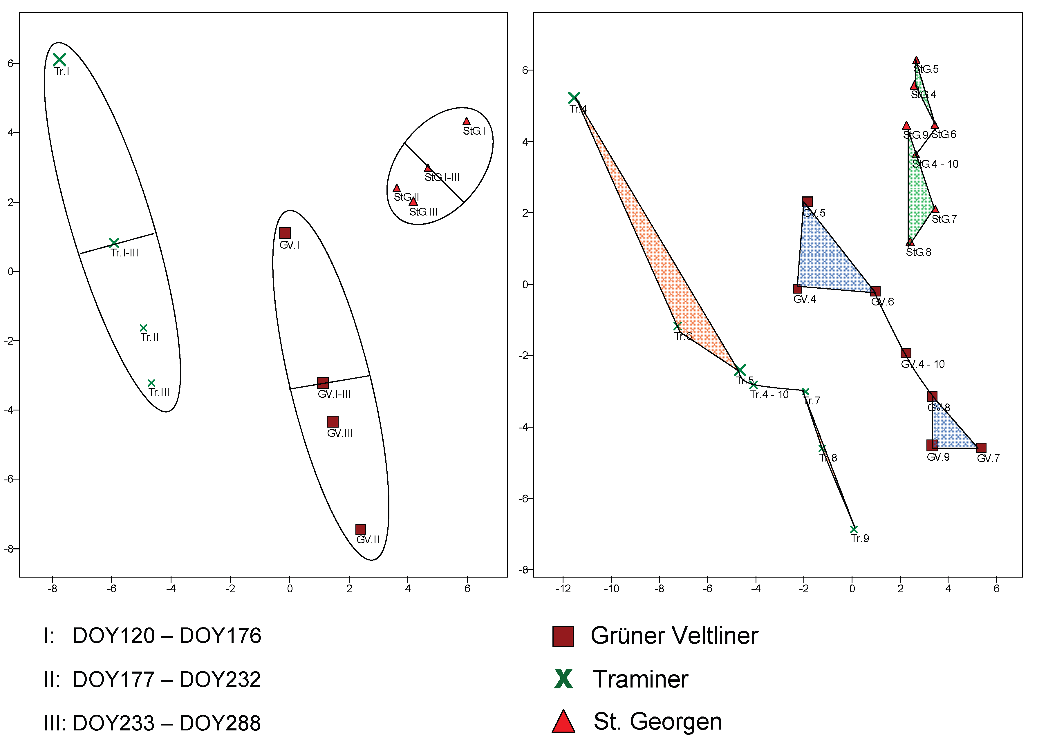
Figure 9.
More or less typical leaves for the three varieties are shown. However, individual variability is very high. Leaf areas that are typical for one variety and distinguish it from the other two are highlighted in color (see main text for more detailed explanations).
Figure 9.
More or less typical leaves for the three varieties are shown. However, individual variability is very high. Leaf areas that are typical for one variety and distinguish it from the other two are highlighted in color (see main text for more detailed explanations).
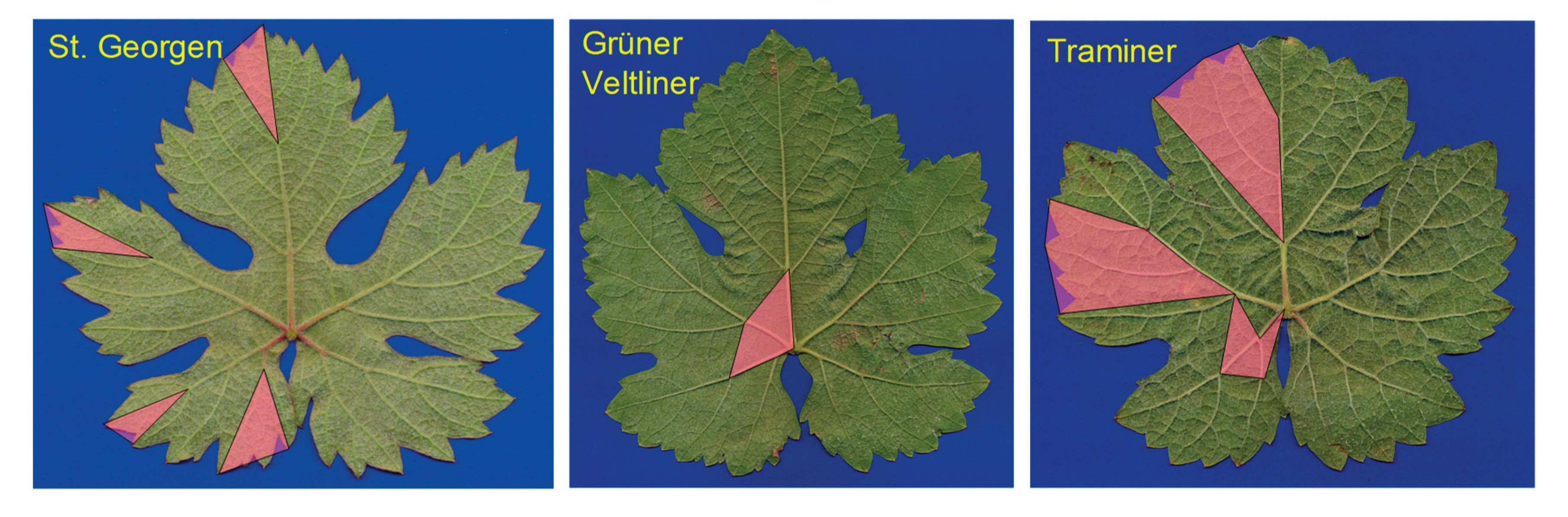
Figure 10.
Leaf length in comparison of the varieties and further differentiated by position on the shoot (Box-and-Whisker plot). GV: Grüner Veltliner; StG: St. Georgener-Rebe; Tr: Gewürztraminer; d: distal on the shoot; m: middle; p: proximal.
Figure 10.
Leaf length in comparison of the varieties and further differentiated by position on the shoot (Box-and-Whisker plot). GV: Grüner Veltliner; StG: St. Georgener-Rebe; Tr: Gewürztraminer; d: distal on the shoot; m: middle; p: proximal.

Figure 11.
Comparison of the relative area of the four leaf sectors for the varieties.
Disclaimer/Publisher’s Note: The statements, opinions and data contained in all publications are solely those of the individual author(s) and contributor(s) and not of MDPI and/or the editor(s). MDPI and/or the editor(s) disclaim responsibility for any injury to people or property resulting from any ideas, methods, instructions or products referred to in the content. |
© 2025 by the authors. Licensee MDPI, Basel, Switzerland. This article is an open access article distributed under the terms and conditions of the Creative Commons Attribution (CC BY) license (http://creativecommons.org/licenses/by/4.0/).
Copyright: This open access article is published under a Creative Commons CC BY 4.0 license, which permit the free download, distribution, and reuse, provided that the author and preprint are cited in any reuse.


