Submitted:
26 June 2025
Posted:
27 June 2025
You are already at the latest version
Abstract
Mathematical modeling plays a crucial role in supporting decision-making across a wide range of scientific disciplines. These models often involve multiple parameters, the estimation of which is critical to assessing their reliability and predictive power. Recent advancements in artificial intelligence have made it possible to efficiently estimate such parameters with high accuracy. In this study, we focus on modeling the dynamics of cryptocurrency market shares by employing a Lotka-Volterra system. We introduce a methodology based on a deep neural network (DNN) to estimate the parameters of the Lotka-Volterra model, which are subsequently used to numerically solve the system using a fourth-order Runge-Kutta method. The proposed approach, when applied to real-world market share data for Bitcoin, Ethereum, and alternative cryptocurrencies, demonstrates excellent alignment with empirical observations. Moreover, our method outperforms ARIMA models in terms of accuracy, showcasing its effectiveness for crypto market forecasting. The entire framework, including neural network training and Runge-Kutta integration, was implemented in MATLAB.
Keywords:
Lotka-Volterra
; Deep Neural Network
; MATLAB
; Runge-Kutta method
; Cryptocurrency
; Forecasting
1. Introduction
Over the past decade, blockchain technology has rapidly emerged as a transformative force, with many experts predicting it could reshape various aspects of modern society [1]. At its core, a blockchain is a decentralized, publicly accessible digital ledger [2]. While it is most commonly associated with cryptocurrencies-digital assets designed to function as a medium of exchange without the need for centralized oversight-it has far-reaching applications beyond that.Bitcoin, introduced in 2008 [2] under the pseudonym Satoshi Nakamoto (whose identity remains unknown and may represent either an individual or a group), stands as the pioneer and most widely recognized cryptocurrency. By December 2024, Bitcoin’s market capitalization soared to around 1.8 trillion euros [3], and it continues to maintain a strong market presence, currently valued above 1.4 trillion euros.The revolutionary concept introduced by Nakamoto not only sparked a dramatic surge in Bitcoin’s financial value but also inspired the creation of thousands of alternative cryptocurrencies. Today, over 17,000 digital currencies exist, either directly based on Bitcoin’s original blockchain or built on modified versions. This number continues to grow steadily. Beyond cryptocurrencies, blockchain technology has found applications across various sectors [4], with Decentralized Finance (DeFi) emerging as one of the most prominent.
A significant part of what has driven the success of cryptocurrencies is their strong focus on security and user privacy-features [5] that traditional financial systems often struggle to match. By utilizing advanced cryptographic protocols, digital currencies ensure the integrity of transactions and protect the anonymity of users. Additionally, the decentralized architecture behind most cryptocurrencies removes the need for central governing bodies [6], which not only reduces transaction costs but also improves efficiency and accessibility. Ethereum, one of the most prominent cryptocurrencies, has taken these innovations even further. It introduced smart contracts-self-executing agreements [6] coded directly onto the blockchain. These contracts automatically enforce their terms, offering greater transparency and eliminating the need for intermediaries. This breakthrough has significantly expanded the use cases for blockchain technology, pushing it beyond simple peer-to-peer payments into areas like decentralized finance (DeFi), gaming, and various Web3 applications.As of April 8, 2025, Ethereum’s market capitalization stands at approximately 167 billion euros [7]. This marks a significant decline compared to December 2024, when its market cap was valued at around 401 billion euros.The distinct benefits of blockchain-particularly its security, transparency, and decentralized control-continue to fuel the rise of cryptocurrencies like Ethereum. As the technology matures and adoption spreads, it’s likely to play an even more critical role in shaping the future of finance. Given Ethereum’s open-source nature, decentralized framework, and history of high returns, it has become a prime focus for investors and researchers alike, sparking growing interest in forecasting its price dynamics and understanding its long-term potential.
Cryptocurrencies have steadily gained prominence and are now playing an increasingly significant role in the global financial landscape. At their peak, the total market capitalization of digital assets approached 3 trillion euros, rivaling the valuations of some of the world’s largest publicly traded companies. What once began as an experimental domain for a niche group of tech-savvy enthusiasts has evolved into a mainstream asset class. The launch of Bitcoin futures in 2017 marked a turning point, and the approval of spot Bitcoin ETFs in January 2024 further solidified crypto’s presence in traditional financial markets. Initially driven by retail interest, the space has since attracted major institutional players [8], with many more expected to follow suit.
That said, the rise of crypto has not been without skepticism. Several traditional financial institutions remain wary, viewing cryptocurrencies as speculative bubbles rather than genuine innovations. Common criticisms include extreme price fluctuations, substantial energy demands, and relatively slow transaction speeds that hinder scalability and liquidity [9]. Some argue that neither Bitcoin nor blockchain has yet offered clear solutions to significant real-world problems.Nonetheless, regardless of whether these digital assets ultimately live up to their revolutionary promise, their current influence in the financial world is undeniable. As of today, the total market capitalization of all cryptocurrencies hovers around 3 trillion euros. A 2024 survey reported approximately 560 million active cryptocurrency users [10], highlighting the scale and reach of this emerging ecosystem.Unsurprisingly, the scientific community has taken a growing interest in cryptocurrencies, particularly through the lenses of complex systems and network theory. A considerable body of work has focused specifically on Bitcoin-examining its transactional network [11,12], price dynamics, and forecasting models [13,14]. However, only a limited number of studies have addressed the broader crypto market as a whole or attempted to model its complex behavior at the systemic level [15,16].
This study explores the behavior of cryptocurrency market shares by applying the Lotka-Volterra model to Bitcoin (BTC), Ethereum (ETH), and a combined group of alternative coins (ALTs). We compare BTC, ETH, and ALTs because they represent the three most significant and distinct segments of the cryptocurrency market. BTC (Bitcoin) is the original and dominant cryptocurrency, ETH (Ethereum) is the leading smart contract platform, and ALTs (altcoins) collectively capture all other cryptocurrencies, reflecting broader market trends and diversification. Given the dominance of a few major cryptocurrencies in total market capitalization, significant barriers to new entrants, and interdependent strategic behavior, the cryptocurrency market exhibits key characteristics of an oligopolistic structure. This justifies the application of competitive dynamics models, such as the Lotka-Volterra framework, to analyze the evolution of market shares and concentration . To determine the nonlinear interaction parameters within the system, we integrate a neural network trained on actual market data. This combined method effectively captures the competitive and cooperative dynamics between major digital assets. The estimated parameters from the neural network are then used to simulate the system’s evolution over time. Overall, the approach offers valuable insights into the structural behavior and shifts within the crypto market.The primary contribution of this study lies in analyzing the evolution of market structure and concentration by utilizing concepts from the evolutionary theory of population biology and population dynamics. Specifically, this research forecasts and models market evolution by employing the Lotka–Volterra framework, which is traditionally used to describe the competitive interactions between species vying for a shared, finite resource [17]. The primary objective of the proposed methodology is to offer an alternative approach for estimating the concentration level of a market with significant entry barriers, such as the cryptocurrency market. The Lotka–Volterra model utilized in this study has been applied successfully in various fields beyond biology, providing reliable estimates of the dynamics [18] within the processes it describes. Furthermore, the methodology proposed here can be integrated with existing frameworks or even used as a benchmark to validate their evaluation outcomes in the context of cryptocurrency markets.
Achieving the objectives outlined above would make significant contributions to both academic research and practical applications. It would offer novel approaches for estimating market concentration and provide an additional tool for strategic planning. When integrated with the recommendations presented in the conclusion, these efforts would lead to the creation of a comprehensive framework capable of capturing the various elements and factors that drive diffusion processes, particularly in the context of market competition and concentration levels.
2. Dynamics of Interacting Populations Under Competition
The hypothesis regarding population variation suggests that the rate of change is directly proportional to the current population size. The most widely accepted method for modeling species population growth in the absence of competition [19,20] is represented by the following equation:
Here, denotes the population size at time t, r represents the intrinsic growth rate, and K is the environmental carrying capacity-the maximum population the environment can sustain. This logistic model forms the basis of many demand estimation and forecasting techniques, including the logistic growth family [21] and Gompertz models [22].
When multiple species coexist in a shared ecosystem, they inevitably compete for limited resources. Definitions and explanations of such interspecies competition are found in [19] and [23], and can be summarized as follows: "Competition arises when two or more species experience diminished fitness-reduced growth or saturation levels-due to their simultaneous presence."
In such a scenario, each species’ access to resources diminishes due to the presence of others, resulting in decreased growth rates and reduced carrying capacities. More specific types of species [17] interaction have been categorized as:
- Predator-prey: One population’s growth decreases while the other’s increases.
- Competition: Growth rates of both populations decrease.
- Mutualism (symbiosis): Growth rates of both populations increase.
In the context of a closed and established cryptocurrency market, firms interact similarly: competition over limited market share can reduce the share of each participant, especially if they aim to maximize both market dominance and profits. This aligns with the second interaction type (competition), making it the most suitable analogy.
The simplest way to reflect this competition in a growth model is by introducing terms that quantify mutual interference. The resulting formulation is the Lotka–Volterra model, developed by Lotka and Volterra. This model has been thoroughly explored in the literature [17,20,23] for scenarios involving two or more interacting species.
For m competing participants (or entities) in a market [24,25], the system dynamics of Equation (1) can be described by the following set of first-order nonlinear differential equations:
In this expression, represents the rate of change of the i-th entity, is its individual growth coefficient, and measures the competitive effect of species j on species i (interspecies when , intraspecies when ). Note that these coefficients generally differ.
Each equation in this system can be derived by transforming the logistic growth equation as follows:
Additional terms are then included to represent the competitive interactions among entities in the market.
For the case where , the generalized Lotka–Volterra system described in Equation (2) is expressed as:
Here x,y, and z represent the three competing entities. The Lotka–Volterra formulation is particularly well-suited to capturing the nonlinear competitive dynamics among firms in a market. Its ability to incorporate interaction terms directly into the growth equations allows for more realistic modeling [26] of interdependencies, which are often nonlinear and time-varying. In contrast, traditional techniques such as linear regression are limited by their assumption of fixed relationships and fail to encapsulate these dynamic competitive effects. While agent-based models offer a more detailed view by simulating individual behaviors, they require significant computational power and detailed datasets, which may not always be feasible. Likewise, equilibrium-based models tend to ignore temporal changes, assuming static market conditions.
For these reasons, the Lotka–Volterra system stands out as a balanced and computationally efficient option that can both describe and predict the evolving nature of market competition. Similar modeling strategies have previously been applied to other sectors with promising results [27,28]. This system captures competition at a macro level and includes external influences-such as marketing variables-only implicitly. The key assumption is that such external factors remain constant throughout the study period. These factors may include global economic conditions (e.g., inflation, interest rates, recession fears), regulatory changes, investor sentiment, technological upgrades, and institutional adoption, all of which can significantly affect market dynamics. While these are not directly analyzed in this paper, their future incorporation would enable a more holistic model. In this paper, we develop a hybrid neural-network–Lotka–Volterra model as a generalized framework for forecasting cryptocurrency market dynamics and characterizing the competitive interactions and equilibrium among multiple assets. Future work will integrate exogenous drivers to capture both direct and indirect environmental influences.
3. Deep Neural Network Model for Crypto Dynamics
3.1. Feed Forward Neural Network Architecture
A feed forward neural network (NN) with three hidden layers as on Figure 1 was constructed to learn the temporal dynamics of the system. The architecture is described as follows:
- Input Layer: Accepts a single input feature corresponding to time, denoted as t.
- Hidden Layers: Three fully connected hidden layers, whith 10,6 and 9 neurons each and using the hyperbolic tangent (tanh) activation function. To promote stable learning, weights were initialized to small values and biases were set to zero.
- Output Layer: A fully connected layer with three outputs, representing the estimated values of the variables , , and . Each output is connected to a regression layer, which calculates the loss based on the deviation between predicted and actual values.
Function of the Neural Network:
- Time-Series Prediction: The neural network is trained on datasets to learn and predict their evolution over time. Once trained, it produces predictions for the three variables based solely on time input.
- Modeling Underlying Relationships: By learning from data, the NN approximates the hidden relationships between the variables and time, capturing complex and nonlinear behaviors that traditional models might overlook.
- Preparing for Optimization: After prediction, the outputs obtain continuous estimates of the state variables. These are then used to compute numerical derivatives , , and . These derivatives are essential for the next phase of analysis, where model parameters are estimated via optimization using lsqnonlin.
In essence, the neural network plays a crucial role in approximating the dynamics of the system, bridging the gap between observed data and the differential equations required for parameter identification.The neural network architecture with three hidden layers consisting of 10, 6, and 9 neurons respectively was selected based on bootstrap validation performance. Using moving block bootstrap resampling to simulate multiple training and testing scenarios, we compared several candidate architectures. The 10-6-9 configuration consistently achieved the lowest average test error and exhibited minimal performance variance across bootstrap samples, indicating strong generalization capability and robustness to data perturbations. The network’s depth allowed it to model nonlinear interactions among crypto market variables, while its compact structure minimized overfitting.
3.2. Feed-Forward Propagation
A feedforward neural network processes data points through a sequence of operations, as outlined in [29]. Given an input data point , the forward propagation begins by initializing the first layer activation as . To obtain the activations of layer l, denoted , from those of the previous layer , two main steps are followed.
First, an intermediate vector is calculated by multiplying the weight matrix with , then adding the corresponding bias vector :
This operation can be compactly written in matrix form as:
The second step applies the activation function element-wise to , producing the output activations :
Thus, for each input , both the pre-activation values and the activated outputs are computed using Equations (6) and (7). To highlight the dependence on the input sample , we can denote these layer-wise computations as . In matrix notation, the forward propagation for the entire dataset is summarized as:
This leads to a recursive formulation for the forward pass:
The final network output, represented by , is a function of the input and the learned parameters:
Alternatively, we may express the output in component form as:
where in (11) denotes the extraction of the j-th component from the final output vector .
4. Hybrid Neural Network–ODE Framework for Parameter Estimation and Forecasting
This section outlines the methodology developed for estimating parameters in dynamic systems governed by nonlinear ordinary differential equations (ODEs). Our approach utilizes a feedforward neural network in combination with optimization techniques to infer the unknown parameters. To demonstrate its practical utility, we apply the method to a Lotka-Volterra model describing the interactions among three major segments of the cryptocurrency market: Bitcoin, Ethereum, and altcoins. Time-series data for each segment is used, and the results highlight the model’s ability to accurately capture the system’s dynamic behavior.
Accurate parameter estimation in nonlinear dynamic systems is a key challenge across various domains, including financial forecasting. Traditional techniques often rely on simplifications such as linearization or require detailed prior knowledge of the system’s internal structure-assumptions that may not hold in complex financial ecosystems. In this work, we introduce a data-driven approach that leverages the flexibility of neural networks to model intricate dependencies, while employing numerical optimization to estimate the parameters of a nonlinear model. To provide clarity on the implementation, we also present the core steps of the algorithm used in our framework.
| Algorithm 1 Proposed Method |
|
4.1. Mathematical Formulation
As we see in the Algorithm 1 the neural network is trained to approximate the time evolution of the system by learning the mapping from time to the observed data [30]. After predicting the trajectories, we numerically compute the derivatives and fit them to a generalized Lotka–Volterra (GLV) model using nonlinear least squares optimization. The system of ODEs used to model the interactions among the three components (e.g., BTC, ETH, and ALTs) is given by:
To estimate the parameters , we define a residual function that quantifies the mismatch between the model’s predicted derivatives and the ones obtained from the neural network output. This residual function is given by:
In Equation (13) the derivatives are obtained from the neural network. Because the network is trained to output only, each time derivative must be computed by analytically differentiating the trained network with respect to t (using the chain rule through every hidden layer). Likewise, when forming for the lsqnonlin call, we should state explicitly that the input “” is this analytic network derivative rather than a numerical finite difference. The optimal parameters are obtained by minimizing the sum of squared residuals:
This optimization aligns the dynamics of the GLV model with the data-driven derivatives, effectively capturing the underlying interactions among the system components.
4.2. Numerical Integration via Runge–Kutta
Numerous numerical methods have been developed for solving ordinary differential equations. Among the most widely used for the integration of first- and second-order ODEs are the Runge-Kutta (-Nyström) schemes and linear multistep methods (e.g., see [31,32,33,34,35,36,37,38]).
The obtained coefficients are integrated into the Lotka-Volterra system (12) which is solved over the original time span using the classical 4th-order Runge-Kutta method [31]. The simulated trajectories are then compared to the observed data, and RMSE is computed to quantify fit quality.
The Runge-Kutta method approximates the solution to (15) through an iterative process defined by:
where
h represents the time step,
s denotes the number of stages in the method,
are the intermediate stage values,
are coefficients specifying the particular Runge-Kutta scheme.
From the general Runge-Kutta framework (16), various schemes of different algebraic orders can be derived. In this study, we utilize a fourth-order Runge-Kutta method with four stages [31].
Given an initial condition , the solution at the subsequent time step is calculated as:
For the classical RK4 method, the coefficients are:
This iterative procedure is applied at each time step, generating an approximate solution to the differential equation described by (15).
4.3. Model Evaluation
The neural network was trained using the Adam optimizer and epochs with initial learning rate were selected after experimenting with various values. To identify the optimal architecture, three different configurations of hidden layers were evaluated. In addition, multiple activation functions were tested, but the hyperbolic tangent (tanh) proved most effective, delivering the most stable and accurate results.
For performance evaluation, a moving block bootstrap validation approach was employed. This method resamples blocks of the original time series to generate multiple training and testing datasets, preserving temporal dependencies within each block. Unlike traditional cross-validation or walk-forward methods, bootstrap validation is particularly useful when dealing with limited data or non-stationary time series [39]. It allows for robust statistical inference and a more comprehensive understanding of the model’s generalization performance across different subsets of the data.We chose a block length of 10 time steps to span roughly one calendar month of share data, under the assumption that correlations persist over that window. We ran 5 bootstrap replicates, which we found sufficient to stabilize the out-of-bag (OOB) cost minima in preliminary tests. For each replicate, the OOB indices consist of all training points not selected by any block; the OOB cost is then computed on those held-out points to estimate generalization error. The replicate producing the lowest OOB cost is retained for the final neural-network weights. By applying this resampling technique, we obtained a realistic and statistically grounded estimate of the network’s prediction accuracy under data variability.
During training, a dynamic plot was used to monitor convergence and track loss reduction in real time. Once training was complete, the model was used to predict the time-dependent variables x(t), y(t), and z(t) across the full time horizon. The performance of the proposed method is highly influenced by both the choice of activation function and the strategy used for initializing weights and biases. The tanh function was chosen over sigmoid and ReLU because it centers outputs around zero, aiding in faster convergence and improving gradient propagation. Unlike sigmoid, tanh offers stronger gradients and mitigates the vanishing gradient issue, while also avoiding the “dead neuron” problem often associated with ReLU. Initial weights were drawn from a distribution of small values to keep the activation functions within their linear regions during early training, which promotes more stable learning dynamics. Similarly, initializing biases with small values prevents early saturation and preserves symmetry breaking across neurons. These combined practices contribute to improved stability, faster convergence, and higher accuracy, making the proposed framework well-suited for estimating parameters in complex nonlinear systems such as those modeling cryptocurrency market dynamics.
| Algorithm 2 Selection of Best Neural Network Architecture |
|
From Algorithm 2 we see that the DNN searched over all possible 3-hidden-layer DNN architectures (from 5 to 10 neurons per layer), for each learning rate and epoch combination.
From Table 1, we select the best architecture based on the mean RMSE.
RMSE evaluates the accuracy of predictions by measuring the average error between observed and predicted value, based on validation procedure:
Then, we extract the coefficients for all three and solve the system using the 4th-order Runge-Kutta method. Based on the comparison of the mean RMSE, we choose the best one, which we then include it in the graphs.
5. Numerical Experiment
5.1. Case Study Description
This study examines the historical market penetration and future prospects of the three crypto competitors.Monthly market share data for Bitcoin (BTC), Ethereum (ETH), and altcoins (ALTS) were sourced from CoinMarketCap historical snapshots [40], covering August 2015 to May 2023 as it is presented on Figure 2, a period of 93 months or almost 8 years.
The market share of alternative cryptocurrencies (ALTs) is derived by subtracting the shares of Bitcoin (BTC) and Ethereum (ETH) from 1, ensuring that the total market share across all segments sums to unity.
The initial step in assessing the performance of the proposed framework involves estimating the parameters of the Lotka-Volterra system defined in Equation (2) .While traditional approaches typically rely on predefined assumptions derived from the data, this study adopts a data-driven strategy. Specifically, a deep neural network is employed to infer the system parameters by effectively “training” the model based on time-series data of cryptocurrency market shares. This neural network-based estimation replaces heuristic techniques and enables the model to capture the underlying dynamics through optimization and learning from observed behavior. The results of the application of DNN for the case studied provided the following values for the corresponding parameters:
The estimated parameters, derived from neural network–assisted system identification, provide detailed insights into the mutual influences and self–regulatory mechanisms among Bitcoin (BTC, x), Ethereum (ETH, y), and Altcoins (ALTs, z) in the cryptocurrency market.
Intrinsic Growth Rates:
- (BTC), (ALTs), and (ETH) are all positive, indicating that each asset class would grow in isolation absent any competition or inhibition.
Intraspecies (Self-Interaction) Terms:
- (BTC) and (ETH) are negative, reflecting strong self-limitation (diminishing returns) as market share increases.
- (ALTs) is also negative, indicating that, unlike before, the Altcoin sector exhibits some self-inhibitory effects at high share levels.
Interspecies Interactions:
-
BTC Equation:
- –
- : A strong negative influence of ALTs on BTC, suggesting that as Altcoin share rises, BTC’s growth is sharply suppressed.
- –
- : A substantial positive effect from ETH on BTC, implying that Ethereum growth tends to bolster Bitcoin’s market share.
-
ETH Equation:
- –
- : A strong negative effect of BTC on ETH, reversing the previous supportive role—here Bitcoin dominance inhibits Ethereum.
- –
- : A very strong inhibitory influence of ALTs on ETH, indicating fierce competition from the broader Altcoin market.
-
ALT Equation:
- –
- : Bitcoin slightly inhibits Altcoins.
- –
- : Ethereum exerts a moderate negative effect on Altcoins.
- –
- : Confirms Altcoins also self-inhibit at high share.
Summary:
All three asset classes have positive intrinsic growth, but strong self-limitation and mutual inhibition dominate:
- BTC faces sharp suppression from Altcoins () and diminishing returns on its own share (). - ETH is heavily inhibited by both BTC () and ALTs (), despite its own positive growth rate. - ALTs, while intrinsically growing, experience self-inhibition () and competitive pressures from both BTC and ETH ().
These parameter signs suggest an intensely competitive market where no one asset can expand without encountering strong inhibitory forces from itself and its peers.
5.2. System Stability Testing
To investigate the local dynamics of the crypto market share model, we first estimate the parameters and from observed market data using a neural network combined with optimization techniques. These parameters define the nonlinear Lotka–Volterra system (12), where represent the market shares of BTC, ETH, and ALTs, respectively.
By setting the time derivatives to zero,
we solve the resulting algebraic system and find that it will eventually settle to an equilibrium of approximately for BTC, for ETH, and for ALTs:
This represents the steady-state market shares predicted by the model under the estimated parameters. To understand how the system behaves near this equilibrium, we linearize the nonlinear system (12) around . Denoting deviations from equilibrium as
the linearized dynamics satisfy
where is the Jacobian matrix of partial derivatives of the right-hand side of (12) evaluated at the equilibrium.
The general solution near equilibrium is
where and are the real eigenvalues and eigenvectors of , and the coefficients are obtained by projecting the initial deviation onto the eigenvector basis:
Analyzing the eigenvalues of , we find
all of which are strictly negative. This confirms that is a locally asymptotically stable node. The absence of any imaginary parts indicates purely monotonic convergence to equilibrium, without oscillatory transients.
The phase portrait shown in Figure 3 displays trajectories initiated from diverse market share configurations. All trajectories converge smoothly to the equilibrium , supporting the model’s predictive validity and its resilience to small perturbations.
This comprehensive approach—combining parameter estimation with Lotka–Volterra equilibrium analysis and linear stability theory—follows the methodology in [28], where the system’s long-term dynamics are characterized by a unique stable equilibrium. Hence, barring major external shocks, the model robustly predicts that cryptocurrency market shares will stabilize at .
5.3. Case Study Results
In this section, we compare the effectiveness of our hybrid DNN-RK4 method against a range of ARIMA models for predicting the market shares of BTC, ETH, and ALTs. The DNN-RK4 approach demonstrates the closest alignment to the real-world market share data, consistently producing the lowest prediction errors across the tested period.
The ARIMA (AutoRegressive Integrated Moving Average) model is a widely used statistical method for analyzing and forecasting time-series data. It combines three components: the autoregressive (AR) part models the relationship between current and past values; the integrated (I) part handles non-stationarity by differencing the data; and the moving average (MA) part captures dependencies between residual errors. By adjusting its parameters (p, d, q), ARIMA can effectively model and forecast trends and patterns in sequential financial data, including cryptocurrency prices. In the ARIMA model, p denotes the order of the autoregressive component (i.e., the number of lagged values of the series included), d represents the degree of differencing applied to make the series stationary (i.e., the number of times the series is replaced by the difference between consecutive observations), and q specifies the order of the moving-average component (i.e., the number of lagged forecast errors incorporated). Together, these three parameters allow ARIMA models to capture both short-term autocorrelation (through p and q) and nonstationarity (through d) in time series data.
The various ARIMA configurations [42], while capable of capturing some of the underlying temporal patterns, generally yield higher Root Mean Squared Error (RMSE) values compared to the DNN-RK4 method. To facilitate an objective assessment, all models are evaluated using the RMSE metric, and results are summarized both in graphical form and in a results table.
This analysis provides strong evidence that the DNN-RK4 method offers superior predictive power for modeling the evolution of cryptocurrency market shares when compared to traditional ARIMA time series approaches.
To evaluate the forecasting accuracy of the proposed DNN-RK4 approach, grounded in a nonlinear dynamical system framework, we compared its performance with that of classical time series models, specifically ARIMA. We evaluated multiple ARIMA configurations, including , , and . For each candidate model, we fitted the parameters on the training set and computed the RMSE on the validation set. The ARIMA configuration produced the lowest RMSE, and was therefore chosen for comparison against our proposed method. The comparison focuses on the three main components of the market: Bitcoin (BTC), Ethereum (ETH), and alternative cryptocurrencies (ALTs).
The DNN-RK4 model, driven by parameters estimated through a neural network, exhibited superior predictive performance across all market segments. For BTC, the RK4 model achieved an RMSE of 0.06865, significantly outperforming the ARIMA model’s RMSE of 0.14742 as we notice on Figure 4. In the case of ETH, we see on Figure 5 that the differential was similarly notable-0.02682 (RK4) compared to 0.03665 (ARIMA). For the ALT category, the DNN-RK4 model again showed improved accuracy, reducing the error from 0.11890 (ARIMA) to 0.05581 as shown in Figure 6. These results highlight the advantage of using a model based on competitive dynamics to capture nonlinear relationships inherent in the cryptocurrency ecosystem, where investor behavior, technological updates, and market sentiment evolve rapidly.
The cryptocurrency market is characterized by high volatility, interdependence between major assets, and continuous entry of new tokens. These features make traditional linear models less effective in capturing complex feedback mechanisms and competitive interactions. The DNN-RK4 method, supported by neural network-driven parameter learning, demonstrates strong adaptability in forecasting such nonlinear systems. It is particularly useful in capturing turning points and saturation effects, which are common in speculative and innovation-driven markets like crypto.
Further supporting these observations, Table 2 compares RMSE values across multiple modeling strategies. The DNN-RK4 model, in particular, demonstrated excellent forecasting capabilities, with RMSE values of 0.06865, 0.02682, and 0.05581 for BTC, ETH, and ALTs, respectively. Compared to more traditional techniques-including ARIMA model approaches-the DNN-RK4 consistently provided more accurate results, affirming its effectiveness in modeling the dynamic interactions of market share evolution in a decentralized digital asset environment.
6. Discussion
To further improve the robustness and accuracy of cryptocurrency market modeling, future research will investigate a range of advanced machine learning and hybrid approaches tailored to the unique challenges of crypto dynamics. One promising direction involves Temporal Convolutional Networks (TCNs) [43], which can outperform recurrent models in sequence modeling tasks while offering parallel processing advantages and stable gradients over long sequences-a critical factor when analyzing extensive crypto market histories.
In addition, the use of Graph Neural Networks (GNNs) will be explored to represent the complex interdependencies between different cryptocurrencies [44]. Crypto assets often exhibit co-movements, influenced by trading volumes, blockchain correlations, or investor sentiment. Modeling these relationships as a graph enables more informed parameter estimation and can uncover hidden structures in the market.
Another area of potential is Neural ODEs, which integrate the strengths of neural networks with differential equations. This approach is particularly suitable for learning continuous-time representations, offering a natural fit for systems like Lotka–Volterra that evolve over time. Neural ODEs can adaptively model temporal changes in market competition and volatility with fewer parameters and better interpretability [45].
The integration of Sentiment Analysis from social media and blockchain news will also be considered. Since investor behavior in crypto is highly reactive to news, incorporating textual data through models like BERT or domain-specific transformer variants (e.g., FinBERT) could improve forecasting accuracy by providing context-aware inputs to dynamic models [46].Finally, online learning techniques will be examined for their ability to continuously update model parameters as new data arrives. This is critical for maintaining prediction accuracy in a market characterized by rapid innovation, regulatory shifts, and speculative bubbles. Something important to note here is that, because our Lotka–Volterra model assumes constant coefficients, it cannot capture one-time shocks such as Bitcoin’s May 2020 halving or regulatory crackdowns in 2021. As a result, the estimated parameters may partially reflect these exogenous events rather than pure “peer competition.” Future work will incorporate time-varying coefficients, exogenous covariates, and the previously discussed methodologies to address this limitation, aiming to develop a more comprehensive, adaptive, and robust framework for modeling and forecasting market share evolution in the cryptocurrency domain.
7. Conclusions
The proposed framework demonstrates that integrating deep neural networks with Lotka–Volterra competitive dynamics provides a robust, data-driven means of capturing and forecasting the evolving structure of cryptocurrency market shares. By estimating interaction coefficients directly from observed BTC, ETH, and ALT time series and then simulating their joint evolution via a fourth-order Runge–Kutta scheme, the model not only outperforms traditional ARIMA benchmarks but also yields interpretable insights into mutual competitive pressures (e.g., the asymmetric influence of BTC on ALTs and ETH on BTC). Moreover, local stability analysis confirms that the estimated equilibrium remains locally asymptotically stable, explaining why any transient deviations decay in the absence of exogenous shocks.These findings both validate the Lotka–Volterra–NN hybrid approach in a highly nonlinear, volatile domain and furnish a principled basis for strategic decision-making. Looking ahead, extending the model to accommodate time-varying coefficients, exogenous covariates, or graph-based interactions among a broader set of tokens could further enhance its adaptability and predictive power, ensuring that it remains responsive to the rapid innovation and intermittent shocks characteristic of global crypto markets.
Author Contributions
D.K., D.P. and K.G. conceived of the idea, designed and performed the experiments, analyzed the results, drafted the initial manuscript and revised the final manuscript. All authors have read and agreed to the published version of the manuscript.
Funding
This research was supported by Grant (81845) from the Research Committee of the University of Patras via “C. CARATHEODORI” program.
Institutional Review Board Statement
Not applicable.
Informed Consent Statement
Not applicable.
Data Availability Statement
The raw data used in this study are publicly available online at https://coinmarketcap.com/historical/. The specific dataset used for analysis is also provided in the supplementary material.
Conflicts of Interest
The authors declare no conflicts of interest.
References
- White GRT. Future applications of blockchain in business and management: A Delphi study . Strategic Change ,2017, 26, 439–451. [CrossRef]
- Bitcoin.org. Available online: https://bitcoin.org/bitcoin.pdf.
- Tradingview.com. Available online: https://www.tradingview.com/symbols/BTC/.
- Taleb, N. et al.Prospective applications of blockchain and bitcoin cryptocurrency technology . TEM J ,2019, 8, 48–55. [CrossRef]
- Navamani, T. M. A Review on Cryptocurrencies Security . Journal of Applied Security Research ,2021, 18(1), 49–69. [CrossRef]
- T. Nandy, U. Verma, P. Srivastava, D. Rongara, A. Gupta and B. Sharma.The Evaluation of Cryptocurrency: Overview, Opportunities, and Future Directions . 2023 7th International Conference on Intelligent Computing and Control Systems (ICICCS) ,2023, 1421–1426. [CrossRef]
- Tradingview.com. Available online: https://www.tradingview.com/symbols/ETH/.
- Forbes.com. Available online: https://www.forbes.com/sites/lawrencewintermeyer/2021/08/12/institutional-money-is-pouring-into-the-crypto-market-and-its-only-going-to-grow/?sh=1a5424261459.
- Nicholas Taleb, N.Bitcoin, currencies, and fragility . Quantitative Finance ,2021, 21(8), 1249–1255. [CrossRef]
- VISUAL CAPITALIST. Available online: https://www.visualcapitalist.com/crypto-ownership-growth-by-region/.
- Javarone, M. A. and Wright, C. S.From bitcoin to bitcoin cash: A network analysis . In Proceedings of the 1st Workshop on Cryptocurrencies and Blockchains for Distributed Systems ,2018, 77–81. [CrossRef]
- Donet, J. A. D., Pérez-Sola, C. and Herrera-Joancomartí, J.The bitcoin p2p network . In International conference on financial cryptography and data security ,2014, 87–102. [CrossRef]
- Kjærland, F., Khazal, A., Krogstad, E. A., Nordstrøm, F. B. and Oust. An analysis of bitcoin’s price dynamics . J. Risk Financ. Manag ,2018,11, 63. [CrossRef]
- Velankar, S., Valecha, S. and Maji, S.Bitcoin price prediction using machine learning . In 2018 20th International Conference on Advanced Communication Technology (ICACT) ,2018, 144–147.
- ElBahrawy Abeer, Alessandretti Laura, Kandler Anne, Pastor-Satorras Romualdo and Baronchelli Andrea.2017Evolutionary dynamics of the cryptocurrency markeT . R. Soc. Open Sci ,2017, 4:170623. [CrossRef]
- Wu, K., Wheatley, S. and Sornette .Classification of cryptocurrency coins and tokens by the dynamics of their market capitalizations . Soc. Open Sci ,2018, 5, 180381. [CrossRef]
- J.D. Murray.Mathematical Biology. Springer-Verlag, ,1993, New York.
- A. W. Wijeratnea, F. Yi, and J. Wei. “Biffurcation analysis in the diffu- sive Lotka-Voltera system: An application to market economy. Chaos,Solitons Fractals, ,2009, vol. 40 , 902–911. [CrossRef]
- D. Neal.Introduction to Population Biology. New York: Cambridge University Press, ,2004.
- W. E. Boyce and R. C. DiPrima .Elementary Differential Equations and Boundary Value Problems, . Hoboken, NJ: Wiley, ,2004, 8th ed.
- J. C. Fisher and R. H. Pry .“A simple substitution model of technological change,” . Technol. Forecast. Soc. Change, ,1971, vol. 3, 75–88. [CrossRef]
- L. P. Rai.“Appropriate models for technology substitution” . J. Sci. Ind. Res. ,1999, vol. 58 , 14–18.
- M. Begon, C. Townsend, and J. Harper. Ecology: From Individuals to Ecosystems . Oxford, U.K.: Blackwell ,2006, 4th ed.
- T. H. Fay and J. C. Greeff. “A three species competition model as a decision support tool” . Ecol. Modell ,2008, vol. 211,, 142–152. [CrossRef]
- P. G. L. Leach and J. Miritzis.“Analytic behaviour of competition among three species” . J. Nonlinear Math. Phys ,2006, vol. 13, 535–548. [CrossRef]
- Olivença DV, Davis JD and Voit EO. Inference of dynamic interaction networks: A comparison between Lotka-Volterra and multivariate autoregressive models . Front. Bioinform ,2022, Volume 2. [CrossRef]
- Kastoris, D.; Giotopoulos, K.; Papadopoulos, D. Neural Network-Based Parameter Estimation in Dynamical Systems . Information ,2024, vol. 15, 809. [CrossRef]
- C. Michalakelis, T.S. Sphicopoulos, D. Varoutas.Modelling competition in the telecommunications market based on the concepts of population biology.Transactions on Systems, Man and Cybernetics. Part C: Applications and Reviews 4 2011, 200–210. [CrossRef]
- G. Bebis and M. Georgiopoulos. Feed-forward neural networks . In IEEE Potentials ,1994, Vol 13 (4), 27–31.
- L. Huang, J. Qin, Y. Zhou, F. Zhu, L. Liu and L. Shao. Normalization Techniques in Training DNNs: Methodology, Analysis and Application . in IEEE Transactions on Pattern Analysis and Machine Intelligence ,2023, vol. 45, no. 8, 10173-10196. [CrossRef]
- J. C. Butcher.Numerical Methods for Ordinary Differential Equations . 3 ,2016, 10, 143–331. [CrossRef]
- Tan Delin , Chen Zheng. "On A General Formula of Fourth Order Runge-Kutta Method" . Journal of Mathematical Science & Mathematics Education, ,2012, 7(2), 1–10.
- J. R. Dormand, M. E. A. El-Mikkawy, P. J. Prince.Families of Runge-Kutta-Nyström formulae . IMA J. Numer ,1987, 7, 235–250. [CrossRef]
- D. F. Papadopoulos, T. E. Simos.A new methodology for the construction of optimized Runge-Kutta- Nyström methods . International Journal of Modern Physics C ,2011, 22 (6), 623–634. [CrossRef]
- D. F. Papadopoulos, T. E. Simos. The use of phase lag and amplification error derivatives for the construction of a modified Runge-Kutta-Nyström method. Abstract and Applied Analysis ,2013, 910624. [CrossRef]
- Papadopoulos, D.F., Anastassi, Z.A., Simos, D.F. The use of phase-lag and amplification error derivatives in the numerical integration of ODEs with oscillating solutions. AIP Conference Proceedings , 2009. [CrossRef]
- Papadopoulos, D.F., Anastassi, Z.A., Simos, D.F. A zero dispersion RKN method for the numerical integration of initial value problems with oscillating solutions. AIP Conference Proceedings , 2009. [CrossRef]
- Papadopoulos, D.F. A Parametric Six-Step Method for Second-Order IVPs with Oscillating Solutions. Mathematics ,2024, vol. 12, 3824. [CrossRef]
- Steyerberg, Ewout W,Harrell, Frank E, Jr ,Borsboom, Gerard J.J.M,Eijkemans, M.J.C,Vergouwe, Yvonne,Habbema, J.Dik F.Internal validation of predictive models: Efficiency of some procedures for logistic regression analysis . Journal of Clinical Epidemiology ,2001, 54 (8), 774–781. [CrossRef]
- coinmarketcap.com. Available online: https://coinmarketcap.com/historical/.
- Schulz, A. W. Equilibrium modeling in economics: a design-based defense. Journal of Economic Methodology ,2024, 31(1), 36–53. [CrossRef]
- Kontopoulou, V.I.; Panagopoulos, A.D.; Kakkos, I.; Matsopoulos, G.K. A Review of ARIMA vs. Machine Learning Approaches for Time Series Forecasting in Data Driven Networks . Future Internet ,2023, 15, 255. [CrossRef]
- Ying Liu, Xiaohua Huang, Liwei Xiong, Ruyu Chang, Wenjing Wang, Long Chen. Stock price prediction with attentive temporal convolution-based generative adversarial network . Array ,2025, 25. [CrossRef]
- Zening Zhao, Jinsong Wang, Jiajia Wei. Graph-Neural-Network-Based Transaction Link Prediction Method for Public Blockchain in Heterogeneous Information Networks . Blockchain: Research and Applications ,2025. [CrossRef]
- Coelho, C.; da Costa, M.F.P.; Ferrás, L.L. XNODE: A XAI Suite to Understand Neural Ordinary Differential Equations . AI ,2025, 6, 105. [CrossRef]
- Vincent Gurgul, Stefan Lessmann, Wolfgang Karl Härdle. Deep learning and NLP in cryptocurrency forecasting: Integrating financial, blockchain, and social media data . International Journal of Forecasting ,2025. [CrossRef]
Figure 1.
An example of a deep neural network with one input neuron, three output neurons and three hidden layers, with 10,6 and 9 neurons.
Figure 1.
An example of a deep neural network with one input neuron, three output neurons and three hidden layers, with 10,6 and 9 neurons.
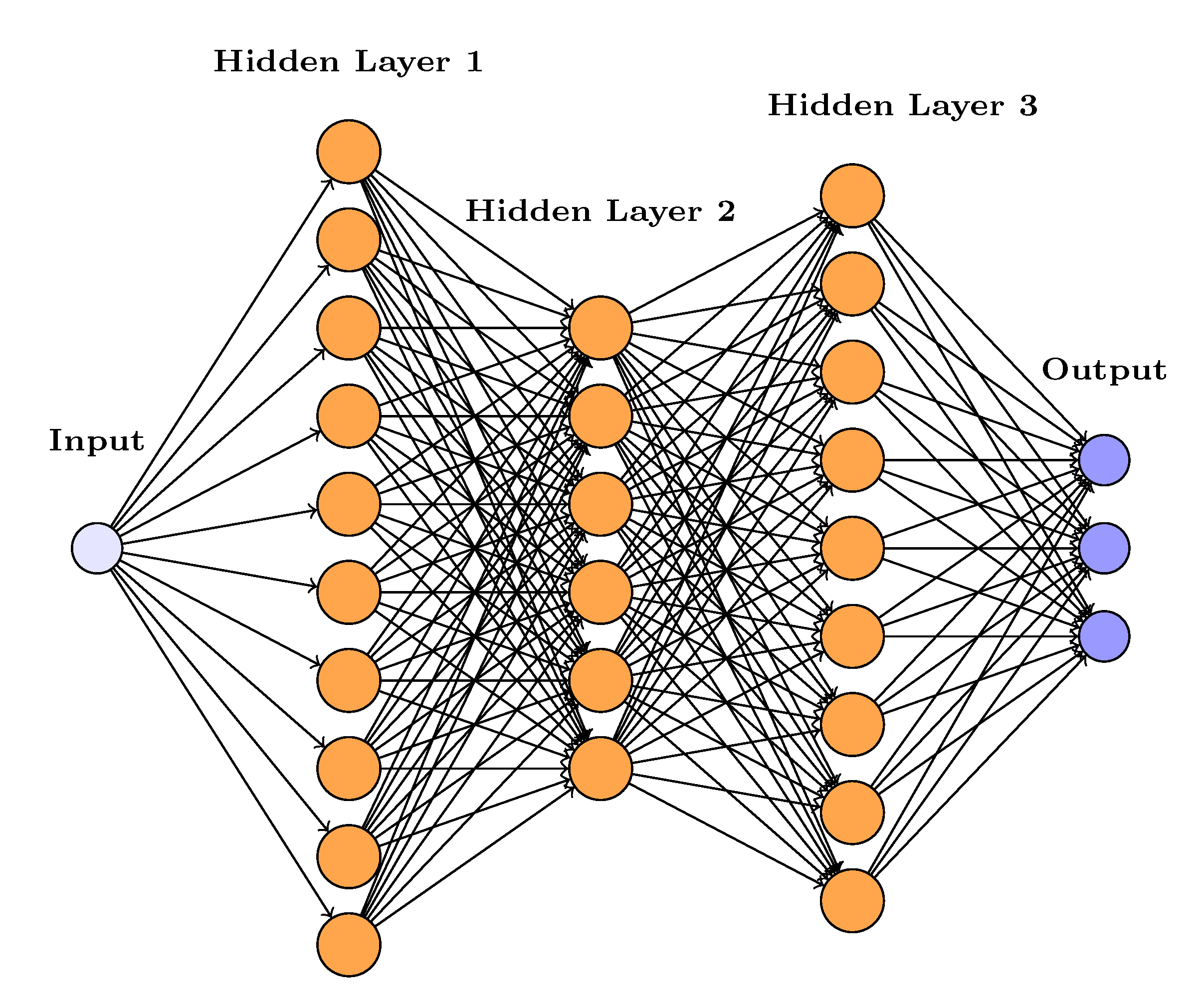
Figure 2.
Evolution of cryptocurrency market from August 2015 to May 2023.
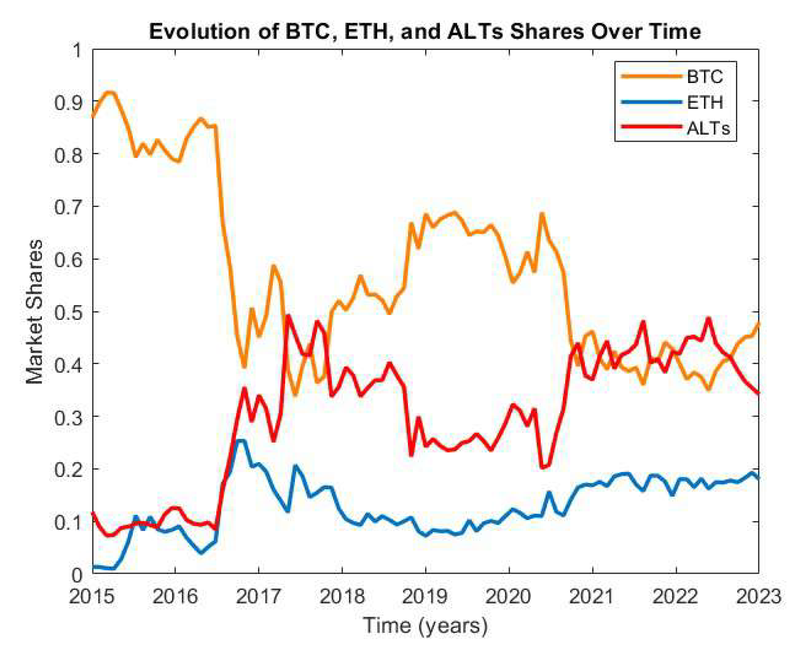
Figure 3.
Trajectories from various initial market shares converging to the unique stable equilibrium .
Figure 3.
Trajectories from various initial market shares converging to the unique stable equilibrium .
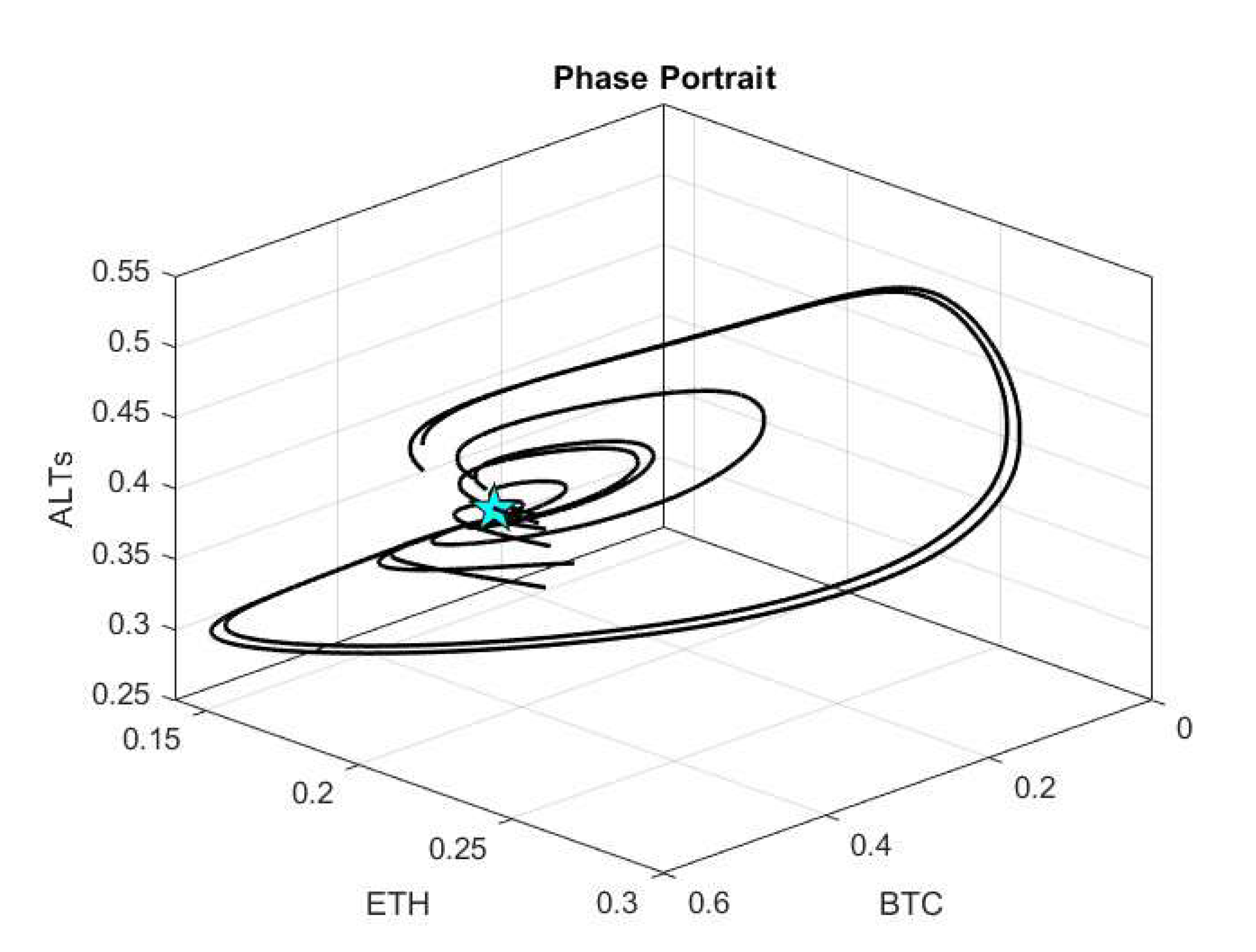
Figure 4.
Comparison of BTC.
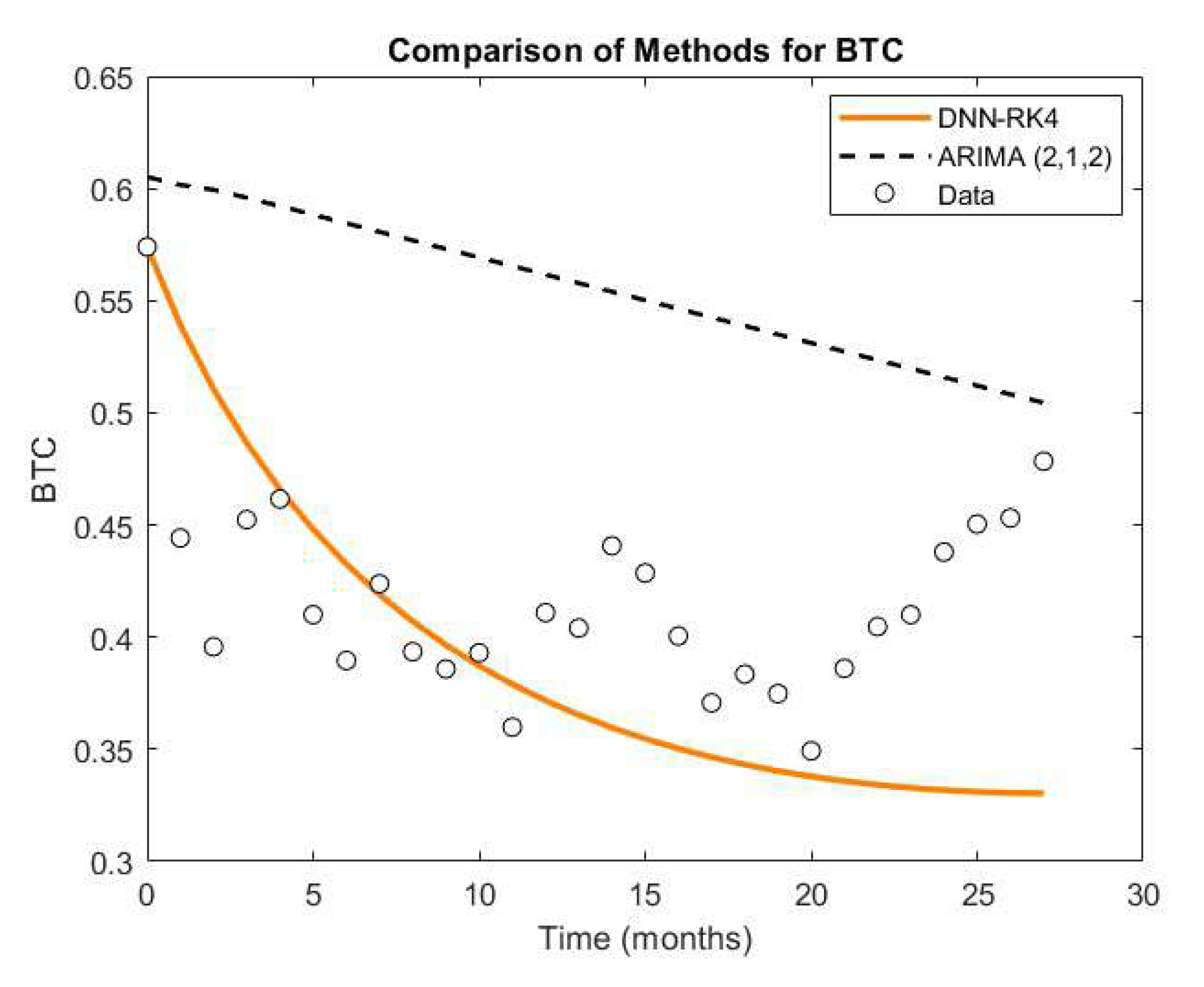
Figure 5.
Comparison of ETH.
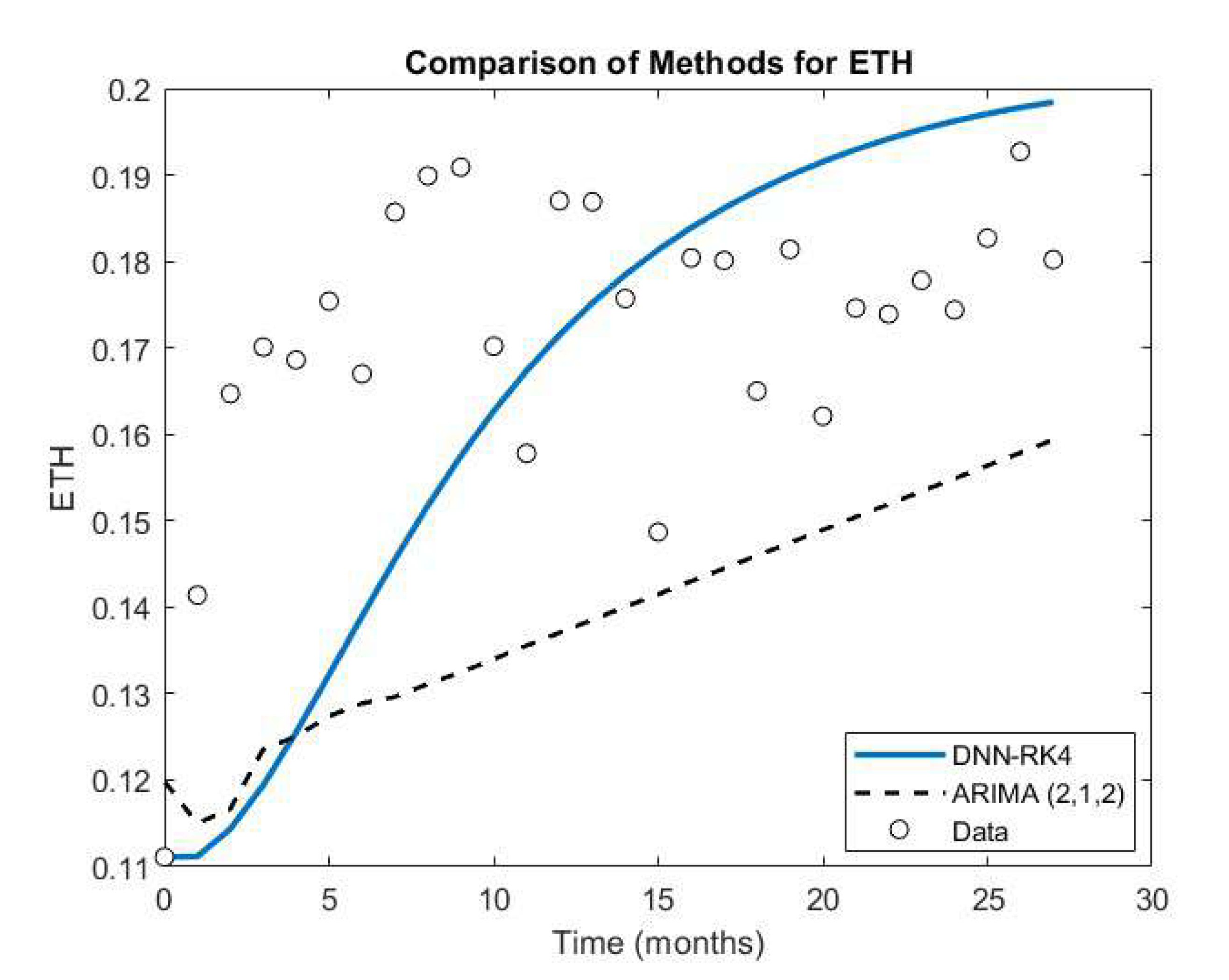
Figure 6.
Comparison of ALTs.
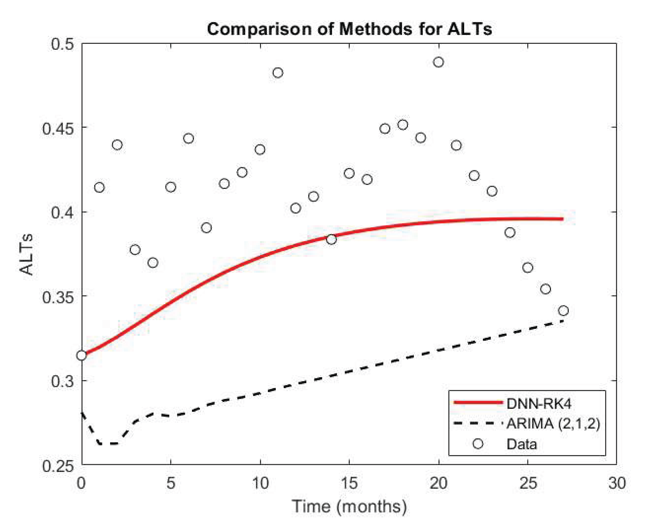

Table 1.
Per-asset RMSEs (BTC, ETH, ALTs) and mean RMSE (MRMSE) for various NN architectures and hyperparameters.
Table 1.
Per-asset RMSEs (BTC, ETH, ALTs) and mean RMSE (MRMSE) for various NN architectures and hyperparameters.
| BTC | ETH | ALTs | MRMSE | LR | Epochs | |||
| 10 | 6 | 9 | 0.056355 | 0.097497 | 0.096556 | 0.083469 | 0.0001 | 200 |
| 10 | 6 | 9 | 0.063268 | 0.092336 | 0.097758 | 0.084454 | 0.0001 | 100 |
| 8 | 10 | 10 | 0.068767 | 0.097675 | 0.101360 | 0.089267 | 0.0001 | 200 |
| 7 | 7 | 6 | 0.062612 | 0.100960 | 0.102480 | 0.088684 | 0.0001 | 200 |
| 7 | 10 | 10 | 0.071430 | 0.096462 | 0.102860 | 0.090251 | 0.0001 | 200 |
| 6 | 5 | 10 | 0.063437 | 0.101870 | 0.102940 | 0.089416 | 0.0001 | 200 |
| 9 | 10 | 5 | 0.071015 | 0.099051 | 0.103100 | 0.091055 | 0.00005 | 200 |
| 9 | 9 | 10 | 0.068600 | 0.099730 | 0.104540 | 0.090957 | 0.0001 | 200 |
| 10 | 8 | 10 | 0.058409 | 0.114040 | 0.105150 | 0.092533 | 0.0001 | 200 |
| 9 | 10 | 5 | 0.072399 | 0.100790 | 0.105270 | 0.092820 | 0.0001 | 100 |
Table 2.
Root Mean Squared Error (RMSE) values for different methods and components BTC, ETH and ALTs.
Table 2.
Root Mean Squared Error (RMSE) values for different methods and components BTC, ETH and ALTs.
| Method | RMSE for BTC | RMSE for ETH | RMSE for ALTs |
|---|---|---|---|
| DNN-RK4 | 0.06865 | 0.02682 | 0.05581 |
| ARIMA (2,1,2) | 0.14742 | 0.03665 | 0.11890 |
Disclaimer/Publisher’s Note: The statements, opinions and data contained in all publications are solely those of the individual author(s) and contributor(s) and not of MDPI and/or the editor(s). MDPI and/or the editor(s) disclaim responsibility for any injury to people or property resulting from any ideas, methods, instructions or products referred to in the content. |
© 2025 by the authors. Licensee MDPI, Basel, Switzerland. This article is an open access article distributed under the terms and conditions of the Creative Commons Attribution (CC BY) license (http://creativecommons.org/licenses/by/4.0/).
Copyright: This open access article is published under a Creative Commons CC BY 4.0 license, which permit the free download, distribution, and reuse, provided that the author and preprint are cited in any reuse.


