Submitted:
25 June 2025
Posted:
26 June 2025
You are already at the latest version
Abstract
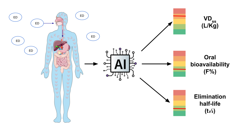
Toxicokinetics (TK) properties are essential in the framework of chemical risk assessment and drug discovery. Indeed, a TK profile provides information about the fate of chemicals in the human body. In this context, Quantitative Structure-Activity Relationship (QSAR) models are convenient computational tools to predict TK properties. Here, we developed QSAR models for the prediction of two TK properties: oral bioavailability and volume of distribution at steady state (VDss). We collected and curated two large sets of 1712 and 1591 chemicals for respectively oral bioavailability and VDss and compared regression and classification (binary and multiclass) models with the application of several machine learning algorithms. The best predictive performance of the models for regression (R) prediction is characterized by a Q²F3 equal to 0.34 with the R-CatBoost model, for oral bioavailability, and a Geometric Mean Fold Error (GMFE) equal to 2.35 for VDss with the R-RF model. The models were then applied on a list of potential endocrine disrupting chemicals (EDC), highlighting chemicals with a high probability of posing a concern on human health due to their TK profile. Based on the results obtained, insights about structural determinants of TK properties for EDCs are also further discussed.
Keywords:
QSAR
; oral bioavailability
; volume of distribution
; endocrine disrupting chemicals
; toxicokinetics
1. Introduction
Pharmacokinetics (PK) in the realm of drugs refer to the characterization of absorption, distribution metabolism, and excretion of xenobiotics in the organism [1]. Toxicokinetics (TK) is closely related to pharmacokinetics (PK), as it involves the generation of PK data either as part of nonclinical toxicity studies or through dedicated supportive studies to evaluate systemic exposure. Such analyses are largely used in pharmaceutical and chemical industries as they are critical for gaining insights into TK propensities of potential drug candidates and for the assessment of risk associated with environmental chemicals [2,3].
To limit the cost of such experiments and still provide relevant information for decision-makers in the field of drug discovery and chemical risk assessment, in silico models capable of predicting keys TK/PK properties, notably oral bioavailability and volume of distribution (VD) are commonly developed as a first estimation [4].
Oral bioavailability characterizes the fraction of an orally administered drug that reaches the systemic circulation (F%). It is calculated considering the relationship between plasma chemical concentration vs. time after administration. Oral bioavailability is defined as the percentage of the dose area under the curve of the concentration of chemicals in the plasma after oral administration divided by the dose area under the curve of the concentration of drugs in the plasma after intravenous administration [5]. This comparison informs about the proportion of chemicals reaching the bloodstream since intravenous administration avoids the digestive system and first-pass metabolism. A high oral bioavailability value can result in exposure of toxic compounds after intake and low oral bioavailability for drugs can result in an increase in the dose needed with associated risk of toxicity through accumulation and metabolites [6].
The volume of distribution (VD) measures the ability of a chemical to remain in plasma or to redistribute to other tissue compartments. VD is computed by considering the amount of a chemical in the body divided by the plasma concentration of the same chemical [7]. In the field of drug discovery, having a priori knowledge about VD assists in optimizing drug therapies, avoiding undesirable effects, while proposing effective treatments. Indeed, at a constant clearance, a chemical with high VD will have a longer elimination half-life than a chemical with low VD [8], since a chemical will persist in tissues while being slowly released in the bloodstream. Therefore, knowing the VD of environmental chemicals is also important in the field of chemical risk assessment since, these chemicals might remain longer in tissue which could lead to accumulation in the human body and so resulting in toxicity, especially for lipophilic drugs [6]. There are different types of VD terms commonly used with the volume of distribution at steady state (VDss) is generally the most relevant as it is used to determine VD associated with the steady-state dosing of the chemical. It is calculated during the phase called “steady state” when the distribution and elimination phase are equal [7].
Several computational studies have been developed to predict oral bioavailability [9,10,11,12,13,14,15,16] and VDss, notably QSAR models [17,18,19,20,21]. Most existing models have focused on oral bioavailability using classification approaches, while regression models have been primarily developed for VDss , using notably the Lombardo et al. dataset [17]. In our work, we combined datasets from multiple sources, including a newly developed dataset from Liu et al. [22].
In this context, we decided to collect a large dataset of chemicals and to develop different modeling algorithms for regression, binary- and multi-class prediction for oral bioavailability and VDss.
The more relevant models were then used to assess the TK properties of potential endocrine disrupting chemicals (EDC). The focus on this category of chemicals has been motivated by the fact that EDC can disrupt the endocrine system and cause cancer, metabolic disorders, neurocognitive functions, infertility, immune diseases, and allergies [23,24,25,26,27] through an interference with the estrogen, androgen, and thyroid hormone receptors, steroidogenesis (ER, AR, and TR)-mediated effects [28]. So, predicting potential EDC with a high oral bioavailability and high VDss could be relevant for a regulatory purpose.
To complement this work, we also applied an existing QSAR model to predict elimination half-life (t₁⁄₂) of EDC. The elimination half-life is a key toxicokinetic parameter that reflects the time required for the concentration of a chemical in the body to decrease by half. This feature is crucial for assessing a compound’s persistence, bioaccumulation potential, and dosing frequency, and so an important factor in risk assessment and regulatory decision-making [29,30].
Finally, such large analysis provides insights into the structural features that might be important in the determination of TK for EDC and is discussed further below.
2. Results
2.1. Data Distribution
Starting from the chemicals with experimentally known F% and VDss, multiple datasets were designed. The number of chemicals for each dataset is reported in Table 1.
The work herein described relied on three datasets for training models to predict oral bioavailability. The first dataset contained 1213 chemicals and was used to train regression models. The second dataset was composed of 1307 chemicals and it was used to train classification models with a 50% dichotomizing threshold. The third dataset consisted of 1244 chemicals and it was used to train multiclass models. All models trained on the three datasets were then evaluated on a common set of 405 chemicals with known F% values.
For the VDss analysis, a single dataset containing 1167 chemicals was used to train regression classification and classification multiclass models. Two validation sets of 390 and 34 chemicals respectively were considered. The first set was used to assess the overall performance of the trained model both with and without applying applicability domains, whereas the second set was used to assess the model's predictive performance with respect to published QSAR models for the same endpoints given the fact that it is a set of chemicals commonly used to compare the precision of QSAR models in the literature.
2.1.1. Oral Bioavailability
The distributions of F% for the training and validation sets cover the complete endpoint range while having a similar shape, and therefore they are suitable for model evaluation and training (Figure 1a). Indeed, the bioavailability values span the entire range from 0% to 100%. The distribution exhibits peaks at 0% and 100% bioavailability. This characteristic could be due to limitations of oral bioavailability testing methods as discussed by Aungst et al. [31]. The presence of many chemicals associated with 0% and 100% and few in-between values introduces a likely bias for yielding correct predictions for the majority classes, while displaying a poor performance for intermediate values.
2.1.2. Volume of Distribution
Figure 1b shows the distribution of VDss values across the training set, validation set 1, and validation set 2. To address the skewed nature of the VDss distribution (from 0.035 L.kg-1 to 700 L.kg-1) and facilitate model convergence, a logarithmic transformation, in base e, of the dependent variable was adopted when applying regression models. The distribution of VDss values across the training set, validation set 1, and validation set 2 is depicted in Figure 1b. We can notice that all three datasets exhibit a comparable distribution across this range, ensuring VDss values coverage for model training and evaluation.
2.2. Chemical Space
The chemical space covered by the sets of chemicals was characterized using an Uniform Manifold Approximation and Projection for Dimension Reduction (UMAP) representation, generated with python and the UMAP package [32]. The resulting visualization was plotted using Plotly, facilitating a comprehensive exploration of the molecular landscape and enabling insightful analysis of the distribution of chemicals.
The UMAP on oral bioavailability dataset (Figure 2a) shows the distribution of chemicals while accounting for their F% values. The plot reveals that most points are concentrated near the center and exhibits a wide range of F% values highlighting the difficulty to find patterns between F% values and chemical similarity. However, some distinct groups of chemicals with similar F% ranges are evident at the extremities, suggesting the presence of structurally similar chemicals characterized by the same F% profile. Notably, several outlier groups diverge significantly from one another, highlighting the dataset's diversity.
The UMAP representation of the Log(VDss) values (Figure 2b) projects the high-dimensional VDss dataset onto a two-dimensional map. The plot highlights the range of VDss values, with higher values on the left and lower values on the right, illustrating a relationship between chemical similarity and VDss values.
These observed patterns support the pertinence of using machine learning models for F% prediction and VDss. Machine learning algorithms can potentially learn effective predictive models that capture the diverse landscape observed in these datasets.
2.3. Predictive Performance
2.3.1. Oral Bioavailability
Multiple models were trained and evaluated to predict oral bioavailability. Regression models were evaluated with respect to the prediction of continuous values while for class prediction and multiclass prediction we imposed 50% and 30%-60% thresholds. All models were evaluated using dedicated metrics.
From the 1826 molecular descriptors computed with Mordred, the most relevant ones were selected using the VSURF algorithm. It resulted in the selection of 66 molecular descriptors for a Topliss ratio (number of training chemicals per molecular descriptors) of 18:1 for the regression model, 59 molecular descriptors (Topliss ratio of 26:1) for the classification prediction with a 50% threshold, and 70 molecular descriptors (Topliss ratio of 23:1) for the multiclass prediction with the 30%-60% thresholds, with Topliss ratio largely in compliance with the recommended threshold (> 5) avoiding overfitting. Then, these selected molecular descriptors were utilized as input features to train CatBoost, XGBoost and RF models for predictive modeling.
The predictive performance of the algorithms was evaluated across regression (R), classification (BC), and multiclass classification (MC) tasks, with the regression task further assessed for its ability to facilitate classification-based predictions for the training set and the validation set.
As the majority of the models developed showed high performance values on the training sets, (Supplementary Tables 2a, 3a, 4a), we considered the performance highlighted by 5-fold cross-validation on training sets, in order to select the best models. More precisely, models characterized by the highest mean Q2F3, BA and macro-BA for respectively the regression, the binary classification and the multi class models (for internal validation) were selected. At the end, the R-CatBoost, BC-CatBoost and MC-CatBoost models were retained as the best models since they were characterized by the highest Q2F3, BA and macro-BA (0.34 ± 0.05, 0.74 ± 0.02, 0.69 ± 0.02 respectively) (Table 2).
For the validation set, the regression R-CatBoost algorithm achieved a R² of 0.43 and a Q²F3 of 0.39 (Table 2, Supplementary Table 2a). Furthermore, the mean absolute error (MAE) is reported at 20.09, indicating an average deviation of F% approximately 20% from the true values within the range of 0% to 100%. The RMSE is also significant with a value of 25.86. An error of F% of 10% and 20% is illustrated in (Supplementary Figure 2). According to Wang et al. the RMSE of experimental measurements of oral bioavailability is 14.5% [33], so, it might explain this high RMSE.
From the R-CatBoost developed model, we categorized the outcome prediction into two classes: high (greater than 50%) and low (less than 50%) oral bioavailability. We then evaluated the performance for binary classification using the 50% threshold, resulting in a BA of 0.77 (Table 2, Supplementary Table 3a). In comparison, the best model trained on binary data, where values are dichotomized into 1 (greater than 50%) and 0 (less than 50%), showed lower BA with the BC-CatBoost classification method achieving a BA of 0.74 (Supplementary Table 3a).
We applied the same processing for multiclass classification, from the regression R-CatBoost, we categorized the outcome prediction into three classes: low (less than 30%), medium (higher than 30% and less than 60%) and high (higher than 60%) oral bioavailability. We then evaluated the performance for multiclass classification using the 30% and 60% threshold, resulting in a lower macro-BA of 0.67, compared to the multiclass model, MC-CatBoost, which achieved a macro-BA of 0.70. The analysis of predictive performance under the 30–60% threshold (Table 2, Supplementary Table 4a) further highlights notable trends and disparities among various machine learning approaches in multiclass prediction. On the validation set, the MC-CatBoost model trained for multiclass prediction achieved a BA of 0.77 for the <30% class and of 0.75 for the >60% class. However, these models could not predict with a good reliability the intermediate class (between 30% to 60%), by showing lower BA of 0.57, alongside a pronounced inability to accurately identify chemicals in this range, exemplified by a SE of 0.25.
R-CatBoost regression model, while exhibiting lower performance compared to the MC-CatBoost double-threshold classification model, offers superior versatility and effectiveness in predicting medium F% chemicals. It achieved a BA of 0.60 and a SE of 0.58 for the medium F% class, demonstrating its utility in addressing the complexities of multiclass prediction tasks. These results emphasize the importance of methodology selection, with regression models proving particularly advantageous for medium class prediction.
2.3.2. Volume of Distribution
Multiple ML models were trained and evaluated for their robustness in predicting VDss. Regression models were evaluated with respect to the prediction of continuous values and also for dichotomous and multiclass predictions with 1 L/Kg and 0.6L/KG-5L/Kg categorizing thresholds. Models were evaluated using dedicated metrics.
Molecular descriptors selection utilizing the VSURF algorithm on Mordred molecular descriptors yielded a subset of 26 molecular descriptors for a Topliss ratio (number of training chemicals per molecular descriptors) of 45:1 in compliance with the recommended threshold (> 5) to avoid overfitting.
These selected molecular descriptors were used as input to train CatBoost, XGBoost and RF models.
In order to select the best models, we only considered the performance highlighted by 5-fold cross-validation on training sets. More precisely, the best models corresponded to the models characterized by the lowest mean GMFE, the highest BA and macro-BA for respectively the regression, the binary classification and the multi class models (for internal validation). According to this logic the R-RF, BC-Chemprop and MC-Chemprop models were retained as the best models since they were characterized by the lowest GMFE, highest BA and macro-BA (2.19 ± 0.08, 0.78 ± 0.02, 0.73 ± 0.02 respectively) (Supplementary Tables 5b, 6b, 7b).
These models performed well on training data with a GMFE below 2 (Supplementary Tables 5a, 6a, 7a)
For the validation set 1, the regression R-RF algorithm achieved a GMFE of 2.35, (Supplementary Table 4a) indicating that the model can be regarded as sufficiently precise [34]. The R-RF regression model was able to predict VDss values within mostly 2-fold to 3-folds errors (Supplementary Figure 3).
From the R-RF developed model, we categorized the outcome prediction into two classes: high (greater than 1 L/Kg) and low (less than 1 L/Kg) VDss. We then evaluated the performance for binary classification using the 1 L/Kg threshold, resulting in a BA of 0.75 showing comparable performance to the best model BC-Chemprop trained on binary data, where values are dichotomized into 1 (greater than 1 L/Kg) and 0 (less than 1 L/Kg), which achieved a BA of 0.76 (Supplementary Table 6a).
We applied the same processing for multiclass classification, from the regression R-RF, we categorized the outcome prediction into three classes: low (less than 0.6 L/KG), medium (higher than 0.6 L/KG and less than 5 L/Kg) and high (higher than 5 L/Kg) VDss. We then evaluated the performance for multiclass classification using the 0.6 L/Kg and 5 L/Kg thresholds, resulting in lower a macro-BA of 0.68 (Table 3), compared to the highest-performing multiclass model, MC-Chemprop, which achieved a macro-BA of 0.72. The analysis of predictive performance under the 0.6-5 L/Kg threshold (Table 3) did not highlight notable trends as all classes had a BA superior to 0.60 for all algorithms (Supplementary Table 7a).
The R-RF model AD was further explored and the model was used for the mapping of EDC chemicals.
2.4. Applicability Domain
2.4.1. Oral Bioavailability
The applicability domain of the regression model (R-CatBoost were assessed according to the best mean Q²F3 of the 50 iterations of 5f-CV) was assessed using a 3 nearest neighbor approach on the validation set. The same plot, reports the Q²F3 performance and the coverage according to different Tanimoto thresholds for the R-CatBoost regression models (Figure 3a). This model showed good overall performance at predicting oral bioavailability for low, medium and high categories. As the applicability domain narrows, the validation set comprises more structurally similar compounds to the training set, and our models exhibit an enhanced performance.
This improvement stems from the models' ability to effectively recognize and learn the inherent patterns within the data. However, at higher threshold levels, occasional declines in R² performance are observed. These fluctuations arise due to certain compounds being inaccurately predicted despite their structural resemblance to those in the training set. Additionally, as the number of compounds used for performance evaluation decreases, the uncertainty in performance metrics increases. Assessing performance based on a small dataset introduces variability, which can compromise the reliability and robustness of the models. While restricting the applicability domain can enhance performance, it is crucial to maintain a balance between predictive accuracy and the number of retained compounds to ensure the validity of the models. Here we considered a minimum coverage of 60% of chemicals in the validation set retained corresponding to a Q²F3 of 0.46.
Finally, we considered a Tanimoto threshold of 0.35 when applying the threshold formula Dc = <y> + Z*sigma with <y> equal to 0.35, Z equal to 0.5 and a sigma of 0.14. This threshold resulted in a Q²F3 improvement from 0.39 to 0.43 and a MAE decrease from 20.09 to 18.9 with a coverage of 65%.
We explored the use of the Log ratio (LR) given by MC-SARpy multiclass model as an applicability domain definition. We plotted the Q²F3 by varying the threshold of LR from 0 to maximum values of LR (infinite values transformed to maximum LR) alongside the size of the retained validation set (Figure 3b). The Q²F3 increases as the thresholds are raised. Structural fragments defined by the MC-SARpy model (Supplementary table 8) can be employed to provide insights into the reliability of predictions and identify significant structural features that influence chemicals towards either high or low F% values.
For the applicability domain defined by SARpy, and by considering a threshold corresponding to a coverage of 65% (LR of 1.90) as we did when analyzing the applicability domain defined by the k nearest neighbor approach, we obtain a Q²F3 equal to 0.46. This predictive performance is slightly higher than what obtained with the k nearest neighbor performance and can be used as an applicability domain definition improving model’s performance. Both approaches can be used together to define the AD, each providing deeper insight into the prediction.
2.4.2. Volume of Distribution
The applicability domain of the best regression model (R-RF were assessed according to the best mean GMFE of the 50 iterations of 5f-CV) was explored using a 3 nearest neighbor approach on the validation set. In the same plot, the GMFE performance and the coverage of chemicals retained according to varying Tanimoto threshold for the R-RF regression model are illustrated in Figure 4a.
As the threshold is further increased the GMFE stops decreasing and starts increasing as what was seen in the QSAR model for oral bioavailability. We considered a minimum coverage of 60% of chemicals in the validation set retained.
Finally, we considered a Tanimoto threshold of 0.34 when applying the threshold formula Dc = <y> - Z*sigma with <y> equal to 0.42, Z equal to 0.5 and a sigma of 156. This threshold resulted in a GMFE improvement from 2.35 to 2.17 becoming closer to 2 with a coverage of 61%.
We used the Log ratio (LR) given by the MC-SARpy multiclass model as an applicability domain definition. We plotted the GMFE by varying the threshold of LR from 0 to maximum values of LR (infinite values transformed to maximum LR) alongside the effective retained in the validation set (Figure 4b).
The GMFE decreases as the thresholds are increased. When a threshold corresponding to a coverage of 63% is considered (LR of 2.40), similarly to what is described for the k nearest neighbor approach, a GMFE equal to 2.24 is observed. SARpy structural fragments defined by the MC-SARpy model can be used (Supplementary table 9) to provide insights into the reliability of predictions and identify significant structural features that modulate the activity of chemicals towards either high or low VDss values.
2.5. Molecular Descriptors Importance
The importance of the molecular descriptors in the best models was analyzed using the SHAP (SHapley Additive exPlanations) values with the SHAP python package [35]. The SHAP value for each molecular descriptor (in rows) indicates how much the predictions computed by a model can change when the values of molecular descriptors vary. In Figure 8, all the SHAP values for the top 15 molecular descriptors are displayed in rows. The x-axis represents the SHAP values, while the y-axis depicts the molecular descriptors, ordered by importance from highest (at the top) to lowest (at the bottom). Each dot corresponds to a chemical and is color-coded according to the value of the corresponding molecular descriptor, ranging from high to low.
For the oral bioavailability model, (Figure 5a) the molecular descriptor importance for the R-CatBoost regression model, in the top 15 molecular descriptors, we observe complex molecular descriptors that retain topological and electrostatic information. With the JGI9 (9-ordered mean topological charge), ATSC0c (centered moreau-broto autocorrelation of lag 0 weighted by gasteiger charge), Estate_VSA1 (Labute’s Approximate Surface Area EState indices and surface area), BCUTd-1I (first lowest eigenvalue of Burden matrix weighted by sigma electrons), MID_O (molecular ID on O atoms) molecular descriptors being of most importance in the model.
These molecular descriptors are consistent with those identified in previous models developed for oral bioavailability. For instance, the model by Wei et al. [9] highlighted SsOH (an E-state molecular descriptor), ATS5i (a topological structure molecular descriptor), and TopoPSA(NO) as the most important. Similarly, the model by Ma et al. [16] identified additional topological structure descriptors, including TopoPSA and TopoPSA(NO), along with an E-state molecular descriptor (EState_VSA8) and the MID_O molecular descriptor, is related to the identification and characterization of oxygen atoms in a chemicals.
For the VDss, Figure 5b depicts the molecular descriptor importance for the R-RF regression model. In the top 15 molecular descriptors we observe molecular descriptors impacting the model's prediction. We observe that low numbers of acidic groups increase the VDss and low numbers of base groups decrease VDss. Another important molecular descriptor is the logarithm of n-octanol-water partition coefficient (SLogP), an important factor in pharmacokinetics. These molecular descriptors were previously found having an impact on VDss [23].
The list of molecular descriptors along with their mordred molecular description and an example of chemical with high and low values are displayed in supplementary tables 10 and 11.
2.6. QSAR Mapping of EDC as a Function of Key TK Properties
In order to characterize the TK profile of chemicals regarded as endocrine disruptors (EDCs), we predicted key TK properties for 131 EDCs by applying 3 QSAR models; the two QSAR for oral bioavailability and VDss described in this manuscript considering the SARpy AD and an already existing QSAR (from VEGA) model predicting the total body elimination half-life for which we considered moderate, good and experimental prediction inside the AD.
The results of the oral bioavailability and the volume of distribution prediction for the targeted EDCs, (categorized into 10 common chemical families), are shown in Figure 6 in addition to the total body elimination half-life prediction.
Among the studied chemical categories, perfluoro(alkyl/alkane) substances (PFAS), exhibited a long total body elimination half-life, suggesting prolonged retention in the body. However, these compounds typically had low VDss, with the exception of PFASFs (Supplementary Figure 4), which demonstrated a moderate predicted VDss. Bisphenols, on the other hand, exhibited a moderate VDss, indicating a balanced distribution across tissues, and displayed medium oral bioavailability. These compounds were characterized by a relatively short elimination half-life, implying faster clearance from the body compared to PFAS.
Interestingly, only few chemicals were inside the AD of the VDss and oral bioavailability models with respectively 16 and 27 chemicals inside the 3-NN Tanimoto AD. For the elimination half-life considering good prediction as inside the applicability domain, 24 chemicals were considered. Among them, Phthalates (DBP, DCHP, DEP, DMP, …), Benzophenone-type UV filters, the 4-n-Nonylphenol (Alkylphenols) and the Benzylparaben for the VDss model and the Phthalates (DBP, DCHP, DEP, DMP, …), 4-n-Nonylphenol (Alkylphenols), Benzophenone-type UV filters, Parabens, Bisphenols (BPE, BPF, BPS) for the oral bioavailability model, emerged.
The SARpy AD resulted in respectively 118 and 91 chemicals of 131 inside the AD for VDss and oral bioavailability. The method also allowed us to identify structural patterns among the groups of chemicals that were linked to high or low values of VDss or oral bioavailability. For example, aromatic rings or two aromatic rings linked which are found in bisphenols, PBC and benzophenone-type UV filters are associated with medium or high values of VDss. An aromatic ring linked to a carboxylic group found in parabens and phthalates are associated with low values of VDss (Figure 7a). Perfluoroalkyl groups found in PFASs are associated with high oral bioavailability, long carbon chains found in parabens are associated with low oral bioavailability (Figure 7b).
In order to have an idea about the relevance of our predictive models for EDC, we looked into the literature for toxicokinetic (TK) profiles reported in humans. We found that TK profiles of bisphenols were assessed in piglets in the study by Gély et al. [36]. BPA and its alternatives exhibited low oral bioavailability, medium to high VDss, and a short elimination half-life. Studies on humans have estimated the elimination half-life of deuterated BPA to be approximately 6.4 ± 2.0 hours [37].
For benzophenone UV filters, the literature reports a short elimination half-life of around 4 hours [38]. Per- and polyfluoroalkyl substances (PFAS) generally exhibit high oral bioavailability. For example, PFOA and EOF showed bioavailability values of 65–71% and 74–87%, respectively, in mouse studies [39]. In workers exposed to perfluoroalkyl surfactants, a low mean distribution volume of 0.08 L/kg was reported [40]. Drew et al. [41] investigated the elimination half-lives of several PFAS, including PFOS, PFHpS, PFHxS, PFNA, and PFDA, reporting prolonged elimination half-lives of 74.1 ± 13.4 hours, 45.7 ± 9.4 hours, 9.3 ± 1.3 hours, 12.3 ± 3.2 hours, and 60.4 ± 10.4 hours, respectively. Phthalates were found to have a short elimination half-life. For example, DEHP exhibited an elimination half-life of 4.3–6.6 hours in humans [42]. Overall, these findings from the literature align with our TK QSAR models.
We also predicted TK properties for the set of 316 chemicals that are likely to disrupt AR and ER. Considering dedicated thresholds for each TK properties (VDss: 0.6Kg/L and 5 Kg/L; oral bioavailability: 30% and 60%; elimination half-life: 4h and 24h) we set low, medium high TK concern attributes to chemicals highlighting chemicals that are characterized by a concerning TK profile in terms of chemical risk. Among the 316 chemicals 67.4% (213 chemicals) were inside the SARpy AD of the oral bioavailability QSAR, 70.9% (224 chemicals) were inside the SARpy AD of the VDss QSAR and 94.3% (298 chemicals) were inside the ADI of the elimination half-life QSAR.
Among the 316 chemicals, 16.4% (52 chemicals) were predicted as having a TK risk with at least one TK property set as high.
Among them, the Bisphenol AF was predicted to have a high oral bioavailability, a medium half-life and VDss. This chemical poses a risk as it is largely produced at 100 to 1000 tons as stated by European Chemical Agency (ECHA) [43]. Seven other chemicals were found registered in ECHA (4',5'-Diiodofluorescein; 3,5-Dichloro-4-hydroxybenzophenone; 3-[1-[4-[2-(dimethylamino)ethoxy]phenyl]-2-phenylbut-1-enyl]phenol ; 3',6'-dihydroxyspiro[2-benzofuran-3,9'-xanthene]-1-one ; 4',5'-dibromo-3',6'-dihydroxyspiro[isobenzofuran-1(3H),9'-[9H]xanthene]3-one; Bisphenol AF; mitotane; 1-chloro-2-[2,2,2-trichloro-1-(4-chlorophenyl)ethyl]benzene). For example, 4',5'-Diiodofluorescein was banned from cosmetic products in europe, 3-[1-[4-[2-(dimethylamino)ethoxy]phenyl]-2-phenylbut-1-enyl]phenol and bisphenol AF were recognised as toxic to reproduction and 2,2,2,o,p'-pentachloroethylidenebisbenzene is notified by CLP as fatal if inhaled and toxic if swallowed.
From the set of identified EDC chemicals, 3 have a high TK risk including (E,Z)-Tamoxifene, Clomiphene and the (E)-Toremifene with all having a high VDss, a high oral bioavailability and a medium body elimination half-life. These chemicals were known to be related to endocrine disruption with Clomiphene being a drug that increases chances of pregnancy by helping ovulation [44], Tamoxifen, a drug used to treat hormone positive breast cancer [45] and Toremifene known to bind to estrogen receptor and acting as a weak partial agonist and potent antagonist [46]. Overall, these results show the relevance of using our QSAR models to predict EDC chemicals and TK properties to identify chemicals most at risk.
3. Discussion
This study uses a large dataset comprising over 1,600 chemicals to develop a QSAR model for both oral bioavailability and VDss for regression, binary and multi class prediction.
Among similar studies considering for oral bioavailability at 50% threshold, Falcón-Cano et al. (2020) [10] employed a dataset of over 1,400 compounds and achieved a BA of 0.78 ,Venkatraman (2021) [11] used 1,800 chemicals and reported a BA of 0.71, Wei et al. (2022) achieved an accuracy of 0.79. Our model exhibited comparable results to these studies with a BA of 0.77 corresponding to an accuracy of 0.77 on a different validation set. Recently Ma et al. (2024) [16] reported an accuracy of 0.82 using the same 209-compound validation set as Falcón-Cano et al. [10].
The QSAR model described in this article can be regarded as more robust than what was previously published. Indeed, our model was trained and evaluated on a larger dataset, with twice as many chemicals in our validation set compared to those used by Falcón-Cano, Wei, and Ma, (405 in our study vs. 209).
For the VDss model development among related work with similar numbers of substances that used the GMFE metrics to evaluate their models Lombardo et al. (2021) [17,18] with a lower number of compounds in the training set, for the same validation set of 34 compounds exhibited a GMFE of 1.70 while our regression model exhibited a GMFE of 1.81 (Supp table 4a).
Our results are therefore comparable to those of the previously published models and, similarly to what is discussed for bioavailability, they can be considered more robust given the larger training size. Also, we were able to model and compare the development of a regression, a classification and multiclass classification model for this endpoint. The development of an applicability domain to determine the limit of our QSARs models and the application of SARpy suggest some Structural fragment alerts on EDC that were linked to high or low values of VDss or oral bioavailability.
The development of our QSAR models follows the OECD QSAR validation principles. Following Principle 1, the models have a defined endpoint for oral bioavailability and VDss. Principle 2 is addressed with an unambiguous algorithm (scripts available as supporting material together with model reporting formats, QMRF), defined methods, and the retained models: R-CatBoost, BC-CatBoost, and MC-CatBoost for the prediction of oral bioavailability, corresponding respectively to continuous value prediction, binary classification prediction, and multiclass prediction. For VDss, the retained models are R-RF, BC-Chemprop, and MC-Chemprop, corresponding respectively to continuous value prediction, binary classification prediction, and multiclass prediction. Principle 3 is addressed by an applicability domain defined using two approaches: a structural alert approach using SARpy and an analogue-based approach using a 3-nearest neighbor method.
The models follow Principle 4 by ensuring appropriate measures of goodness-of-fit, robustness, and predictivity. This was demonstrated by strong performance on the training set (seen data) and the external validation set (unseen data), as well as through fifty iterations of 5-fold cross-validation.
Principle 5, which concerns the definition of a mechanistic interpretation, is explored through model molecular descriptors importance and the applicability domain. The applicability domain explores both the nearest neighbors and allows to identify the most important structural fragments contributing to the predictions with the SARpy models. Both approaches can be used together to define the AD, each providing deeper insight into the prediction. However, we recommend using the SARpy LR AD approach, as it offers a clearer understanding of the structural fragments responsible for the activity.
4. Materials and Methods
4.1. Data
4.1.1. Oral Bioavailability
Data on human oral bioavailability were collected from multiple sources including OCHEM [47], CHEMBL [48], the article by Min Wei et.al [9], Falcón-Cano et al. [10], Varma et al. [49] and from the Tian et al. [13]. In total, 1712 chemicals and associated oral bioavailability data were retrieved and curated. Special attention was paid to the presence of qualifiers (superior to, inferior to a certain threshold) for oral bioavailability in order to properly take into account this information with respect to the categorization thresholds adopted during the discretization of continuous values.
4.1.2. Volume of Distribution
4.1.3. Preprocessing Standardization
All the chemicals were mapped to their PubChem Compound ID (CID) in order to harmonize chemical structures (SMILES) that are standardized according to the PubChem protocol [50] (i.e., normalization of the representation, implicit hydrogens atom valence, tautomeric form representation, etc …). The PubChem CID was retrieved according to the available SMILES, CAS RN, name, InChI available from the source database. In the case of chemicals with ions, the largest fragment was considered. This standardization allowed to identify duplicated chemicals for which we computed the mean F% and mean VDss values. Duplicated chemicals with a difference in standard deviation of F% greater than 20, as well as F% values exceeding 100 or falling below 0, were excluded from the dataset.
4.2. Dataset Preparation for Modeling
4.2.1. Oral Bioavailability
The datasets were split into a training set and a validation set randomly. To construct the validation set, chemicals were sorted based on their F% and we selected every fourth chemical to populate this set. This choice ensured a representative inclusion across the range of F% values. This approach resulted in a selection of about ~25% of chemicals (405 chemicals) included within the validation set.
The remaining 75% chemicals of the training with known F% values were retained for regression modeling (1213 chemicals). Some chemicals in the literature did not have F% values but only qualitative information about low or high F% with respect to different thresholds (50%, 30% and 60%). For the implementation of QSAR classifiers, chemicals with known threshold values were considered. This encompassed the design of a training set for binary classification (50% threshold, distinguishing low and high classes with 1307 chemicals) and another training set for multiclass classification (30%-60% threshold, discerning low, medium, and high classes with 1244 chemicals). The 50% thresholds (single threshold classification models) were considered according to what is described in the literature [9,10] and the 30%-60% thresholds (double threshold multiclass models) were used considering adopted thresholds by some experts in this domain CROs (personal communication). No chemicals from the respective training set were in the validation set.
4.2.2. Volume of Distribution
The datasets were split into a training set and a validation set randomly in a similar way as for the oral bioavailability... This resulted in a selection of about ~25% of chemicals in the validation set (390 chemicals). A second validation set was developed considering a list of 34 chemicals extracted from the article of Lombardo et al. (2016) [17]. This dataset did not contain chemicals belonging to sets adopted by already published models and it was used for comparison with them. No chemicals from the two validation sets were included in the training set. Here,QSAR models were developed by adopting the natural logarithm (Log(VDss)) to facilitate model development [20].
4.3. Molecular Descriptors
We computed Mordred molecular descriptors [52] covering a wide range of structural and physico-chemical properties of chemicals. A total of 1826 molecular descriptors were computed. Subsequently, columns containing “NA” values, molecular descriptors with zero variance, and those exhibiting absolute pair correlations exceeding 0.97 were excluded from the dataset to reduce redundant information. This process yielded 560 molecular descriptors for the oral bioavailability regression dataset, 507 for the binary classification dataset, 560 for the multiclass classification dataset, and 500 for the volume of distribution datasets.
4.4. Selection of Molecular Descriptors
In order to reduce the number of molecular descriptors (i.e.; the independent variables of the models) and increase the parsimony and interpretability of the models, the VSURF algorithm [53] was applied to select and retain only the most informative molecular descriptors. The R package VSURF allows to identify the most informative molecular descriptors using random forest importance scores based on permutation and using a stepwise forward strategy that selects the variables of the most accurate models. The selection of molecular descriptors was performed exclusively on the training sets to avoid data leakage. VSURF identifies two sets of molecular descriptors: the interpretation and the prediction level. We selected the interpretation set as it contains the most molecular descriptors. We measured the Topliss ratio as the number of training chemicals per molecular descriptor, in accordance with OECD guidelines, which recommend a rule-of-thumb ratio greater than 5 [54].
4.5. Machine Learning Algorithms
We considered a variety of machine learning models, such as CatBoost [55] , XGBoost [56], Random Forest (RF) [57], Chemprop [58]. A structure activity relationship (SAR) method the SARpy [59,60] method was also tested for prediction and to enhance the mechanistic interpretability of QSAR models. Below, is a short description of each machine learning approach:
- Random Forest is an ensemble learning method that combines the output of multiple decision trees to make a prediction. It can be useful for the development of classification as well as regression models.
- XGBoost and CatBoost are two optimized gradient boosting libraries designed for highly efficient parallel tree boosting, where each successive tree corrects the errors of the previous one.
- CatBoost uses ordered boosting that allows to train a model by performing a permutation on a subset of data while calculating residuals on another subset. The CatBoost library can handle categorical data.
- Chemprop is a python package performing directed message passing neural networks (D-MPNN) designed to treat molecular properties. D-MPNN is a class of graph-convolutional neural networks where chemicals are represented as edges and vertices. The model works in two steps: the message passing phase which transforms the chemical into a neural representation and the readout phase which makes the prediction considering the neural representation of the chemical. The chemprop package allows to compute morgan fingerprints [61] or RDKit [62] 2D fingerprints as additional molecular descriptors to improve the performance of the generated models. We choose to include the RDKit 2d molecular descriptors in our modeling process with an ensemble size of 5 (number of developed models whose predictions are averaged) [63].
- SARpy is a modelling approach implemented in python to facilitate the modeling of structure-activity relationship models. It recursively mines every substructure in a training set. Each substructure is explored as a potential structural alert on the training set by assessing its predictive power. When a specific structural alert is found within a query chemical, the activity associated with the alert is then attributed to this chemical to predict the biological property of interest. The SARpy method is designed only for classification.
CatBoost, XGBoost, chemprop, and RF were applied to regression, classification, and multiclass classification. SARpy was used for classification and multiclass classification.
4.6. Protocol
The tuning of hyperparameters for the algorithms were optimized using the training set without using any data from the validation sets.
For CATBoost, XGBoost, and RF, a 5-fold cross validation was carried out for hyperparameter optimization using grid search (Supplementary table 1).
After this step, models were subjected to 50 iterations of 5-fold cross validation using the training set in order to assess algorithm robustness and identify the best performing algorithm. Specifically, the training set was partitioned into five non-overlapping subsets 50 times. In each iteration, four subsets were combined to train the model, while the remaining subset were used to evaluate the model performance in cross-validation.
The predictive performance of the “unseen” chemicals in the validation datasets was then assessed according to commonly used statistical indicators i.e., sensitivity (SE), specificity (SP), balanced accuracy (BA) for the binary classification; class specific SE, SP, BA and macro/micro-SE, macro/micro-SP, macro/micro-Ba, for multiclass classification; Root Mean Squared Error (RMSE), Mean Absolute Error (MAE), Q²F3 , R² for oral bioavailability regression models and Geometric Mean Fold Error (GMFE) for VDss models. The regression model characterized by the best performance on the external validation set was also evaluated for its performance for classification and multiclass classification tasks (Supplementary figure 1).
4.7. Predictive Performance
The models were evaluated externally and internally using their respective training and validation set whose data were not used for calibrating and optimizing the models.
The adopted performance metrics for classification were defined as follows:
where TP stands for True positive TN for True Negative, FN for False Negative, FP for False Positive. For multiclass prediction these same metrics were considered and computed for each category at a time by considering the category under scrutiny as active.
For multiclass classification models, we evaluated performance using metrics calculated individually for each class by treating it as the positive class, providing class-specific SE, SP, and BA. Additionally, we computed micro-averaged metrics, which aggregate all instances to give equal weight to each sample, and macro-averaged metrics, which average performance across classes equally, ensuring balance between majority and minority classes. This combination offers both detailed class-level insights and an overall performance assessment.
For the oral bioavailability regression models the performance metrics were defined as follows:
For the modeling of VDss, we assessed the performance of the regression models using the geometric mean fold error (GMFE) [17,18].
The GMFE was computed as follows:
where ŷi is the predicted value of the -th sample, and yi is its corresponding experimental value is the mean of the predicted values. and are the number of training and validation chemicals, respectively, is the average value of the training set experimental responses, and is the average value of experimental responses of external validation chemicals values.
The VDss regression models were trained using logarithmic values, and the linear predicted values were subsequently adopted for the GMFE formula. The GMFE metric is a standard metric for evaluating PK models when the model is trained with values on the logarithmic space and the predicted values are recovered through y = ey(log), where y(log) is the predicted value in the logarithmic space [65].
Values of GMFE around and below 2 are generally considered as indicators of an acceptable precision for pharmacokinetic parameters [34].
The predictive performance of the regression models was also evaluated in terms of classification. For this evaluation, the validation set was predicted with the best model and then classified according to the corresponding thresholds of oral bioavailability and VDss.
4.8. Applicability Domain
4.8.1. K Nearest Neighbors
In QSAR modeling, the applicability domain refers to the precision of the prediction computed by a model within a given chemical space, thereby providing information about what level of reliability can be expected for the predictions computed for unseen chemicals that are included in molecular descriptors space defined by the applicability domain (AD). It helps prevent model misuse and enhances the trustworthiness of predictions. It is established by considering the training set, and it serves as a guideline for determining which chemicals the model can assess with a given reliability [66].
Various methods exist for defining the applicability domain in QSAR. In this study, a distance-based approach was chosen (3-NN Tanimoto AD), evaluating the similarity between a query chemical and those in the training set. This similarity was measured using the Tanimoto score, which measures chemical similarity using chemicals encoded as fingerprints, here we used morgan fingerprints [61]. For each query chemical in the validation set, we calculated the average Tanimoto score of the three most similar compounds from the training set. The models' predictive performance was then characterized by analyzing the precision of predictions across different threshold values for the Tanimoto score.
Establishing a useful threshold to determine whether a chemical falls within the applicability domain requires balancing precision and coverage of chemical space. Various methods exist for setting this threshold, and in this study, we defined it as Dc = <y> - Zσ. Here, ⟨y⟩ represents the average Tanimoto score of the three closest training set neighbors for each chemical, while σ\sigmaσ denotes the standard deviation of these scores. The parameter Z controls the significance level, with a default value of 0.5. Unlike the original formula, which uses Euclidean distance (where 0 signifies identical chemicals), our approach subtracts Zσ from ⟨y⟩, adapting it to the Tanimoto score scale (ranging from 0 to 1, where 1 indicates identical chemicals) [67,68].
4.8.2. SARpy
We also investigated the possibility of applying SARpy to define applicability domain (SARpy AD). For this purpose, we took into account the likelihood ratio (LR) for each structural alert (SA) associated with each predicted chemical to gauge its precision to correctly predict the chemical. A chemical was considered within the applicability domain if the LR of the structural alert responsible for the predicted compound exceeded a specific threshold. The predictive performance of the models was then compared by evaluating their effectiveness across various LR threshold values.
4.9. Mapping of EDC Chemicals
We mapped the TK space of EDC on two lists of chemicals, the first one containing a selection of 131 endocrine disrupting chemicals reported in the literature [69]. These EDC can be found in everyday life on different products including additives, in food packaging, food and beverage containers or cans, cosmetics, cookware, toys, hygiene and cleaning products etc...[70,71,72] Multiple of these chemicals could be found in children and adults at detectable levels in their urine and blood [73,74,75].
The second set consists of 55,450 chemicals to which humans are potentially exposed, and form a toxicological and environmental chemical list of interest [76]. From this set, we applied QSAR models on estrogen binding [77] and androgen binding [78] and selected the chemicals most likely to perturb the considered receptors by considering only QSAR predictions characterized by an applicability domain index greater than >0.8. This strict requirement resulted in a subset of 316 chemicals that were retained for screening.
Oral bioavailability and the VDss were computed by the QSAR models herein described. In addition, the elimination half-life was computed thanks to the dedicated and freely available VEGA QSAR [77] model and compared the TK properties for different groups of EDC.
All the models and code for prediction of oral bioavailability and volume of distribution at steady state are available at: https://github.com/guillaumeolt/QSAR_TK
5. Conclusions
In this study, we developed QSAR models for the prediction of the oral bioavailability and the VDss at steady state using state-of-the-art machine learning approaches and following OECD guidelines. Leveraging up-to-date databases for these pharmacokinetic endpoints, we developed regression, classification and classification multiclass and systematically evaluated their performance across various scenarios using relevant metrics. We applied a 3 k-NN applicability domain approach and highlighted the interest of using SAR methods to define an applicability domain. Furthermore, we integrated these QSAR models with a complementary elimination half-life model and applied them to a curated list of endocrine disruptors and a toxicological and environmental chemical list of interest. This combined approach identified critical categories and chemicals of attention, providing valuable insights for the prioritization and regulatory evaluation of endocrine-disrupting chemicals.
Supplementary Materials
Table S1: Optimized parameters for the machine learning models. Other parameters not shown were default parameters of the method. Table S2. a. Performance table of the regression model of oral bioavailability. Table S2. b. Cross validation performance table of the regression model of oral bioavailability. Table S3. a. Performance table of the classification model of oral bioavailability. Table S3. b. Cross validation performance table of the classification model of oral bioavailability. Table S4. a. Performance table of the multiclass classification model of oral bioavailability. Table S4. b. Cross validation performance table of the multiclass classification model of oral bioavailability. Table S5. a. Performance table of the regression model of Vdss. Table S5. b. Cross validation performance table of the regression model of Vdss. Table S6. a. Performance table of the classification model of Vdss. Table S6. b. Cross validation performance table of the classificattion model of Vdss. Table S7. a. Performance table of the multiclass classification model of Vdss. Table S7. b. Cross validation performance table of the multiclass classificattion model of Vdss. Table S8 : Table of the best structural alerts found for the multiclass prediction of oral bioavailability. Table S9 : Table of the best structural alerts found for the multiclass prediction of Vdss. Figure S1: General protocol applied for the development and evaluation of predictive models for the prediction of oral bioavailability and VDss. Figure S2: Predicted vs true oral bioavailability values on the 405 chemicals of the validation set. Red and blue dashed lines correspond to a 10% and 20% error respectively. Figure S3: Predicted vs true Vdss values on the 405 chemicals of the validation set. Red and blue dashed lines correspond to a 2-fold and 3-fold error respectively. Figure S4 : Boxplot of the predictions for oral bioavailability, VDss and elimination half-life for a set of EDC categorized by chemical category. Table S10 : Table of the best molecular descriptors for the best model of regression of oral bioavailability. Table S11 : Table of the best molecular descriptors for the best model of regression of VDss. Table S12 : Table of models regression prediction on a set of toxicological and environmental chemical list of interest. Table S13 : Table of models regression prediction on a list of endocrine disruptors. Table S14 : Table of models regression prediction with molecular descriptors on a set of toxicological and environmental chemical list of interest. Table S15: Dataset for oral bioavailability. Table S16: Dataset for VDss.
Author Contributions
Conceptualization, G.O., E.M. and O.T.; methodology, G.O., E.M. and O.T.; software, G.O.; validation, G.O.; formal analysis, G.O.; investigation, G.O., E.M and O.T.; resources, G.O. and M.M.; data curation, G.O.; writing—original draft preparation, G.O., E.M; writing—review and editing, G.O., O.T., E.M., E.B., A.R. and M.M.; visualization, G.O.; supervision, E.M. and O.T.; project administration, E.M. and O.T.; funding acquisition, E.M. All authors have read and agreed to the published version of the manuscript.
Funding
The ED-SCREEN project (ANSES-21-EST-131) was funded by the French National Research Program for Environmental and Occupational Health and supervised by the French Agency for Food, Environmental, and Occupational Health and Safety (Anses).
Institutional Review Board Statement
Not applicable.
Informed Consent Statement
Not applicable.
Data Availability Statement
The original contributions presented in this study are included in the article/supplementary material. Further inquiries can be directed to the corresponding author(s).
Acknowledgments
We would like to thank Pierre-André Billat for personal communication on the thresholds to consider for oral bioavailability and volume of distribution
Conflicts of Interest
The authors declare no conflicts of interest.
Abbreviations
The following abbreviations are used in this manuscript:
| MDPI | Multidisciplinary Digital Publishing Institute |
| DOAJ | Directory of open access journals |
| TLA | Three letter acronym |
| LD | Linear dichroism |
| R | Regression |
| BC | Binary Classification |
| MC | Multiclass Classification |
| TK | Toxicokinetics |
| PK | Pharmacokinetics |
| GMFE | Geometric Mean Fold Error |
| QSAR | Quantitative Structure-Activity Relationship |
| VD | Volume of distribution |
| VDss | Volume of distribution at steady state |
| EDC | Endocrine disruptors chemicals |
| SE | Sensitivity |
| SP | Specificity |
| BA | Balanced accuracy |
| RMSE | Root Mean Squared Error |
| MAE | Mean Absolute Error |
| 3-NN | Three nearest neighbours |
| AD | Applicability Domain |
| UMAP | Uniform Manifold Approximation and Projection for Dimension Reduction |
References
- Shanmugam, P.S.T.; Sampath, T.; Jagadeeswaran, I.; Bhalerao, V.P.; Thamizharasan, S.; V., K.; Saha, J. Toxicokinetics. In Biocompatibility Protocols for Medical Devices and Materials; Elsevier, 2023; pp. 175–186. ISBN 978-0-323-91952-4. [Google Scholar]
- Coecke, S.; Pelkonen, O.; Leite, S.B.; Bernauer, U.; Bessems, J.G.; Bois, F.Y.; Gundert-Remy, U.; Loizou, G.; Testai, E.; Zaldívar, J.-M. Toxicokinetics as a Key to the Integrated Toxicity Risk Assessment Based Primarily on Non-Animal Approaches. Toxicol. In Vitro 2013, 27, 1570–1577. [Google Scholar] [CrossRef] [PubMed]
- Gundert-Remy, U.; Sonich-Mullin, C. The Use of Toxicokinetic and Toxicodynamic Data in Risk Assessment: An International Perspective. Sci. Total Environ. 2002, 288, 3–11. [Google Scholar] [CrossRef] [PubMed]
- Roberts, D.M.; Buckley, N.A. Pharmacokinetic Considerations in Clinical Toxicology: Clinical Applications. Clin. Pharmacokinet. 2007, 46, 897–939. [Google Scholar] [CrossRef]
- Drug Bioavailability. 2023.
- Li, W.; Picard, F. Toxicokinetics in Preclinical Drug Development of Small-molecule New Chemical Entities. Biomed. Chromatogr. 2023, 37, e5553. [Google Scholar] [CrossRef]
- Smith, D.A.; Beaumont, K.; Maurer, T.S.; Di, L. Volume of Distribution in Drug Design: Miniperspective. J. Med. Chem. 2015, 58, 5691–5698. [Google Scholar] [CrossRef]
- Mansoor, A.; Mahabadi, N. Volume of Distribution. In StatPearls; StatPearls Publishing: Treasure Island, FL, USA, 2025. [Google Scholar]
- Wei, M.; Zhang, X.; Pan, X.; Wang, B.; Ji, C.; Qi, Y.; Zhang, J.Z.H. HobPre: Accurate Prediction of Human Oral Bioavailability for Small Molecules. J. Cheminformatics 2022, 14, 1. [Google Scholar] [CrossRef]
- Falcón-Cano, G.; Molina, C.; Cabrera-Pérez, M.Á. ADME Prediction with KNIME: Development and Validation of a Publicly Available Workflow for the Prediction of Human Oral Bioavailability. J. Chem. Inf. Model. 2020, 60, 2660–2667. [Google Scholar] [CrossRef] [PubMed]
- Venkatraman, V. FP-ADMET: A Compendium of Fingerprint-Based ADMET Prediction Models. J. Cheminformatics 2021, 13, 75. [Google Scholar] [CrossRef]
- Xiong, G.; Wu, Z.; Yi, J.; Fu, L.; Yang, Z.; Hsieh, C.; Yin, M.; Zeng, X.; Wu, C.; Lu, A.; et al. ADMETlab 2.0: An Integrated Online Platform for Accurate and Comprehensive Predictions of ADMET Properties. Nucleic Acids Res. 2021, 49, W5–W14. [Google Scholar] [CrossRef]
- Tian, S.; Li, Y.; Wang, J.; Zhang, J.; Hou, T. ADME Evaluation in Drug Discovery. 9. Prediction of Oral Bioavailability in Humans Based on Molecular Properties and Structural Fingerprints. Mol. Pharm. 2011, 8, 841–851. [Google Scholar] [CrossRef]
- Kim, M.T.; Sedykh, A.; Chakravarti, S.K.; Saiakhov, R.D.; Zhu, H. Critical Evaluation of Human Oral Bioavailability for Pharmaceutical Drugs by Using Various Cheminformatics Approaches. Pharm. Res. 2014, 31, 1002–1014. [Google Scholar] [CrossRef] [PubMed]
- Musther, H.; Olivares-Morales, A.; Hatley, O.J.D.; Liu, B.; Rostami Hodjegan, A. Animal versus Human Oral Drug Bioavailability: Do They Correlate? Eur. J. Pharm. Sci. 2014, 57, 280–291. [Google Scholar] [CrossRef]
- Ma, L.; Yan, Y.; Dai, S.; Shao, D.; Yi, S.; Wang, J.; Li, J.; Yan, J. Research on Prediction of Human Oral Bioavailability of Drugs Based on Improved Deep Forest. J. Mol. Graph. Model. 2024, 133, 108851. [Google Scholar] [CrossRef] [PubMed]
- Lombardo, F.; Jing, Y. In Silico Prediction of Volume of Distribution in Humans. Extensive Data Set and the Exploration of Linear and Nonlinear Methods Coupled with Molecular Interaction Fields Descriptors. J. Chem. Inf. Model. 2016, 56, 2042–2052. [Google Scholar] [CrossRef]
- Lombardo, F.; Bentzien, J.; Berellini, G.; Muegge, I. In Silico Models of Human PK Parameters. Prediction of Volume of Distribution Using an Extensive Data Set and a Reduced Number of Parameters. J. Pharm. Sci. 2021, 110, 500–509. [Google Scholar] [CrossRef] [PubMed]
- Gombar, V.K.; Hall, S.D. Quantitative Structure–Activity Relationship Models of Clinical Pharmacokinetics: Clearance and Volume of Distribution. J. Chem. Inf. Model. 2013, 53, 948–957. [Google Scholar] [CrossRef]
- Fagerholm, U.; Hellberg, S.; Alvarsson, J.; Arvidsson McShane, S.; Spjuth, O. In Silico Prediction of Volume of Distribution of Drugs in Man Using Conformal Prediction Performs on Par with Animal Data-Based Models. Xenobiotica 2021, 51, 1366–1371. [Google Scholar] [CrossRef]
- Simeon, S.; Montanari, D.; Gleeson, M.P. Investigation of Factors Affecting the Performance of in Silico Volume Distribution QSAR Models for Human, Rat, Mouse, Dog & Monkey. Mol. Inform. 2019, 38, 1900059. [Google Scholar] [CrossRef]
- Liu, W.; Luo, C.; Wang, H.; Meng, F. A Benchmarking Dataset with 2440 Organic Molecules for Volume Distribution at Steady State. 2022. [Google Scholar] [CrossRef]
- Skakkebæk, N.E.; Lindahl-Jacobsen, R.; Levine, H.; Andersson, A.-M.; Jørgensen, N.; Main, K.M.; Lidegaard, Ø.; Priskorn, L.; Holmboe, S.A.; Bräuner, E.V.; et al. Environmental Factors in Declining Human Fertility. Nat. Rev. Endocrinol. 2022, 18, 139–157. [Google Scholar] [CrossRef]
- Soto, A.M.; Sonnenschein, C. Endocrine Disruptors: DDT, Endocrine Disruption and Breast Cancer. Nat. Rev. Endocrinol. 2015, 11, 507–508. [Google Scholar] [CrossRef]
- Heindel, J.J.; Newbold, R.; Schug, T.T. Endocrine Disruptors and Obesity. Nat. Rev. Endocrinol. 2015, 11, 653–661. [Google Scholar] [CrossRef] [PubMed]
- Macedo, S.; Teixeira, E.; Gaspar, T.B.; Boaventura, P.; Soares, M.A.; Miranda-Alves, L.; Soares, P. Endocrine-Disrupting Chemicals and Endocrine Neoplasia: A Forty-Year Systematic Review. Environ. Res. 2023, 218, 114869. [Google Scholar] [CrossRef] [PubMed]
- Ahn, C.; Jeung, E.-B. Endocrine-Disrupting Chemicals and Disease Endpoints. Int. J. Mol. Sci. 2023, 24, 5342. [Google Scholar] [CrossRef]
- Calsolaro, V.; Pasqualetti, G.; Niccolai, F.; Caraccio, N.; Monzani, F. Thyroid Disrupting Chemicals. Int. J. Mol. Sci. 2017, 18, 2583. [Google Scholar] [CrossRef] [PubMed]
- Goss, K.-U.; Brown, T.N.; Endo, S. Elimination Half-Life as a Metric for the Bioaccumulation Potential of Chemicals in Aquatic and Terrestrial Food Chains. Environ. Toxicol. Chem. 2013, 32, 1663–1671. [Google Scholar] [CrossRef]
- Hallare, J.; Gerriets, V. Half Life. In StatPearls; StatPearls Publishing: Treasure Island, FL, USA, 2025. [Google Scholar]
- Aungst, B.J. Optimizing Oral Bioavailability in Drug Discovery: An Overview of Design and Testing Strategies and Formulation Options. J. Pharm. Sci. 2017, 106, 921–929. [Google Scholar] [CrossRef]
- McInnes, L.; Healy, J.; Melville, J. UMAP: Uniform Manifold Approximation and Projection for Dimension Reduction 2018.
- Wang, J.; Krudy, G.; Xie, X.-Q.; Wu, C.; Holland, G. Genetic Algorithm-Optimized QSPR Models for Bioavailability, Protein Binding, and Urinary Excretion. J. Chem. Inf. Model. 2006, 46, 2674–2683. [Google Scholar] [CrossRef]
- Fendt, R.; Hofmann, U.; Schneider, A.R.P.; Schaeffeler, E.; Burghaus, R.; Yilmaz, A.; Blank, L.M.; Kerb, R.; Lippert, J.; Schlender, J.; et al. Data-driven Personalization of a Physiologically Based Pharmacokinetic Model for Caffeine: A Systematic Assessment. CPT Pharmacomet. Syst. Pharmacol. 2021, 10, 782–793. [Google Scholar] [CrossRef]
- Lundberg, S.M.; Lee, S.-I. A Unified Approach to Interpreting Model Predictions. In Advances in Neural Information Processing Systems 30; Guyon, I., Luxburg, U.V., Bengio, S., Wallach, H., Fergus, R., Vishwanathan, S., Garnett, R., Eds.; Curran Associates, Inc., 2017; pp. 4765–4774. [Google Scholar]
- Gély, C.A.; Lacroix, M.Z.; Roques, B.B.; Toutain, P.-L.; Gayrard, V.; Picard-Hagen, N. Comparison of Toxicokinetic Properties of Eleven Analogues of Bisphenol A in Pig after Intravenous and Oral Administrations. Environ. Int. 2023, 171, 107722. [Google Scholar] [CrossRef]
- Thayer, K.A.; Doerge, D.R.; Hunt, D.; Schurman, S.H.; Twaddle, N.C.; Churchwell, M.I.; Garantziotis, S.; Kissling, G.E.; Easterling, M.R.; Bucher, J.R.; et al. Pharmacokinetics of Bisphenol A in Humans Following a Single Oral Administration. Environ. Int. 2015, 83, 107–115. [Google Scholar] [CrossRef] [PubMed]
- Stoeckelhuber, M.; Scherer, M.; Peschel, O.; Leibold, E.; Bracher, F.; Scherer, G.; Pluym, N. Human Metabolism and Urinary Excretion Kinetics of the UV Filter Uvinul A Plus® after a Single Oral or Dermal Dosage. Int. J. Hyg. Environ. Health 2020, 227, 113509. [Google Scholar] [CrossRef] [PubMed]
- Gustafsson, Å.; Wang, B.; Gerde, P.; Bergman, Å.; Yeung, L.W.Y. Bioavailability of Inhaled or Ingested PFOA Adsorbed to House Dust. Environ. Sci. Pollut. Res. 2022, 29, 78698–78710. [Google Scholar] [CrossRef]
- Fustinoni, S.; Mercadante, R.; Lainati, G.; Cafagna, S.; Consonni, D. Kinetics of Excretion of the Perfluoroalkyl Surfactant cC6O4 in Humans. Toxics 2023, 11, 284. [Google Scholar] [CrossRef] [PubMed]
- Drew, R.; Hagen, T.G.; Champness, D.; Sellier, A. Half-Lives of Several Polyfluoroalkyl Substances (PFAS) in Cattle Serum and Tissues. Food Addit. Contam. Part A 2022, 39, 320–340. [Google Scholar] [CrossRef]
- Kessler, W.; Numtip, W.; Völkel, W.; Seckin, E.; Csanády, G.A.; Pütz, C.; Klein, D.; Fromme, H.; Filser, J.G. Kinetics of Di(2-Ethylhexyl) Phthalate (DEHP) and Mono(2-Ethylhexyl) Phthalate in Blood and of DEHP Metabolites in Urine of Male Volunteers after Single Ingestion of Ring-Deuterated DEHP. Toxicol. Appl. Pharmacol. 2012, 264, 284–291. [Google Scholar] [CrossRef]
- European Chemicals Agency. 2025. Available online: Http://Echa.Europa.Eu/Web/Guest/Information-on-Chemicals/Registered-Substances.
- Sovino, H.; Sir-Petermann, T.; Devoto, L. Clomiphene Citrate and Ovulation Induction. Reprod. Biomed. Online 2002, 4, 303–310. [Google Scholar] [CrossRef] [PubMed]
- Cersosimo, R.J. Tamoxifen for Prevention of Breast Cancer. Ann. Pharmacother. 2003, 37, 268–273. [Google Scholar] [CrossRef]
- Wiseman, L.R.; Goa, K.L. Toremifene: A Review of Its Pharmacological Properties and Clinical Efficacy in the Management of Advanced Breast Cancer. Drugs 1997, 54, 141–160. [Google Scholar] [CrossRef]
- Sushko, I.; Novotarskyi, S.; Körner, R.; Pandey, A.K.; Rupp, M.; Teetz, W.; Brandmaier, S.; Abdelaziz, A.; Prokopenko, V.V.; Tanchuk, V.Y.; et al. Online Chemical Modeling Environment (OCHEM): Web Platform for Data Storage, Model Development and Publishing of Chemical Information. J. Comput. Aided Mol. Des. 2011, 25, 533–554. [Google Scholar] [CrossRef]
- Gaulton, A.; Bellis, L.J.; Bento, A.P.; Chambers, J.; Davies, M.; Hersey, A.; Light, Y.; McGlinchey, S.; Michalovich, D.; Al-Lazikani, B.; et al. ChEMBL: A Large-Scale Bioactivity Database for Drug Discovery. Nucleic Acids Res. 2012, 40, D1100–D1107. [Google Scholar] [CrossRef] [PubMed]
- Varma, M.V.S.; Obach, R.S.; Rotter, C.; Miller, H.R.; Chang, G.; Steyn, S.J.; El-Kattan, A.; Troutman, M.D. Physicochemical Space for Optimum Oral Bioavailability: Contribution of Human Intestinal Absorption and First-Pass Elimination. J. Med. Chem. 2010, 53, 1098–1108. [Google Scholar] [CrossRef]
- Kim, S.; Chen, J.; Cheng, T.; Gindulyte, A.; He, J.; He, S.; Li, Q.; Shoemaker, B.A.; Thiessen, P.A.; Yu, B.; et al. PubChem 2023 Update. Nucleic Acids Res. 2023, 51, D1373–D1380. [Google Scholar] [CrossRef]
- Toutain, P.L.; Bousquet-Mélou, A. Volumes of Distribution. J. Vet. Pharmacol. Ther. 2004, 27, 441–453. [Google Scholar] [CrossRef]
- Moriwaki, H.; Tian, Y.-S.; Kawashita, N.; Takagi, T. Mordred: A Molecular Descriptor Calculator. J. Cheminformatics 2018, 10, 4. [Google Scholar] [CrossRef] [PubMed]
- Genuer, R.; Poggi, J.-M.; Tuleau-Malot, C. VSURF: An R Package for Variable Selection Using Random Forests. R J. 2015, 7, 19. [Google Scholar] [CrossRef]
- OECD Guidance Document on the Validation of (Quantitative) Structure-Activity Relationship [(Q)SAR] Models; OECD Series on Testing and Assessment; OECD, 2014; ISBN 978-92-64-08544-2.
- Prokhorenkova, L.; Gusev, G.; Vorobev, A.; Dorogush, A.V.; Gulin, A. CatBoost: Unbiased Boosting with Categorical Features 2019.
- Chen, T.; Guestrin, C. XGBoost: A Scalable Tree Boosting System. In Proceedings of the Proceedings of the 22nd ACM SIGKDD International Conference on Knowledge Discovery and Data Mining; Association for Computing Machinery: New York, NY, USA, August 13, 2016; pp. 785–794. [Google Scholar]
- Breiman, L. Random Forests. Mach. Learn. 2001, 45, 5–32. [Google Scholar] [CrossRef]
- Heid, E.; Greenman, K.P.; Chung, Y.; Li, S.-C.; Graff, D.E.; Vermeire, F.H.; Wu, H.; Green, W.H.; McGill, C.J. Chemprop: A Machine Learning Package for Chemical Property Prediction. J. Chem. Inf. Model. 2024, 64, 9–17. [Google Scholar] [CrossRef]
- Ferrari, T.; Gini, G.; Golbamaki Bakhtyari, N.; Benfenati, E. Mining Toxicity Structural Alerts from SMILES: A New Way to Derive Structure Activity Relationships. In Proceedings of the 2011 IEEE Symposium on Computational Intelligence and Data Mining (CIDM); IEEE: Paris, France, April, 2011; pp. 120–127. [Google Scholar]
- Ferrari, T.; Cattaneo, D.; Gini, G.; Golbamaki Bakhtyari, N.; Manganaro, A.; Benfenati, E. Automatic Knowledge Extraction from Chemical Structures: The Case of Mutagenicity Prediction. SAR QSAR Environ. Res. 2013, 24, 365–383. [Google Scholar] [CrossRef]
- Morgan, H.L. The Generation of a Unique Machine Description for Chemical Structures-A Technique Developed at Chemical Abstracts Service. J. Chem. Doc. 1965, 5, 107–113. [Google Scholar] [CrossRef]
- Landrum, G. RDKit: Open-Source Cheminformatics. 2006. There Is No Corresponding Record for This Reference. Available online: Https://Www.Rdkit.Org/.
- Dietterich, T.G. Ensemble Methods in Machine Learning. In Multiple Classifier Systems; Lecture Notes in Computer Science; Springer Berlin Heidelberg: Berlin, Heidelberg, 2000; ISBN 978-3-540-67704-8. [Google Scholar]
- Todeschini, R.; Ballabio, D.; Grisoni, F. Beware of Unreliable Q 2 ! A Comparative Study of Regression Metrics for Predictivity Assessment of QSAR Models. J. Chem. Inf. Model. 2016, 56, 1905–1913. [Google Scholar] [CrossRef] [PubMed]
- Komissarov, L.; Manevski, N.; Groebke Zbinden, K.; Schindler, T.; Zitnik, M.; Sach-Peltason, L. Actionable Predictions of Human Pharmacokinetics at the Drug Design Stage 2024.
- Netzeva, T.I.; Worth, A.P.; Aldenberg, T.; Benigni, R.; Cronin, M.T.D.; Gramatica, P.; Jaworska, J.S.; Kahn, S.; Klopman, G.; Marchant, C.A.; et al. Current Status of Methods for Defining the Applicability Domain of (Quantitative) Structure-Activity Relationships: The Report and Recommendations of ECVAM Workshop 52, Altern. Lab. Anim. 2005, 33, 155–173. [Google Scholar] [CrossRef] [PubMed]
- Sahigara, F.; Mansouri, K.; Ballabio, D.; Mauri, A.; Consonni, V.; Todeschini, R. Comparison of Different Approaches to Define the Applicability Domain of QSAR Models. Molecules 2012, 17, 4791–4810. [Google Scholar] [CrossRef]
- Tetko, I.V.; Sushko, I.; Pandey, A.K.; Zhu, H.; Tropsha, A.; Papa, E.; Öberg, T.; Todeschini, R.; Fourches, D.; Varnek, A. Critical Assessment of QSAR Models of Environmental Toxicity against Tetrahymena Pyriformis: Focusing on Applicability Domain and Overfitting by Variable Selection. J. Chem. Inf. Model. 2008, 48, 1733–1746. [Google Scholar] [CrossRef] [PubMed]
- Marchiandi, J.; Alghamdi, W.; Dagnino, S.; Green, M.P.; Clarke, B.O. Exposure to Endocrine Disrupting Chemicals from Beverage Packaging Materials and Risk Assessment for Consumers. J. Hazard. Mater. 2024, 465, 133314. [Google Scholar] [CrossRef] [PubMed]
- Chakraborty, P.; Bharat, G.K.; Gaonkar, O.; Mukhopadhyay, M.; Chandra, S.; Steindal, E.H.; Nizzetto, L. Endocrine-Disrupting Chemicals Used as Common Plastic Additives: Levels, Profiles, and Human Dietary Exposure from the Indian Food Basket. Sci. Total Environ. 2022, 810, 152200. [Google Scholar] [CrossRef]
- Schaider, L.A.; Balan, S.A.; Blum, A.; Andrews, D.Q.; Strynar, M.J.; Dickinson, M.E.; Lunderberg, D.M.; Lang, J.R.; Peaslee, G.F. Fluorinated Compounds in U.S. Fast Food Packaging. Environ. Sci. Technol. Lett. 2017, 4, 105–111. [Google Scholar] [CrossRef]
- Undas, A.K.; Groenen, M.; Peters, R.J.B.; Van Leeuwen, S.P.J. Safety of Recycled Plastics and Textiles: Review on the Detection, Identification and Safety Assessment of Contaminants. Chemosphere 2023, 312, 137175. [Google Scholar] [CrossRef]
- Calafat, A.M.; Wong, L.-Y.; Ye, X.; Reidy, J.A.; Needham, L.L. Concentrations of the Sunscreen Agent Benzophenone-3 in Residents of the United States: National Health and Nutrition Examination Survey 2003–2004. Environ. Health Perspect. 2008, 116, 893–897. [Google Scholar] [CrossRef]
- Han, C.; Lim, Y.-H.; Hong, Y.-C. Ten-Year Trends in Urinary Concentrations of Triclosan and Benzophenone-3 in the General U.S. Population from 2003 to 2012. Environ. Pollut. 2016, 208, 803–810. [Google Scholar] [CrossRef]
- Arya, S.; Dwivedi, A.K.; Alvarado, L.; Kupesic-Plavsic, S. Exposure of U.S. Population to Endocrine Disruptive Chemicals (Parabens, Benzophenone-3, Bisphenol-A and Triclosan) and Their Associations with Female Infertility. Environ. Pollut. 2020, 265, 114763. [Google Scholar] [CrossRef] [PubMed]
- Mansouri, K.; Kleinstreuer, N.; Abdelaziz, A.M.; Alberga, D.; Alves, V.M.; Andersson, P.L.; Andrade, C.H.; Bai, F.; Balabin, I.; Ballabio, D.; et al. CoMPARA: Collaborative Modeling Project for Androgen Receptor Activity. Environ. Health Perspect. 2020, 128, 27002. [Google Scholar] [CrossRef] [PubMed]
- Benfenati, E.; Manganaro, A.; Gini, G. VEGA-QSAR: AI inside a Platform for Predictive Toxicology Proceedings of the Workshop “Popularize Artificial Intelligence 2013”, th 2013, Turin, Italy Published on CEUR Workshop Proceedings Vol-1107. 5 December.
- Manganelli, S.; Roncaglioni, A.; Mansouri, K.; Judson, R.S.; Benfenati, E.; Manganaro, A.; Ruiz, P. Development, Validation and Integration of in Silico Models to Identify Androgen Active Chemicals. Chemosphere 2019, 220, 204–215. [Google Scholar] [CrossRef] [PubMed]
Figure 1.
(a) Barplot of the distribution of oral bioavailability for the training set and the validation set for all chemicals with continuous F% values. (b) Distribution of the values characterizing the VDss for the training set and the validation set 1 and 2. The x axis adopts a Log scale.
Figure 1.
(a) Barplot of the distribution of oral bioavailability for the training set and the validation set for all chemicals with continuous F% values. (b) Distribution of the values characterizing the VDss for the training set and the validation set 1 and 2. The x axis adopts a Log scale.
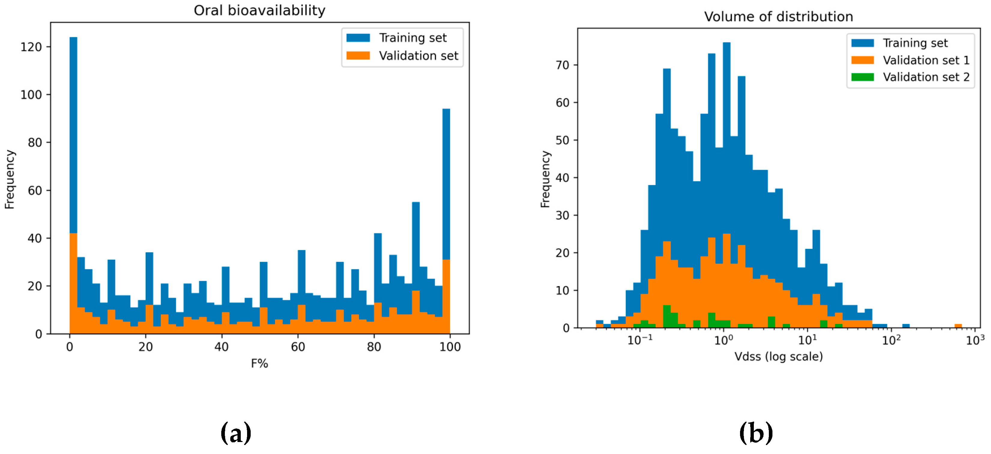
Figure 2.
(a) UMAP representation of the chemical space in a 2D map projection for the oral bioavailability dataset. Each point represents a chemical, and its color encodes the corresponding F% value, ranging from red for low oral bioavailability to blue for high oral bioavailability. (b) UMAP representation of the chemical space in a 2D map projection for the VDss dataset. Points are colored considering the Log transformed VDss values from red to blue for low to high VDss.
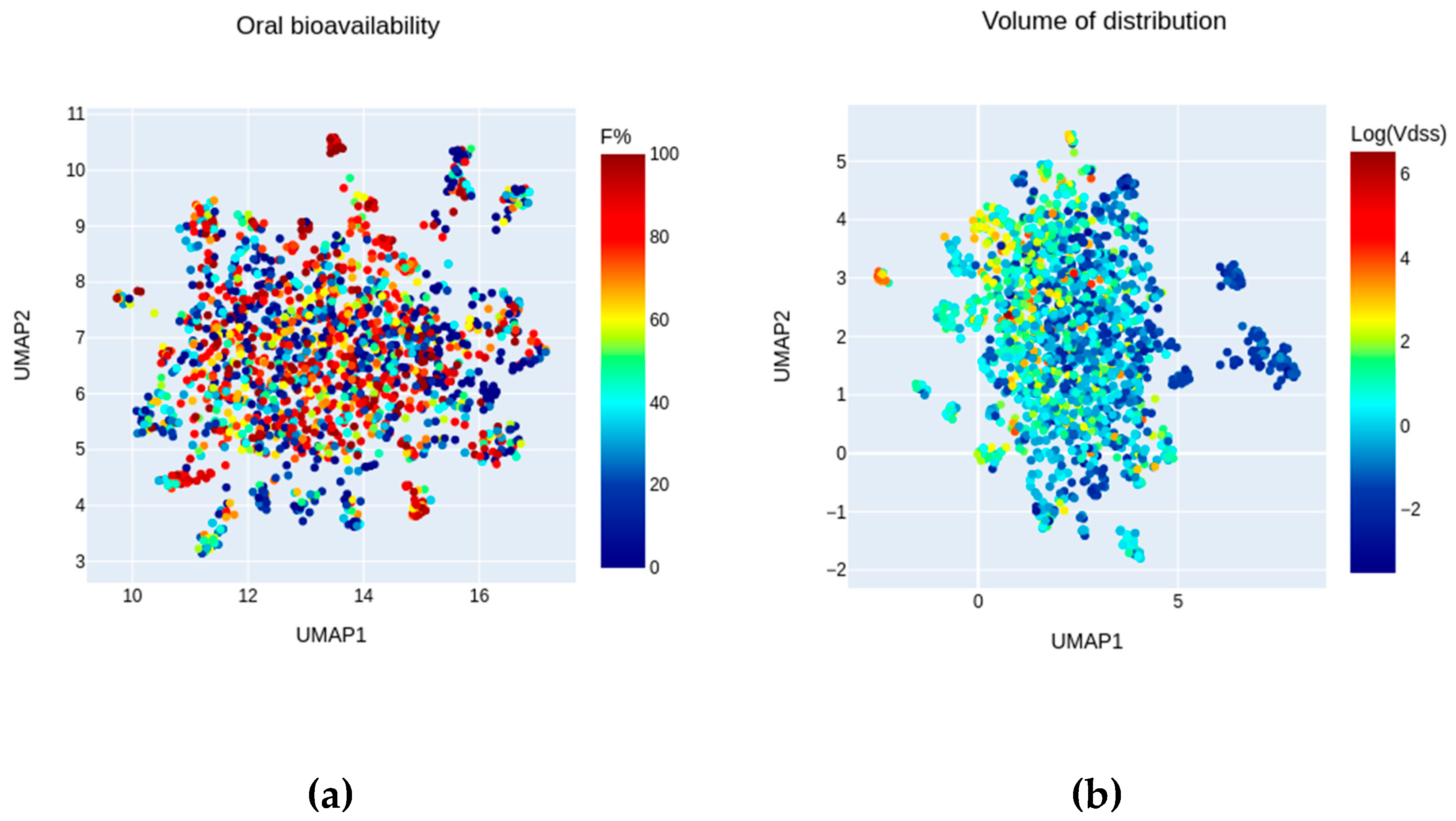
Figure 3.
Effect on coverage and predictive performance of different definitions of applicability domains. (a) 3-NN Tanimoto AD. Evolution of the Q²F3 performance between observed and predicted values (red) on the validation set between predicted and real values according to different Tanimoto thresholds ranging from 0 to 1. The evolution of the validation set coverage is plotted as blue bars. The model tested is the regression CatBoost method predicting F% values. (b) SARpy LR AD. Evolution of the Q²F3 performance (red) on the validation set according to different Log ratio thresholds relative to the structural alert associated with query chemicals. The evolution of the validation set coverage is plotted as blue bars.
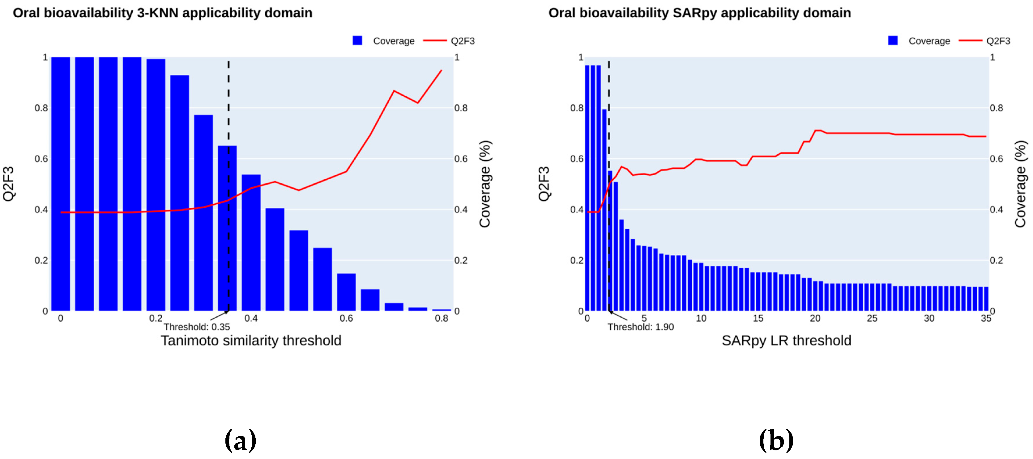
Figure 4.
Effect on coverage of the validation set 1 and predictive performance of different definitions of applicability domains (a) 3-NN Tanimoto AD. Evolution of the GMFE (in red) on the validation set 1 according to different Tanimoto thresholds ranging from 0 to 1. The evolution of the coverage of the validation set is plotted as blue bars. (b) SARpy AD. Evolution of the GMFE performance (in red) on the validation set according to different Log ratio thresholds relative to the structural alert associated with the prediction. The evolution of the effective size retained in the validation set is plotted alongside in blue. The plot is made using the SARpy model with the 0.6-5 L/Kg threshold.
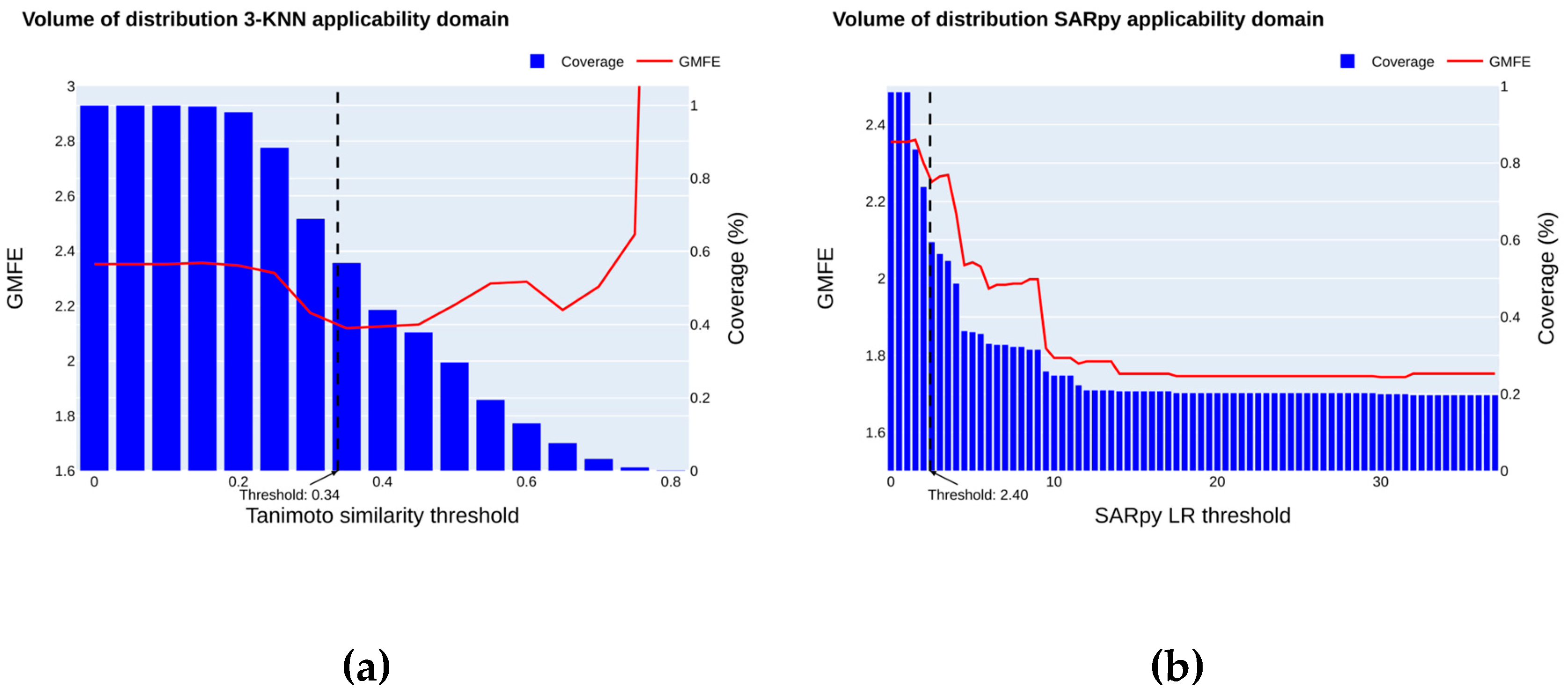
Figure 5.
(a) Summary plot obtained by using the SHAP package. The plot shows the importance of the 15 most important molecular descriptors of the R-CatBoost (regression) oral bioavailability model and their effect on the predictions. The plot enables the observation of the relationship between a molecular descriptor's value and its impact on the prediction. For instance, high values of jGI9 (a topological charge molecular descriptor) are associated with a tendency to decrease oral bioavailability. (b) Summary plot obtained by using the SHAP package of the R-RF (regression) VDss model. The plot shows the importance of the 15 most important molecular descriptors and their effect on the predictions. This plot enables the observation of the relationship between a molecular descriptor value and its impact on the prediction. For example, high values of SLogP tend to increase the VDss.
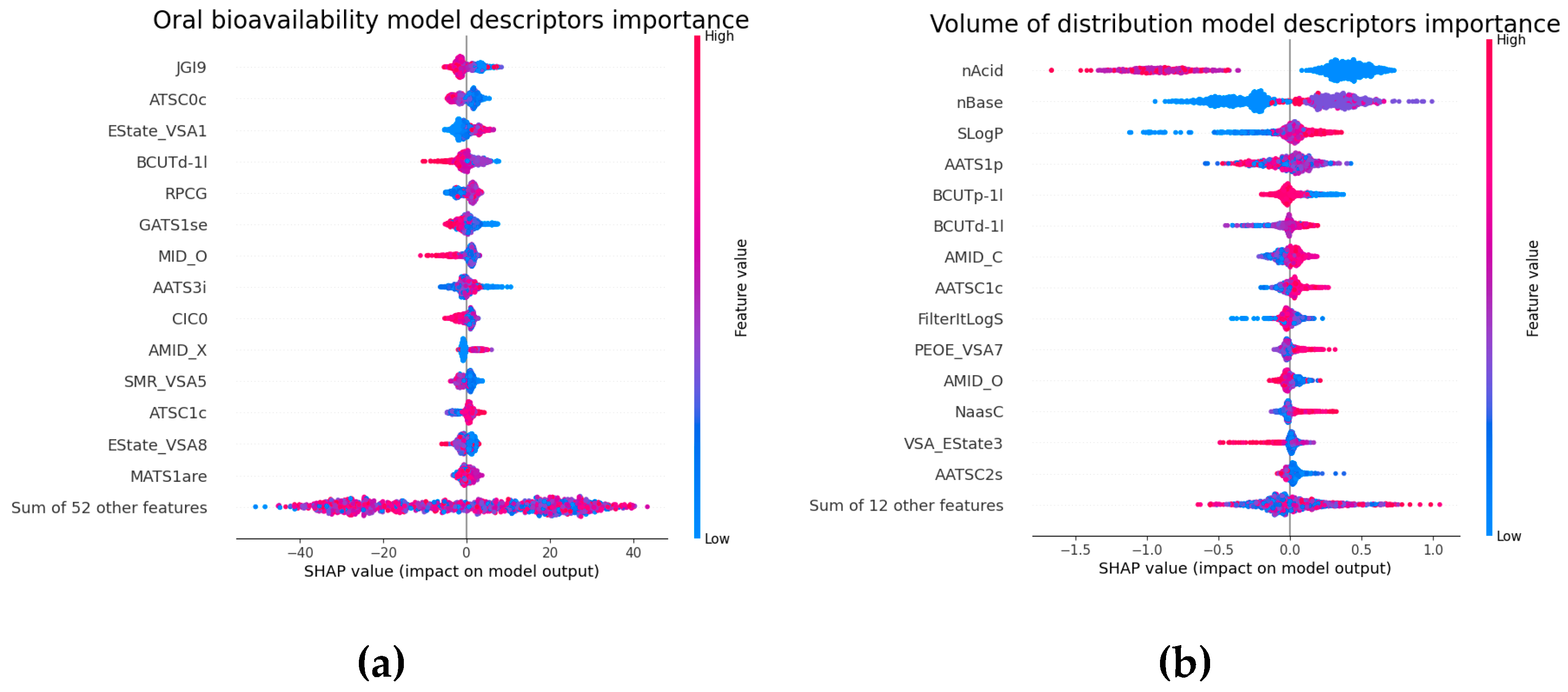
Figure 6.
Boxplot of the predictions for oral bioavailability, VDss and elimination half-life for a set of 131 EDC categorized by 10 chemical categories. Perfluoroalkylcarboxylicl acids (PFCAs), Perfluoroalkylsulfonic acids (PFSAs), Perfluoroalkylether acids (PFEAs), Perfluoroalkane sulfonamide derivatives (PASFs), Perfluoroalkyl phosphonic acids (PFPiAs), Polyfluoroalkyl phosphate diesters (diPAPs) categories were grouped as PFASs. Chemicals inside the SARpy AD were represented as circles, and chemicals outside as crosses. Background color was set to green, orange and red for respectively low, medium and high values of VDss (Thresholds: 0.6Kg/L and 5 Kg/L), oral bioavailability (Thresholds: 30% and 60%) and elimination half-life (Thresholds: 4h and 24h).
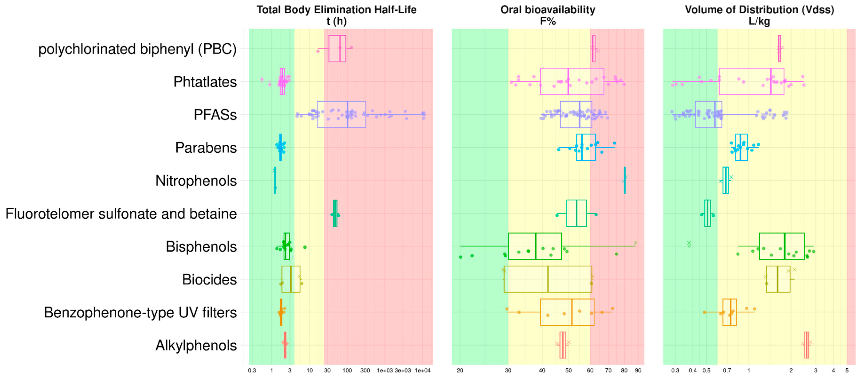
Figure 7.
Structural fragment alerts identified by MC-SARpy in more than two chemicals across different EDC categories for the VDss (a) and oral bioavailability (b) models. The Log ratio and the predicted category associated with each structural alert are reported. PASFs, PFCAs, PFEAs, PFSAs, diPAPs, PFPiAs were combined into the PFASs category when the structural fragment was identical.
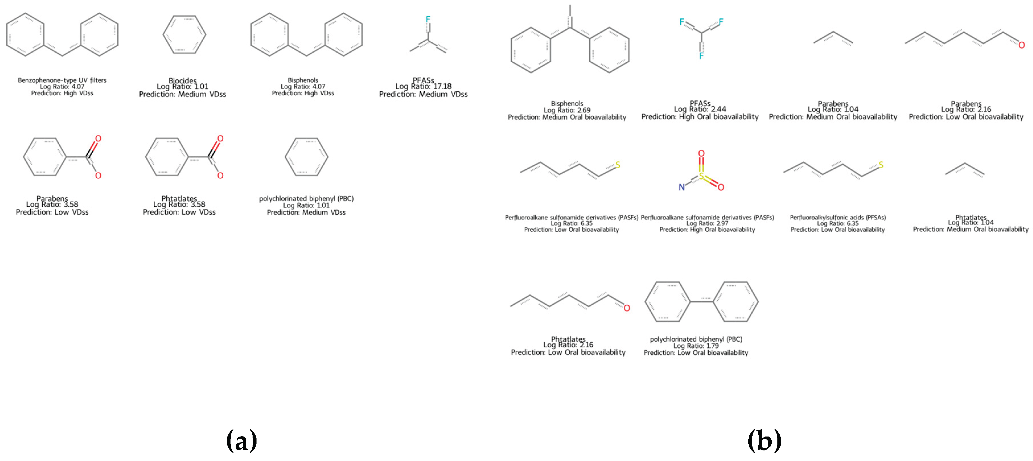

Table 1.
Number of chemicals used for developing QSAR models, according to the specified algorithms, for oral bioavailability and for VDss. It is noted that there are more chemicals for the single threshold and the double thresholds modeling, since some data sources provided data with qualifiers for F%.
| Endpoint | Dataset | Modeling algorithm | # Chemicals |
|---|---|---|---|
| Oral bioavailability | Training | Regression | 1213 |
| Classification (50% threshold) | 1307 | ||
| Binary Classification (30%,60% thresholds) | 1244 | ||
| Validation | Regression/ Binary Classification/ Multiclass Classification | 405 | |
| VDss | Training | Regression/Binary Classification/Multiclass Classification | 1167 |
| Validation 1 | 390 | ||
| Validation 2 | 34 |
Table 2.
Performances obtained for the QSAR models predicting oral bioavailability on the validation set. The predictive performance of the algorithms was evaluated across regression (R), binary classification (BC), and multiclass classification (MC) tasks.
Table 2.
Performances obtained for the QSAR models predicting oral bioavailability on the validation set. The predictive performance of the algorithms was evaluated across regression (R), binary classification (BC), and multiclass classification (MC) tasks.
| Metric | Performance for regression (R) | Performance for binary classification (BC) | Performance for multiclass classification (MC) | CV Performance for regression (R) | CV Performance for binary classification (BC) | CV Performance for multiclass classification (MC) |
|---|---|---|---|---|---|---|
| Validation set | CV | |||||
| Model | R-CatBoost | BC-CatBoost | MC-CatBoost | R-CatBoost | BC-CatBoost | MC-CatBoost |
| Regression metrics | ||||||
| RMSE | 25.86 | NA | 27.71±0.98 | |||
| R² | 0.42 | NA | NA | 0.38±0.04 | NA | NA |
| MAE | 20.09 | NA | NA | 20.90±0.82 | NA | NA |
| MedAE | 15.92 | NA | NA | 17.01±1.11 | NA | NA |
| Q²F3 | 0.39 | NA | NA | 0.34±0.05 | NA | NA |
| Binary Classification metrics | ||||||
| Sensitivity | 0.78 | 0.79 | NA | 0.75±0.03 | 0.78±0.03 | NA |
| Specificity | 0.76 | 0.68 | NA | 0.72±0.03 | 0.69±0.04 | NA |
| Balanced accuracy | 0.77 | 0.74 | NA | 0.74±0.02 | 0.74±0.02 | NA |
| Multiclass Classification metrics | ||||||
| Sensitivity (<30%) | 0.46 | NA | 0.67 | 0.45±0.05 | NA | 0.64±0.05 |
| Specificity (<30%) | 0.91 | NA | 0.86 | 0.93±0.03 | NA | 0.83±0.03 |
| Balanced accuracy (<30%) | 0.68 | NA | 0.77 | 0.63±0.02 | NA | 0.74±0.02 |
| Sensitivity [30%-60%] | 0.58 | NA | 0.25 | 0.69±0.02 | NA | 0.31±0.05 |
| Specificity [30%-60%] | 0.63 | NA | 0.89 | 0.63±0.03 | NA | 0.88±0.02 |
| Balanced accuracy [30%-60%] | 0.60 | NA | 0.57 | 0.63±0.03 | NA | 0.60±0.03 |
| Sensitivity (>60%) | 0.63 | NA | 0.83 | 0.63±0.04 | NA | 0.79±0.03 |
| Specificity (>60%) | 0.84 | NA | 0.67 | 0.84±0.03 | NA | 0.70±0.03 |
| Balanced accuracy (>60%) | 0.74 | NA | 0.75 | 0.74±0.02 | NA | 0.74±0.02 |
| Macro Sensitivity | 0.56 | NA | 0.58 | 0.57±0.03 | NA | 0.58±0.02 |
| Macro Specificity | 0.79 | NA | 0.81 | 0.80±0.01 | NA | 0.81±0.01 |
| Macro Balanced accuracy | 0.68 | NA | 0.70 | 0.68±0.02 | NA | 0.69±0.02 |
| Micro Sensitivity | 0.56 | NA | 0.64 | 0.57±0.03 | NA | 0.63±0.02 |
| Micro Specificity | 0.78 | NA | 0.82 | 0.79±0.01 | NA | 0.82±0.01 |
Table 3.
Predictive performance for the QSAR models for the prediction of VDss as a function of the validation set 1. The predictive performance of the algorithms was evaluated across regression (R), binary classification (BC), and multiclass classification (MC) tasks.
Table 3.
Predictive performance for the QSAR models for the prediction of VDss as a function of the validation set 1. The predictive performance of the algorithms was evaluated across regression (R), binary classification (BC), and multiclass classification (MC) tasks.
| Metric | Regression model performance | Classification model performance | Classification multiclass model performance | CV Regression model performance | CV Classification model performance | CV Classification multiclass model performance |
|---|---|---|---|---|---|---|
| Validation set 1 | CV | |||||
| Model | R-RF | BC-Chemprop | MC-Chemprop | R-RF | BC-Chemprop | MC-Chemprop |
| Regression metrics | ||||||
| GMFE | 2.35 | NA | NA | 2.19±0.08 | NA | NA |
| Binary Classification metrics | ||||||
| Sensitivity | 0.79 | 0.77 | NA | 0.79±0.03 | 0.73±0.06 | NA |
| Specificity | 0.71 | 0.75 | NA | 0.75±0.03 | 0.83±0.04 | NA |
| Balanced accuracy | 0.75 | 0.76 | NA | 0.77±0.02 | 0.78±0.03 | NA |
| Multiclass Classification metrics | ||||||
| Sensitivity (<0.6) | 0.62 | NA | 0.68 | 0.66±0.04 | NA | 0.71±0.05 |
| Specificity (<0.6) | 0.91 | NA | 0.76 | 0.90±0.02 | NA | 0.87±0.03 |
| Balanced accuracy (<0.6) | 0.76 | NA | 0.45 | 0.78±0.02 | NA | 0.79±0.03 |
| Sensitivity [0.6-5] | 0.82 | NA | 0.89 | 0.83±0.03 | NA | 0.76±0.05 |
| Specificity [0.6-5] | 0.51 | NA | 0.63 | 0.57±0.04 | NA | 0.66±0.05 |
| Balanced accuracy [0.6-5] | 0.67 | NA | 0.94 | 0.70±0.02 | NA | 0.71±0.03 |
| Sensitivity (>5) | 0.22 | NA | 0.78 | 0.32±0.06 | NA | 0.42±.09 |
| Specificity (>5) | 0.97 | NA | 0.70 | 0.97±0.01 | NA | 0.94±0.02 |
| Balanced accuracy (>5) | 0.60 | NA | 0.69 | 0.64±0.03 | NA | 0.68±0.04 |
| Macro Sensitivity | 0.56 | NA | 0.63 | 0.60±0.03 | NA | 0.63±0.03 |
| Macro Specificity | 0.80 | NA | 0.82 | 0.81±0.01 | NA | 0.82±0.02 |
| Macro Balanced accuracy | 0.68 | NA | 0.72 | 0.71±0.02 | NA | 0.73±0.02 |
| Micro Sensitivity | 0.65 | NA | 0.68 | 0.68±0.02 | NA | 0.69±0.03 |
| Micro Specificity | 0.83 | NA | 0.84 | 0.84±0.01 | NA | 0.84±0.01 |
| Micro Balanced accuracy | 0.74 | NA | 0.76 | 0.76±0.02 | NA | 0.77±0.02 |
Disclaimer/Publisher’s Note: The statements, opinions and data contained in all publications are solely those of the individual author(s) and contributor(s) and not of MDPI and/or the editor(s). MDPI and/or the editor(s) disclaim responsibility for any injury to people or property resulting from any ideas, methods, instructions or products referred to in the content. |
© 2025 by the authors. Licensee MDPI, Basel, Switzerland. This article is an open access article distributed under the terms and conditions of the Creative Commons Attribution (CC BY) license (http://creativecommons.org/licenses/by/4.0/).
Copyright: This open access article is published under a Creative Commons CC BY 4.0 license, which permit the free download, distribution, and reuse, provided that the author and preprint are cited in any reuse.


