
Submitted:
27 August 2025
Posted:
27 August 2025
You are already at the latest version
Abstract
This article introduces the main characteristics of PyMossFit, a software for Mössbauer spectra fit. It is explained how each utility of their code sections works. Based on the Lmfit python package, it is a robust data fitting tool. Designed to run as a Jupyter notebook at the Google Colab cloud, it also allows us to work from multiple devices and operating systems. Additionally, it facilitates that fitting procedure can be performed in a collaborative way by researchers.The software performs the folding of raw data with a discrete Fourier transform. Data smoothing is available with the use of a Savitzky-Golay algorithm. Likewise, a K-nearest neighbor algorithm helps us to determine the present phases by matching the correlations of hyperfine parameters from a local database.
Keywords:
Cloud Computing
; Mössbauer Effect Spectroscopy
; Condensed Matter Physics
; Python
1. Introduction
Mössbauer effect spectroscopy [1,2] is a highly specialized technique that investigates the resonant absorption of rays by atomic nuclei. The Mössbauer effect, observed primarily in isotopes such as iron-57 (57), provides information on hyperfine interactions, including isomer shifts, quadrupole splittings, and magnetic hyperfine fields. These parameters offer detailed information on the electronic, magnetic and structural environment of the sample, making the technique invaluable in materials science, condensed matter physics, chemistry, biology [3], planetary science [4], and also in cosmology [5]. The gamma ray of resonant absorption in 57 nuclei is 14.4 keV and hyperfine interactions promote the break of degeneracy at ground and excited nuclear levels. The above cited parameters are described in the following subsections:
1.1. Isomer Shift, or
This phenomenon corresponds to a certain probability that electrons have to be inside the nucleus [6], an exclusive quantum event. The next equation describes this parameter.
where , are the s-wavefunctions at the origin of the absorbent (A) and the -ray source (S) nucleus, while is the relative nuclear radius R change during recoilless resonant absorption.
1.2. Quadrupole Splitting, or
This quantum effect gives account of the interaction of nuclear charge with an electric field gradient (EFG) originated in an asymmetric electronic orbital distribution. The analytical expression is
being Q the quadrupolar moment, the principal component of the EFG, and the asymmetric factor.
1.3. Magnetic Hyperfine Field,
Nucleons have an intrinsic quantum property, the spin. When the spin is coupled with the quantum orbital moment, a total moment can interact with the local magnetic field induced by the electronic orbitals, giving rise to a more complex splitting (Zeeman effect) and, according to the nuclear selection rules with some forbidden transitions, and consequently, certain decays by -ray emission are not physically possible.
The Figure 1 shows the energy levels schemes of all of these hyperfine interactions for the 57 isotope. As can be observed, IS shifts the excited and ground energy levels between the source nucleus and the sample one; meanwhile, QS promotes the splitting of the excited level and the same in both the ground and excited levels, with the and forbidden transitions by the selection rules.
In a typical Mössbauer experiment, a radioactive source emits gamma rays, which are absorbed by the nuclei in the sample (see Figure 2). Resonant absorption occurs, in a small fraction, when rays hit the probe with recoilless. The detector measures the intensity of the transmitted radiation as a function of the velocity of the gamma-ray source (with an additional energy added by Doppler effect). This results in a Mössbauer spectrum, typically characterized by sharp peaks or dips at resonance frequencies corresponding to different hyperfine interactions within the sample. The most common experimental setup corresponds to Transmission Geometry (in this case, the observed lines come from a reduction of 14.4 keV gamma counting in the detector, as compared to the background signal). Another possible option is the Backscattering Mössbauer Spectroscopy (BMS) which corresponds to detection of back-scattered electrons after gamma absorption. In recent years, the use of synchrotron radiation was extended, helping to collect Mössbauer spectra with deeper details and in a short time [7].
1.4. Statement of Need
Recently, in a review by Grandjean et al. [8], the authors made a series of suggestions about how good measurements should be taken, which could be a good practice for Mössbauer data treatment and its corresponding fitting presentation. Usually, scientists working with Mössbauer spectroscopy manage their data and fit them with non-open source software that runs on a Windows OS with poor upgrade services [9]. The needs of an open source option with less OS or package dependency has motivated this work.
In this sense, Google Colab is a useful tool for a collaborative team job in data analysis with the advantage of no additional packages locally installed, also compatible with the fact that the user can run their codes from multiple devices.
2. Mössbauer Spectra and Curve Shapes
The shape of a Mössbauer spectrum varies depending on the nature of the hyperfine interactions in the sample. For example, a simple paramagnetic material might produce a single absorption peak (Lorentzian or Gaussian) due to the isomer shift. Materials with quadrupole splitting generate a doublet (two peaks), while materials experiencing magnetic hyperfine interactions often exhibit more complex sextet patterns. These spectral features often overlap, making it difficult to isolate and quantify each individual component.
2.1. Curve Fitting and Least Squares Method
Curve fitting plays a crucial role in Mössbauer spectral analysis, as it allows for the decomposition of these complex spectra into individual contributions, each associated with specific hyperfine parameters. The challenge lies in accurately reproducing the spectral shapes using mathematical models and adjusting the parameters until a satisfactory fit is achieved.
To accurately extract physical parameters from Mössbauer spectra, fitting procedures are applied to the experimental data. One of the most common approaches is the least squares method, which minimizes the difference between the experimental data points and the theoretical model curve. The objective is to adjust the parameters of the theoretical model (such as isomer shift, quadrupole splitting, and line broadening) so that the calculated spectrum fits the experimental data as closely as possible. Then, a minimization of the is defined as:
beeing a set of selected parameters for fitting, which minimizes the distance between the experimental data, and the modeled data points .
In Python, this process can be implemented using libraries like Lmfit [10], SciPy [11], or NumPy [12], which provide robust tools for processing data, graphics, and least-squares curve fit. The general approach involves defining a model function that represents the expected shape of the Mössbauer spectrum, which could be a sum of multiple Lorentzian or Gaussian functions, depending on the number and type of spectral components. Lorentzian functions are preferred with crystalline samples, whereas PseudoVoigts (sum of Lorentzian and Gaussian functions) are appropriate for Fe sites in disordered materials.
The least-squares fitting algorithm iteratively adjusts the model parameters until the sum of squared residuals between the experimental and calculated spectra is minimized. An example of a Lorentzian function definition for Python, can be seen next,
⠀
from scipy.optimize import curve_fit
import numpy as np
⠀
# Define the model function (e.g., a sum of Lorentzian components)
def lorentzian(x, amplitude, center, width):
return amplitude * (width**2 / ((x - center)**2 + width**2))
⠀
# Generate synthetic data for fitting
x_data = np.linspace(-10, 10, 500) # Example velocity range
y_data = lorentzian(x_data, 1, 0, 1) + np.random.normal(0, 0.02,
size=len(x_data))
⠀
# Perform least-squares curve fitting
initial_guess = [1, 0, 1] # Initial guess for parameters
params, covariance = curve_fit(lorentzian, x_data, y_data,
p0=initial_guess)
⠀
# params contains the optimized parameters: amplitude, center,
and width
⠀
This example demonstrates fitting a single Lorentzian function to synthetic data, though more complex models involving sums of Lorentzians or other spectral shapes can be implemented to represent real Mössbauer spectra.
3. Description of the Python code for Google Colab (PyMossFit)
The Python code is available in several Jupyter notebooks as typical examples found in practice [13]. In their names, some text is added that indicates the number and type of interactions (i. e. 1Q means one quadrupolar interaction, 2X for two magnetic sites, and so on). Some selected parts of it are described throughout this page.
The code is structured in three cells. The first includes the installation in the Google Colab environment of Lmfit, the core of data fitting. Likewise, it imports some packages of Scipy, Pandas, Matplotlib and Numpy, among others. The next step includes a Drive connection that asks the user for permission.
The second cell reads the datafile (format should be inspected previously to define "delimiter", "columns" and "skiprows" parameters). The required inputs are date (in a YYYYMMDD format) and maximum velocity associated to the extreme channels, in order to define the velocity scale.
In this cell, spectrum folding is performed with a Discrete Fourier Transforming (DFT) routine, the Numpy fft. The theory of this procedure corresponds to the Nyquist-Shannon Sampling Theorem that helps to determine a folding channel from the symmetry of discrete Fourier spectra [14].
Data can also be smoothed using a Savitsky-Golay package (I use savgol from Scipy). After folding, a new datafile is saved for fit with the use of the next cell.
The next figures illustrate the partial plots of data management with this procedure. This spectrum corresponds to zinc-ferrite nanoparticles obtained by a wet chemical method [15], which present a spinel structure with a tetrahedral site for and a octahedral site for both, and , cations.
When raw data are plotted, they look as shown in Figure 3 the following because of the collection of absorption resonances converted to signals in a single-channel analyzer output, while the source moves back and forth. Figure 4 and Figure 5 show the DFT plot and the final folded spectrum, respectively. In the final folded spectrum, the horizontal sequence of channels was transformed to a scale based on a calibration with a metallic 57 thin foil sample.
The set of physical parameters such as linewidth (), isomer shifts (IS), quadrupole splitting (QS) and magnetic hyperfine field () are calculated after adjusting the amplitud (a), full width at half maximum (b), centroid (m), line shift (d) and line separation (q). The initial set of these parameters can be fitted or fixed by selecting the "True" or "False" options, respectively.
A typical fit report of the output of this cell looks as follows:
Figure 6.
An example of a fit report output of a Jupyter notebook in Google Colab
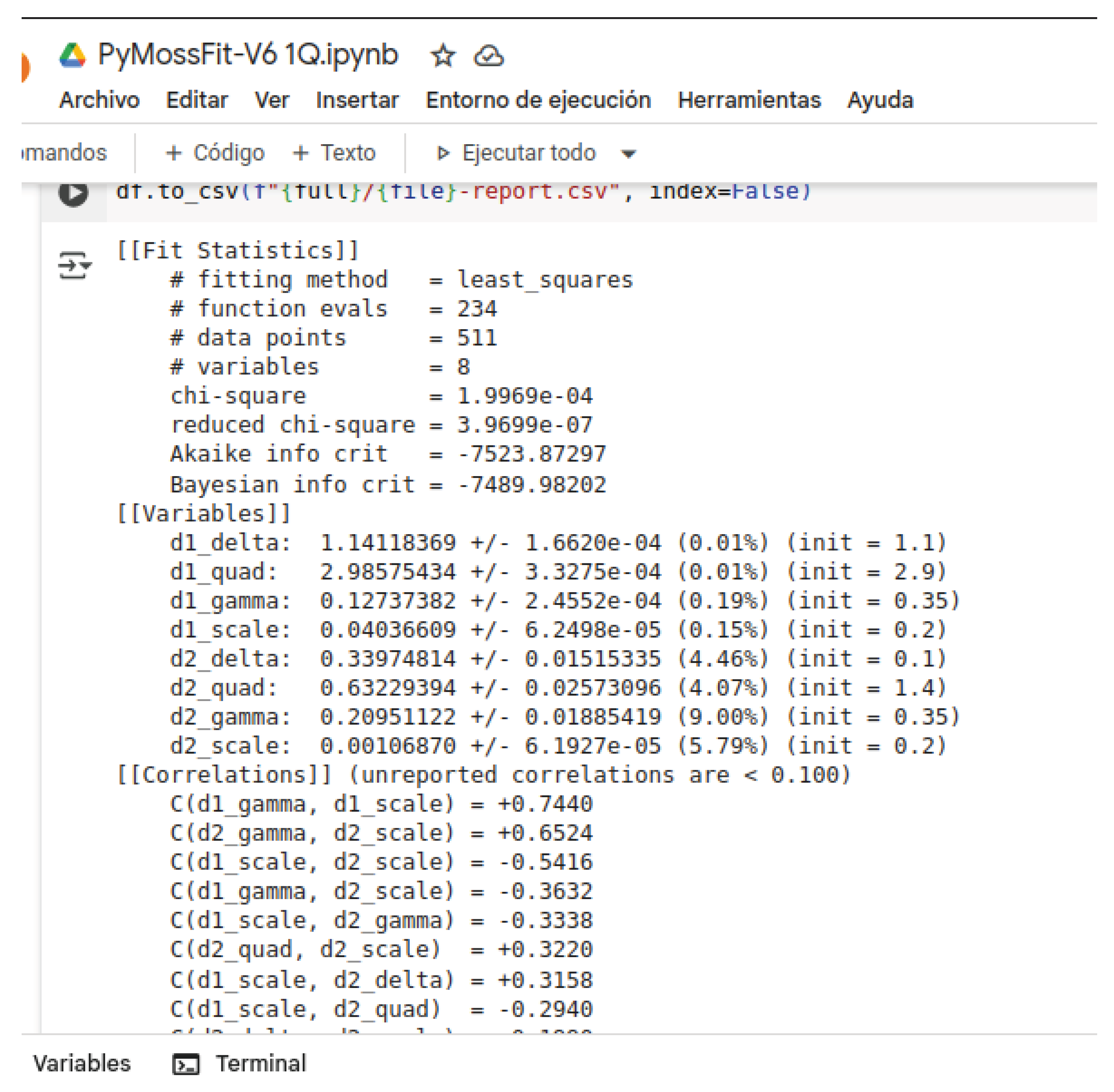
Finally, the code saves fitted parameters, experimental and modeled sub-spectra in CSV formatted output files.
3.1. Some Examples
The following figures illustrate the fit results obtained from the Mössbauer spectra of different samples. Each exhibits several characteristics corresponding to the short-range-order neighborhood of 57 probes. Figure 7 corresponds to the fitted spectrum of an aged cathodic material (LFP) where iron-rich secondary phases can clearly be identified. These undesired phases, which are responsible for the lowering of storage capacity, precipitated after extended thermal and environmental degradation. The fitting procedure took less than 40 secs after an appropriate selection of range parameters.
In contrast, Figure 8 shows a spectrum of a pure LFP sample which was synthesized by a solid-state reaction from analytical grade precursors.
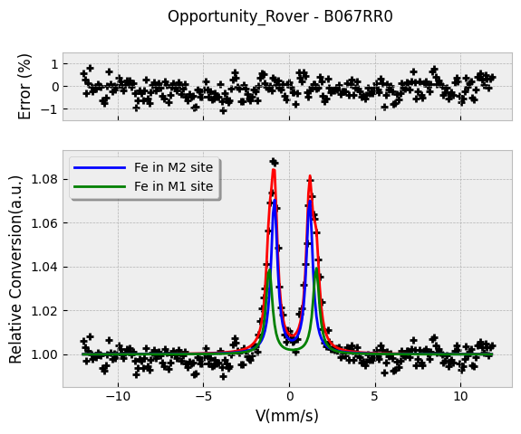
The Figure 9 corresponds to the fitted spectrum with PyMossFit of a soil sample taken by the Mössbauer spectrometer on board the Mars Opportunity Rover. The data is available from [16] and this set is named the "Bounce Rock Case" (B0RR067). The iron-rich detected phase was identified with the code and corresponds to the pyroxene phase (), with two different octahedral Fe sites, M1 and M2 respectively [17,18].
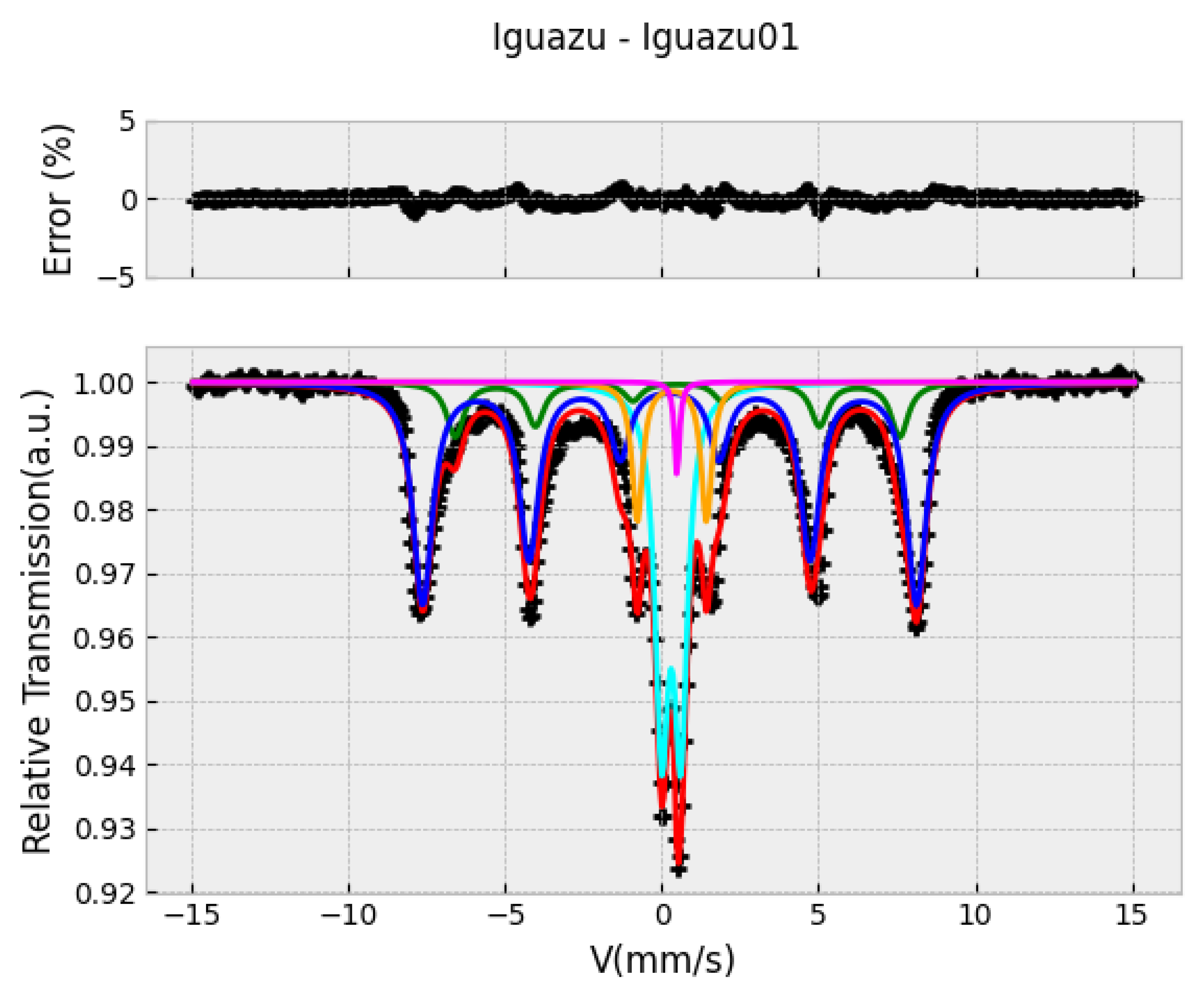
The final example of the use of the PyMossFit notebook is the observed in Figure 10 and is the spectrum of an Iguazú fall soil sample. It corresponds to a complex spectrum where the use of a combination of sextets, doublets, and a singlet was required. All these subspectra correspond to different characteristics of iron oxides and hydroxides present in this kind of soils, originating from the erosion of basalt rocks.
3.2. Match of Fitted Parameters with a Local Database
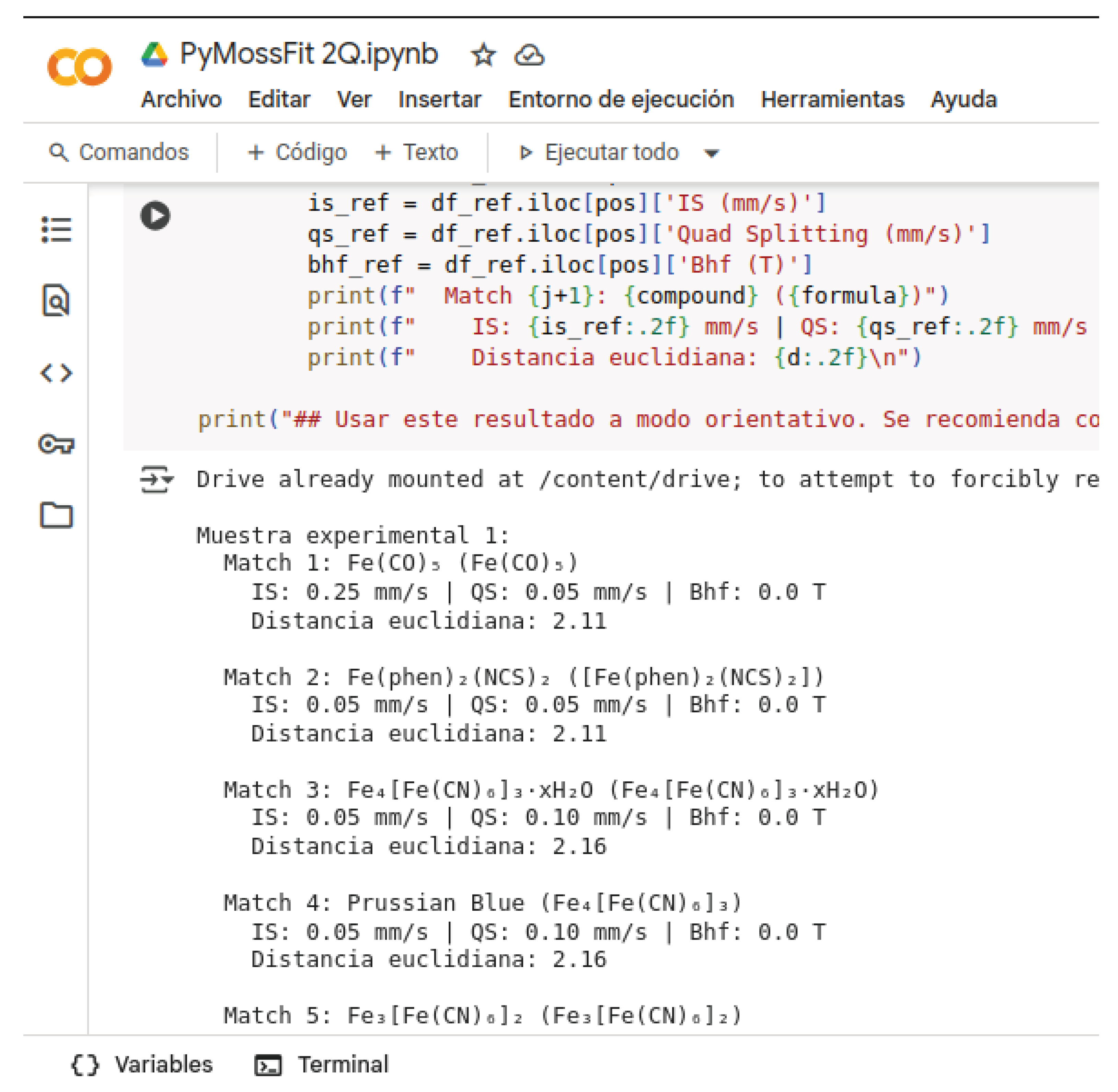
A final cell allows us to identify the phases from an user’s own database or a public ones [19]. This procedure is based on the minimization of Eulerian distances of the set of parameters with the bibliographic collection, which can be updated or extended by the user. Some lines that interpret ranges of hyperfine parameters from the database are also included. The phases cited in the examples above were identified or verified using this code section.
The machine learning algorithm used to guess the present phases is based on a K-Nearest Neighbors (sklearn.neighbors) [20]. The output is a recommendation with a ranking of suggested phases tha match the best.
Figure 11.
A match report obtained with a KNN algorithm for phase identification
4. Conclusions
PyMossFit is a tool for Mössbauer spectroscopy analysis that explodes cloud computing. It was coded in Python and run in Jupyter notebook. The code requires the installation of the Lmfit package as the core of model fitting. PyMossFit was designed to work in Python environment at cloud computing services, such as Google Colab, being a good choice for user update, free OS and device dependencies. Likewise, it simplifies the collaborative work during spectra analysis with the addition of a code section for phase identification based on a KNN algorithm.
Acknowledgments
The author thanks C. P. Ramos from Mōssbauer group of CNEA and the INTECIN(UBA-CONICET) team for sample measurement.
References
- Wikipedia contributors. Mössbauer spectroscopy — Wikipedia, The Free Encyclopedia, 2025. [Online; accessed 19-June-2025].
- Tao, W.; Junhu, Z. The Mössbauer Effect Data Center.
- Martinho, M.; Münck, E., 57Fe Mössbauer Spectroscopy in Chemistry and Biology. In Physical Inorganic Chemistry; John Wiley and Sons, Ltd, 2010; chapter 2, pp. 39–67, [https://onlinelibrary.wiley.com/doi/pdf/10.1002/9780470602539.ch2]. [CrossRef]
- Dyar, M.D.; Agresti, D.G.; Schaefer, M.W.; Grant, C.A.; Sklute, E.C. MÖSSBAUER SPECTROSCOPY OF EARTH AND PLANETARY MATERIALS. Annual Review of Earth and Planetary Sciences 2006, 34, 83–125. [Google Scholar] [CrossRef]
- Gao, Y.; Xu, W.; Zhang, H. A Mössbauer scheme to probe gravitational waves. Science Bulletin 2024, 69, 2795–2798. [Google Scholar] [CrossRef] [PubMed]
- Walker, L.R.; Wertheim, G.K.; Jaccarino, V. Interpretation of the Fe57 Isomer Shift. Phys. Rev. Lett. 1961, 6, 98–101. [Google Scholar] [CrossRef]
- Yi-Long, C.; De-Ping, Y., Synchrotron Mössbauer Spectroscopy. In Mössbauer Effect in Lattice Dynamics; John Wiley and Sons, Ltd, 2007; chapter 7, pp. 253–304, [https://onlinelibrary.wiley.com/doi/pdf/10.1002/9783527611423.ch7]. [CrossRef]
- Grandjean, F.; Long, G.J. Best Practices and Protocols in Mössbauer Spectroscopy. Chemistry of Materials 2021, 33. [Google Scholar] [CrossRef]
- Lagarec, K.; Rancourt, D.G. RECOIL, Mössbauer Spectral Analysis Software for Windows (Version 1.0), 1998.
- Newville, M.e.a. LMFIT: Non-Linear Least-Squares Minimization and Curve-Fitting for Python (version 1.3.4).
- Virtanen, P.; Gommers, R.; Oliphant, T.E.; Haberland, M.; Reddy, T.; Cournapeau, D.; Burovski, E.; Peterson, P.; Weckesser, W.; Bright, J.; et al. SciPy 1.0: Fundamental Algorithms for Scientific Computing in Python. Nature Methods 2020, 17, 261–272. [Google Scholar] [CrossRef] [PubMed]
- Harris, C.R.; Millman, K.J.; van der Walt, S.J.; Gommers, R.; Virtanen, P.; Cournapeau, D.; Wieser, E.; Taylor, J.; Berg, S.; Smith, N.J.; et al. Array programming with NumPy. Nature 2020, 585, 357–362. [Google Scholar] [CrossRef] [PubMed]
- Saccone, F.D. Fitting code for Mössbauer Spectroscopy running in Jupyter Colab, 2025.
- Kong, Q.; Siauw, T.; Bayen, A. Discrete Fourier Transform (DFT), 2020.
- Ferrari, S.; Apehesteguy, J.C.; Saccone, F.D. Structural and magnetic properties of Zn doped magnetite nanoparticles obtained by wet chemical method. IEEE Transactions on Magnetics 2015, 51. [Google Scholar] [CrossRef]
- Opportunity (MERB) Analyst’s Notebook, 2025.
- Corke, P.; Haviland, J. Mössbauer mineralogy of rock, soil, and dust at Meridiani Planum, Mars: Opportunity’s journey across sulfate-rich outcrop, basaltic sand and dust, and hematite lag deposits. Journal of Geophysical Research: Planets 2006, 111. [Google Scholar]
- Oshtrakh, M.I.; Petrova, E.; Grokhovsky, V. Determination of quadrupole splitting for 57Fe in M1 and M2 sites of both olivine and pyroxene in ordinary chondrites using Mössbauer spectroscopy with high velocity resolution. Hyperfine Interactions 2007, 177. [Google Scholar] [CrossRef]
- Tao, W.; Junhu, Z. Mössbauer Effect Data Reference Journal.
- Cover, T.; Hart, P. Nearest neighbor pattern classification. IEEE Transactions on Information Theory 1967, 13, 21–27. [Google Scholar] [CrossRef]
Figure 1.
Energy levels schemes corresponding to Isomer Shift (IS, in blue), ii) Quadrupole Splitting (QS, in red) and iii) Hyperfine Field Splitting with all the allowed transitions (Magnetic Zeeman Effect Field, , in green).
Figure 1.
Energy levels schemes corresponding to Isomer Shift (IS, in blue), ii) Quadrupole Splitting (QS, in red) and iii) Hyperfine Field Splitting with all the allowed transitions (Magnetic Zeeman Effect Field, , in green).
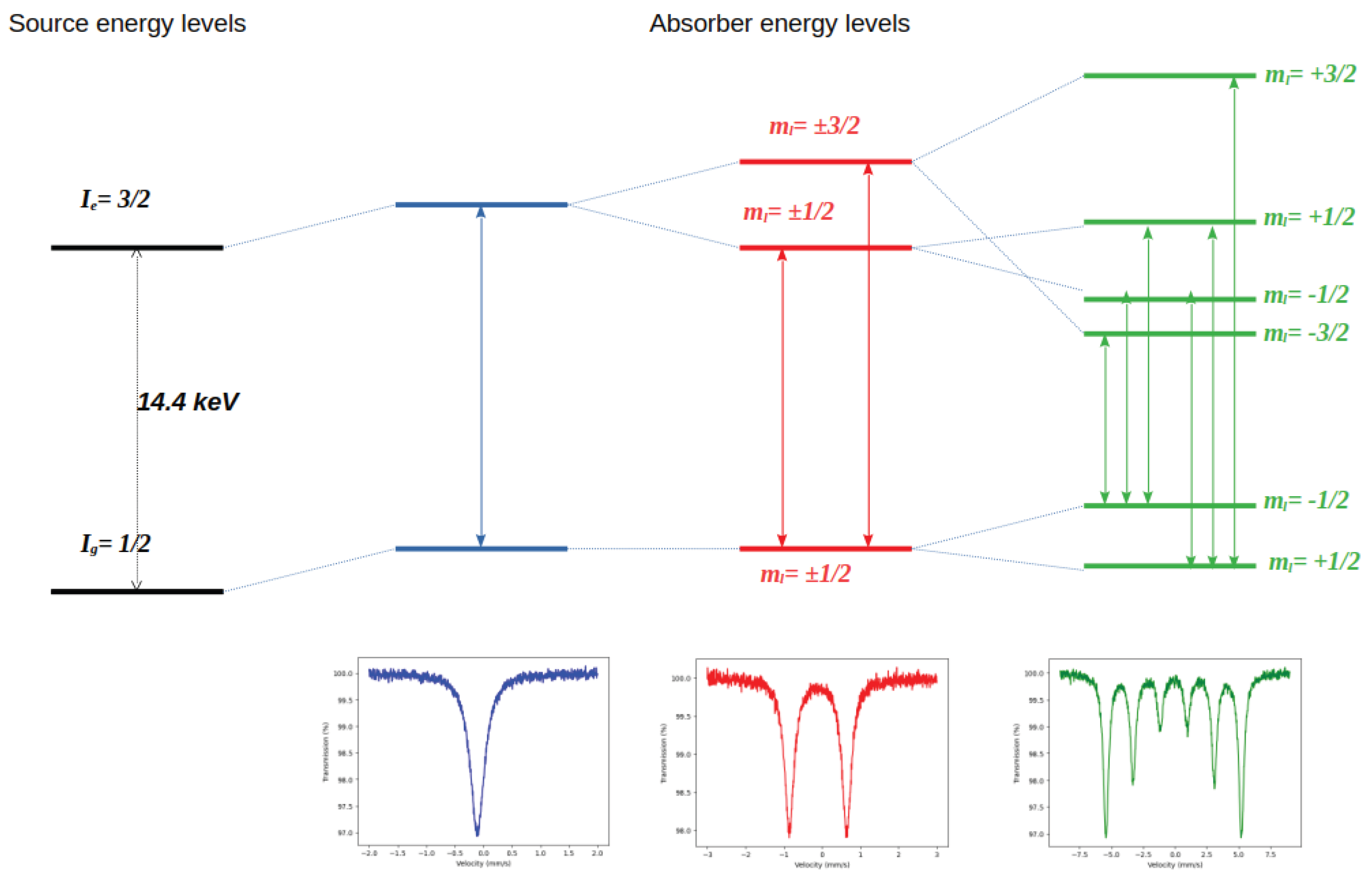
Figure 2.
Scheme of a typical Mossbauer experiment in transmission geometry
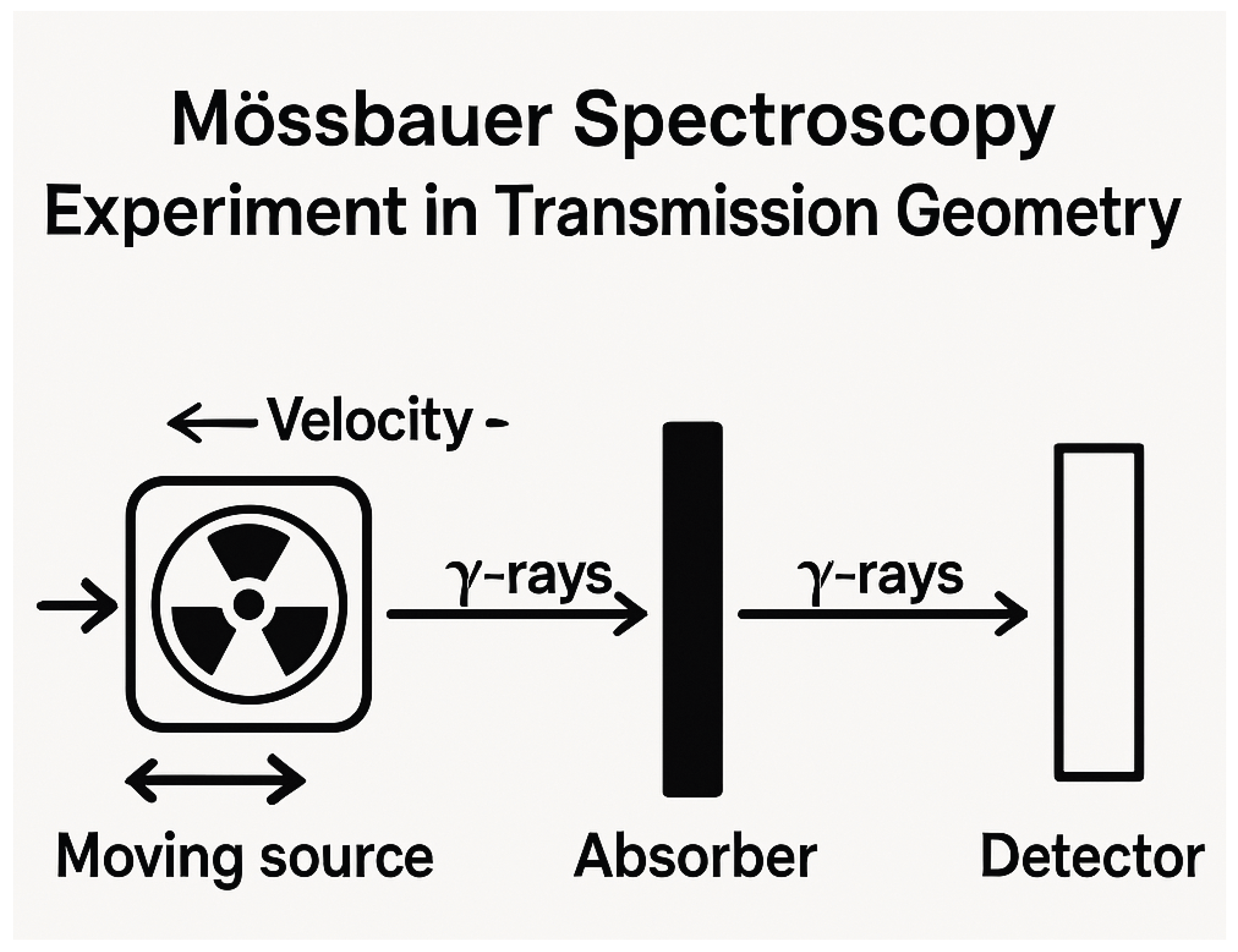
Figure 3.
Unfolded plot of a raw Mossbauer experiment data
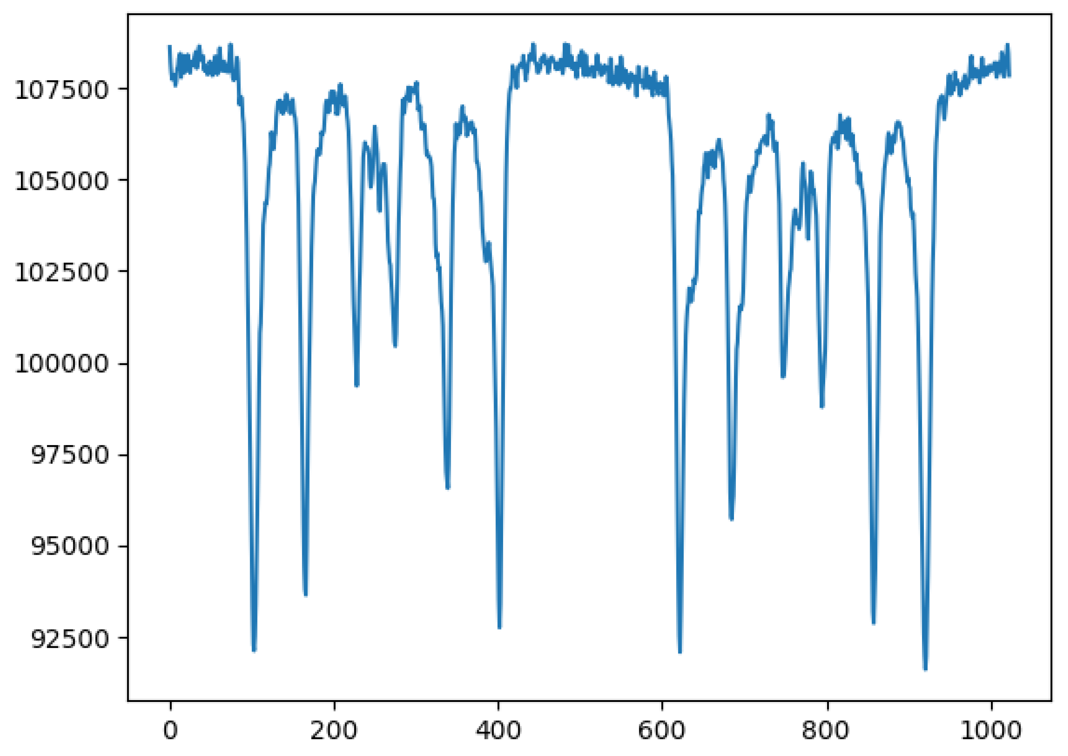
Figure 4.
Discrete Fourier Transform of the raw Mossbauer experiment data ploted in the previous figure
Figure 4.
Discrete Fourier Transform of the raw Mossbauer experiment data ploted in the previous figure
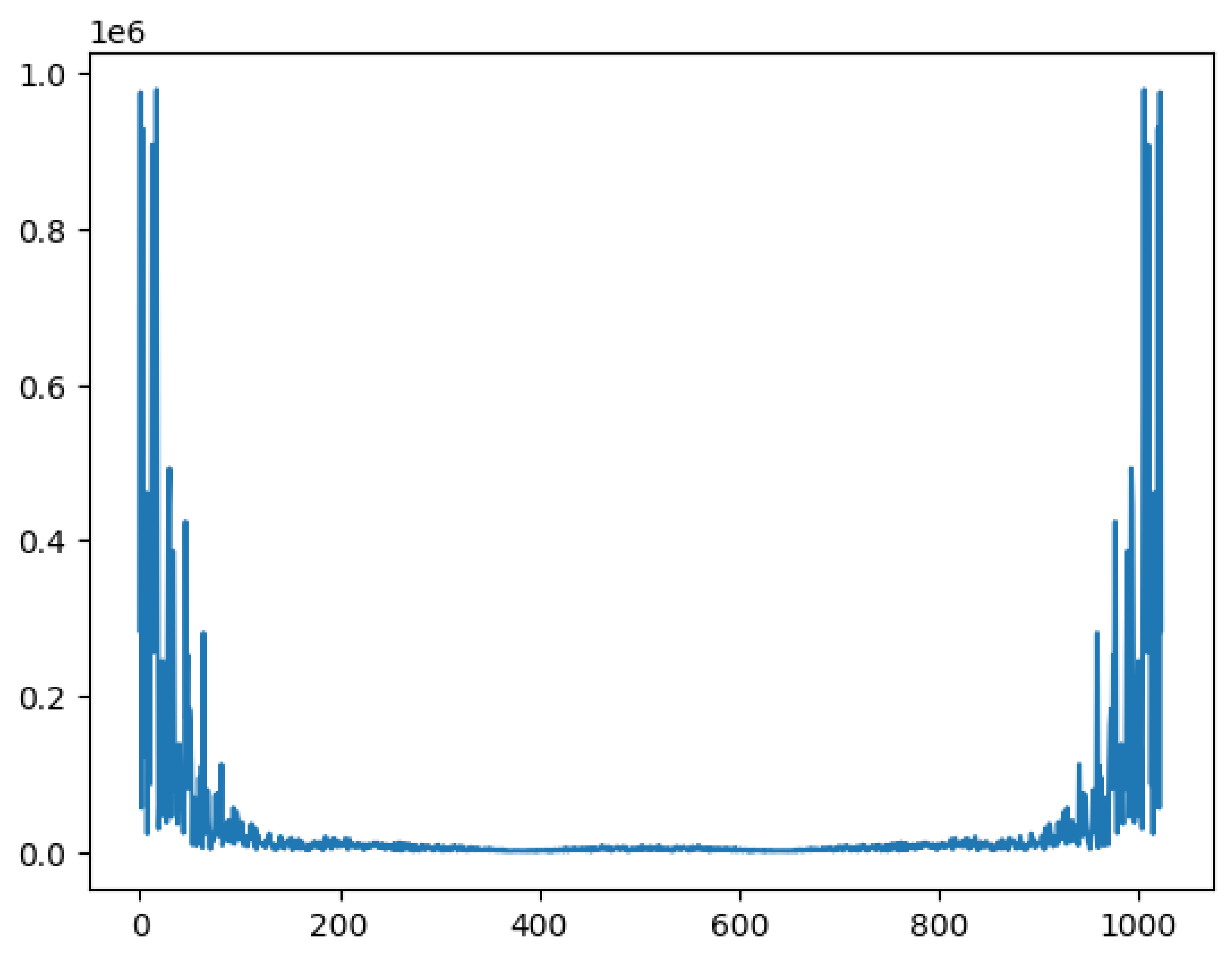
Figure 5.
Final folded spectrum
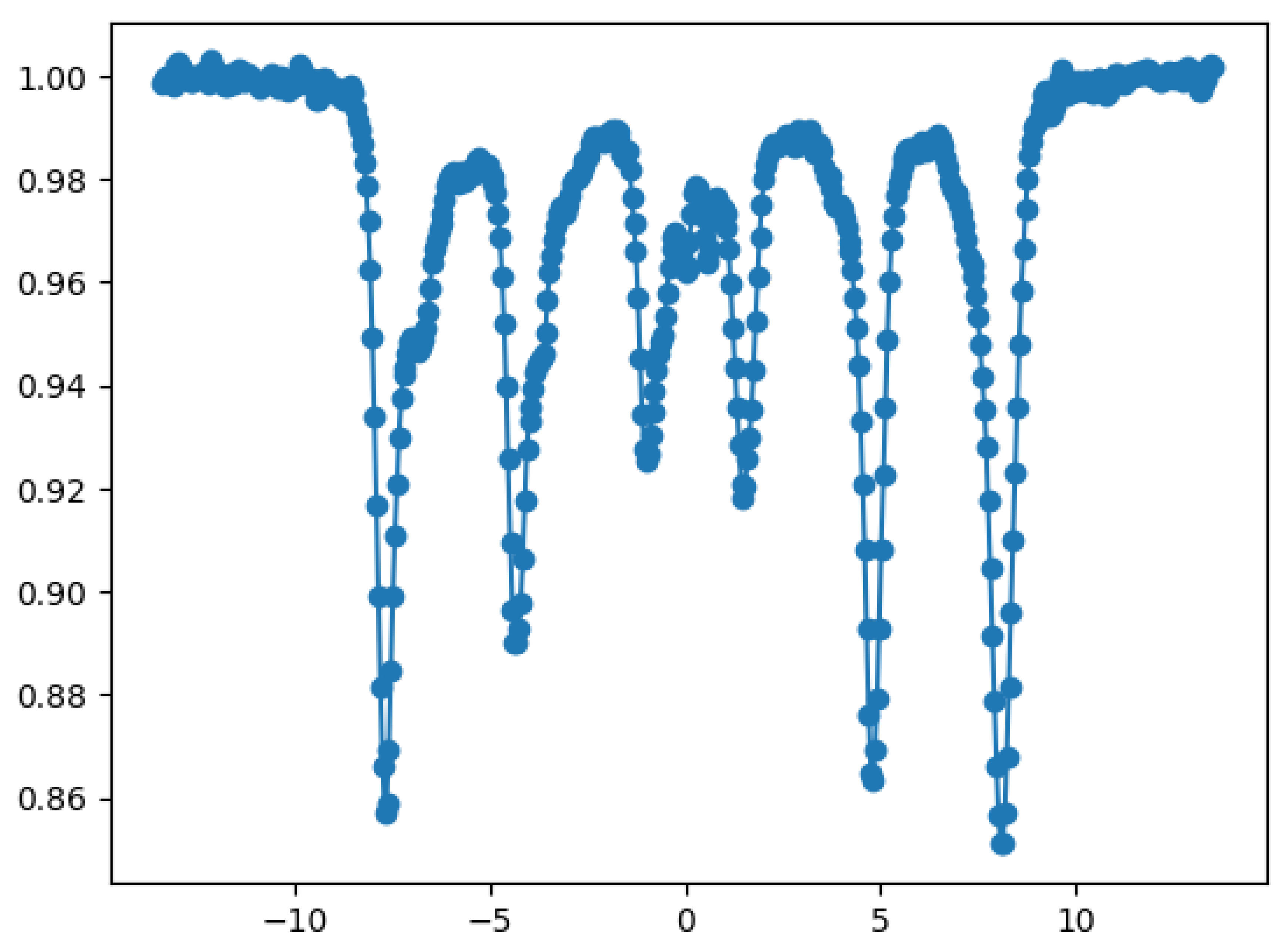
Figure 7.
Mössbauer spectrum of a degraded commercial active material for batteries. Residual phases were detected, such as and . This last phase, shows the presence of 57 in two different oxidation states, and , respectively
Figure 7.
Mössbauer spectrum of a degraded commercial active material for batteries. Residual phases were detected, such as and . This last phase, shows the presence of 57 in two different oxidation states, and , respectively
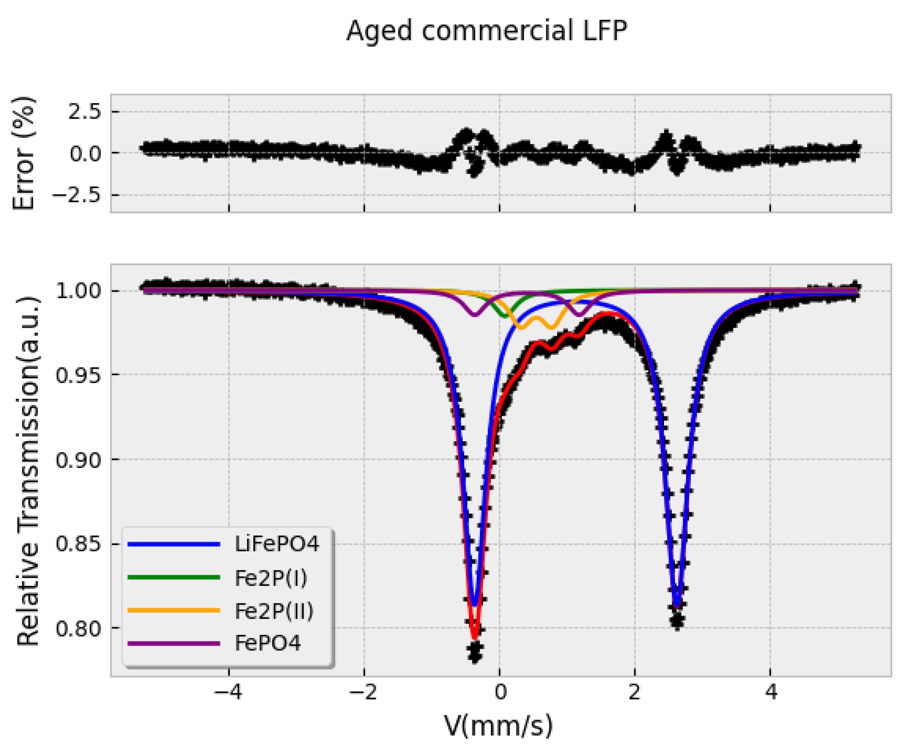
Figure 8.
Mössbauer spectrum of the active material for batteries, after synthesis at lab scale. In this case, just was detected, besides the extraordinary sensitivity of the characterization technique
Figure 8.
Mössbauer spectrum of the active material for batteries, after synthesis at lab scale. In this case, just was detected, besides the extraordinary sensitivity of the characterization technique
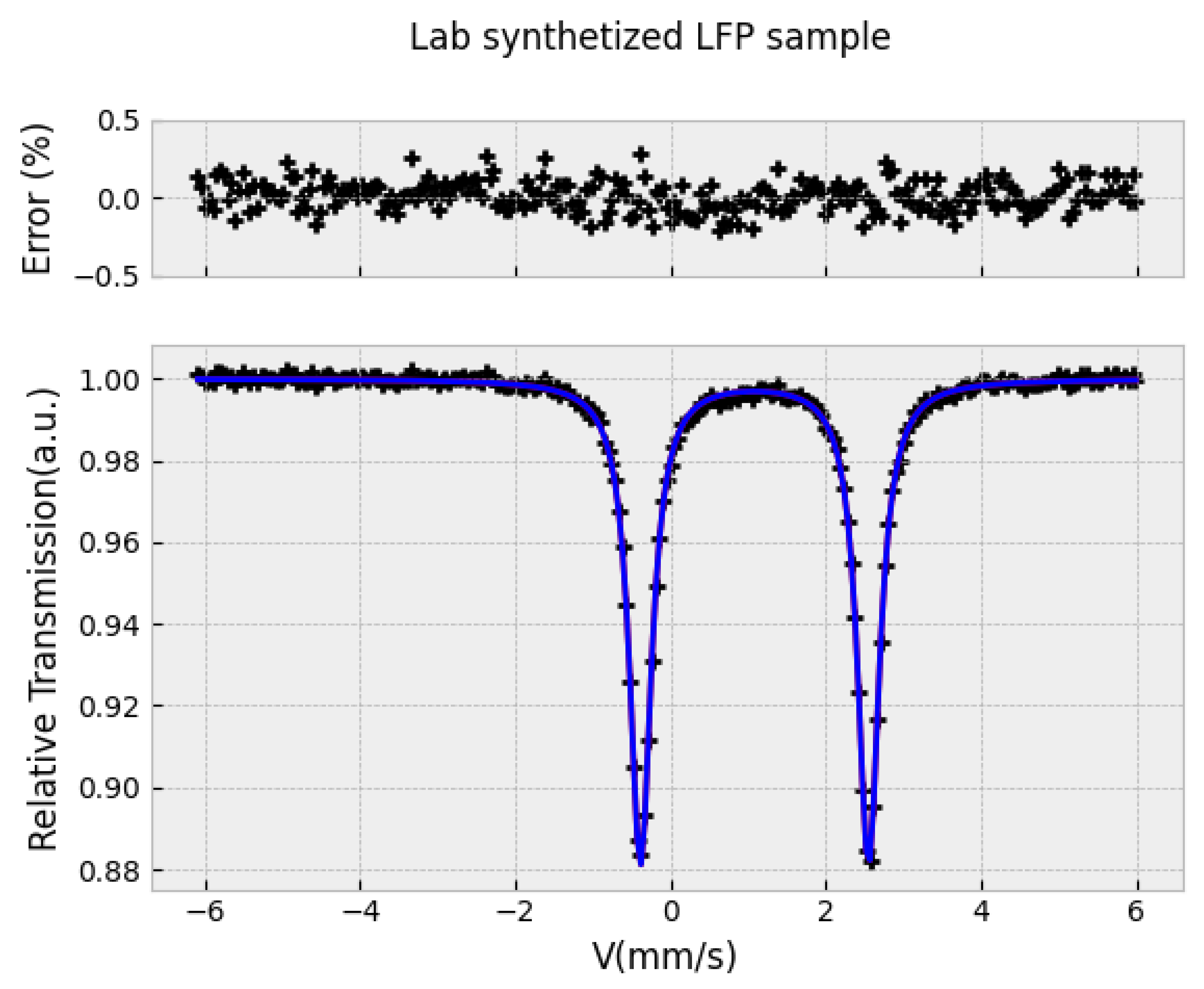
Figure 9.
BMS spectrum of pyroxene in Mars soil (Opportunity Mission, Sept. 2004, T= 240-260K). The subespectra correspond to two different 57 sites, M1 and M2, tipically found in pyroxene.
Figure 9.
BMS spectrum of pyroxene in Mars soil (Opportunity Mission, Sept. 2004, T= 240-260K). The subespectra correspond to two different 57 sites, M1 and M2, tipically found in pyroxene.
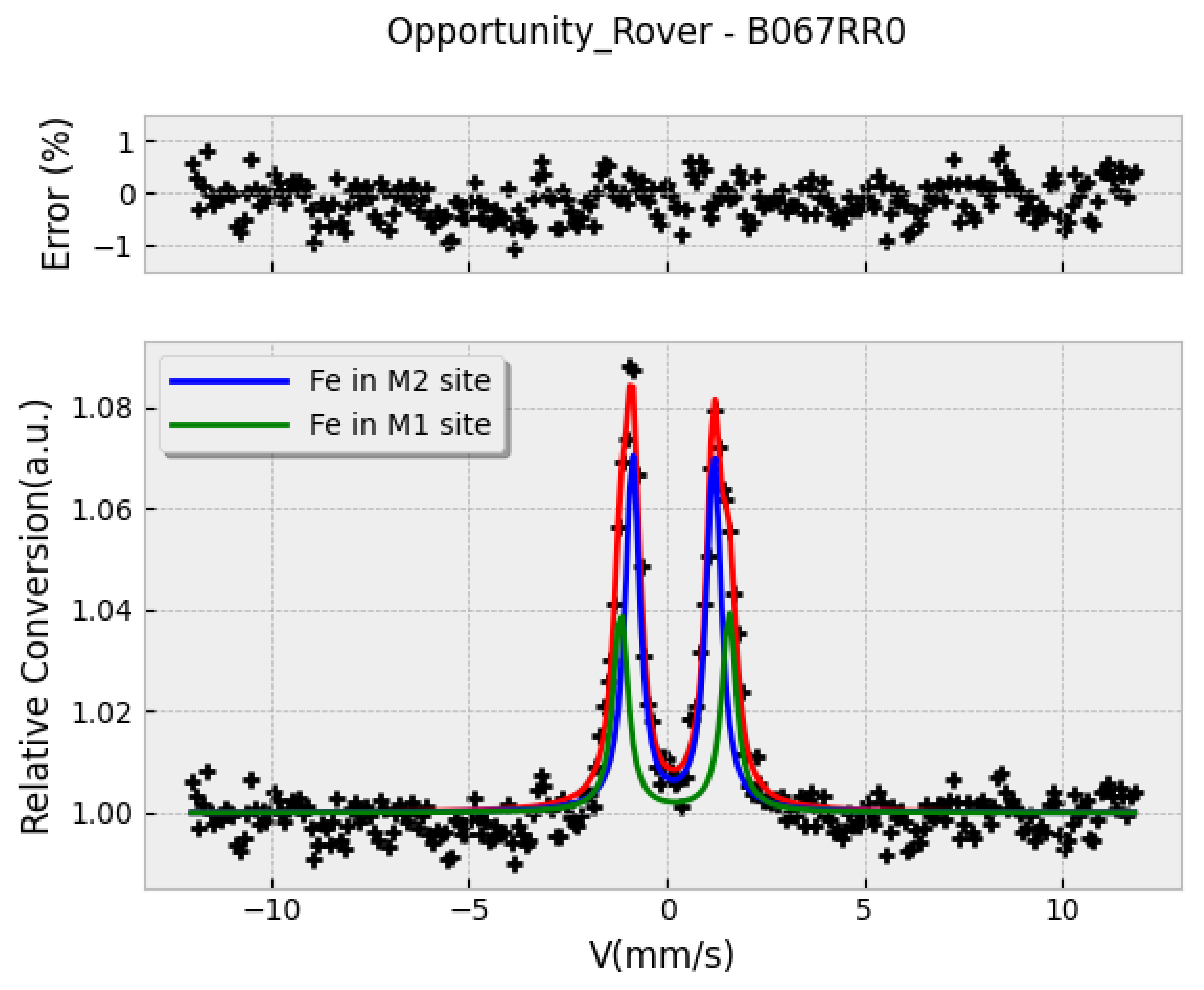
Figure 10.
57 Mössbauer spectra of an Iguazú falls soil sample (Argentina-Brazil border)
Disclaimer/Publisher’s Note: The statements, opinions and data contained in all publications are solely those of the individual author(s) and contributor(s) and not of MDPI and/or the editor(s). MDPI and/or the editor(s) disclaim responsibility for any injury to people or property resulting from any ideas, methods, instructions or products referred to in the content. |
© 2025 by the authors. Licensee MDPI, Basel, Switzerland. This article is an open access article distributed under the terms and conditions of the Creative Commons Attribution (CC BY) license (http://creativecommons.org/licenses/by/4.0/).
Copyright: This open access article is published under a Creative Commons CC BY 4.0 license, which permit the free download, distribution, and reuse, provided that the author and preprint are cited in any reuse.


