
Submitted:
25 June 2025
Posted:
26 June 2025
You are already at the latest version
Abstract
The paper explores cybersecurity risk modeling for Open Data in Smart City environments, with a specific case study focused on the Hradec Kralove Region. The goal is to establish a cybersecurity baseline through automated analysis using extended BPMN modeling, complemented by Business Impact Analysis (BIA). The approach identifies critical data flows and quantifies the impact of disruptions in terms of Recovery Time Objective (RTO), Maximum Tolerable Period of Disruption (MTPD), and Maximum Tolerable Data Loss (MTDL). A framework for automated risk mitigation selection is proposed. Results demonstrate the effectiveness of combining process mapping with security requirements to prioritize protections for smart city data. This structured methodology enhances data availability and integrity, supporting resilient urban digital infrastructure.
Keywords:
Smart City cybersecurity
; open data
; Business Impact Analysis (BIA)
; BPMN modeling
; risk mitigation
; data integrity
; RTO
; MTDL
1. Introduction
The proliferation of digital infrastructure, open data initiatives, and Internet of Things (IoT) technologies has fundamentally reshaped the design and operation of Smart Cities. These systems promise increased transparency, data-driven decision-making, and improved public services. However, this digital transformation also introduces a growing spectrum of cybersecurity threats. The security of open data platforms is critical: public sector systems process and expose datasets that may directly affect public safety, infrastructure management, or critical citizen services. Therefore, the design of secure-by-default architectures and risk-informed governance mechanisms is essential.
A significant challenge lies in the absence of tailored cybersecurity frameworks that consider both the interdependencies of Smart City processes, and the criticality of the data involved. Traditional information security standards such as ISO/IEC 27001 and NIST SP 800-53B [1] offer generic baselines but often lack operational granularity when applied to context-rich urban environments. Moreover, common vulnerability assessment practices fail to account for business continuity parameters like Recovery Time Objective (RTO), Maximum Tolerable Period of Disruption (MTPD), or Maximum Tolerable Data Loss (MTDL), which are vital for prioritizing mitigations in urban ecosystems.
In this context, Business Impact Analysis (BIA) provides a powerful but underutilized methodology for connecting cybersecurity decisions with real-world consequences. BIA is widely adopted in disaster recovery and business continuity planning, but its use in modeling cyber threats in Smart City environments is still emerging. Previous works have explored process-driven security modeling using Business Process Model and Notation (BPMN) [2], including security-focused extensions such as SecBPMN [3] or domain-specific models such as BPMN-SC [4]. However, these approaches rarely incorporate BIA metrics to quantify impact and prioritize controls based on measurable continuity criteria.
This study proposes an integrated methodology that extends BPMN-SC with embedded BIA metrics, applied to the real-world case of the Hradec Kralove Region Open Data Platform. Our goal is to build a cybersecurity baseline model that not only maps the functional flows of public service data but also supports automated derivation of mitigation measures based on service criticality. We introduce:
- A formalized model for capturing data availability, confidentiality, and integrity requirements within BPMN diagrams.
- A BIA-based annotation mechanism for process steps, assigning RTO, MTPD, and MTDL parameters to assess operational impact.
- An algorithmic approach to match risks with security controls, optimizing for coverage and efficiency.
- A practical evaluation of risk severity and mitigation through the automated publishing process of Smart City datasets.
The research builds upon national strategies and legislative frameworks, including the EU NIS2 Directive [5], ENISA’s baseline for IoT security [6], and recommendations from cybersecurity ontologies such as UCO [7] and CASE [8]. In contrast to previous static taxonomies, our approach emphasizes dynamic prioritization, allowing municipalities to align cyber defense with the operational relevance of data assets. The methodology contributes to the field by bridging process modeling, continuity management, and adaptive risk mitigation in the cybersecurity governance of Smart Cities.
The remainder of the paper is structured as follows. Chapter 2 reviews relevant literature in Smart City cybersecurity, with emphasis on security frameworks (e.g., ISO/IEC 27001, NIST SP 800-53B), process modeling (BPMN, BPMN-SC), and the limited but growing role of Business Impact Analysis (BIA). This forms the conceptual basis of the paper. Chapter 3 introduces the methodology that combines BPMN-SC with BIA metrics such as RTO, MTPD, and MTDL, allowing for risk-informed modeling of public service processes.
Chapter 4 presents an algorithm that prioritizes mitigation measures based on risk coverage efficiency. The approach aligns with the objectives of the ARTISEC project focused on AI-based cybersecurity planning. Chapter 5 applies the model to the Hradec Kralove Open Data Platform. The evaluation validates the ability of the approach to identify critical data flows and optimize protective measures. Chapter 6 summarizes key findings and discusses strategic and regulatory implications, including future potential for automation and AI-supported compliance under frameworks like NIS2. Key contributions of the paper include:
- A novel integration of Business Impact Analysis (BIA) with Smart City process modeling, allowing impact-oriented cybersecurity assessment through quantifiable metrics such as RTO, MTPD, and MTDL.
- A formal methodology for embedding BIA parameters directly into BPMN-SC diagrams, enabling process-aware prioritization of security controls based on service criticality and data classification.
- The development of a decision-support algorithm that selects mitigation measures based on risk coverage efficiency, optimizing the allocation of cybersecurity resources while fulfilling continuity requirements.
- A validation of the proposed framework in a real-world case study of the Hradec Kralove Region Open Data Platform, demonstrating its applicability in municipal public administration.
- Alignment of the proposed model with current and emerging regulatory standards, including ISO/IEC 27001, ISO 22301, and the EU NIS2 Directive, facilitating its adoption in compliance-driven environments.
- A contribution to the ARTISEC project by linking static process models with AI-ready structures for future automation in threat impact recalibration and risk-based security planning.
The proposed approach offers a replicable, regulation-aligned, and impact-driven framework which also provides a replicable foundation for municipal cybersecurity planning, supporting both the strategic vision and operational resilience of Open Data in Smart Cities.
2. Related Work
2.1. Cybersecurity in Smart Cities: From Technology to Process Awareness
Smart Cities are characterized by a convergence of technologies including IoT sensors, cloud/edge computing, big data analytics, and AI-driven decision support systems. This complexity introduces significant security risks. According to the Berkeley Center for Long-Term Cybersecurity (CLTC) [9], IoT and smart technologies pose higher systemic risks than other IT infrastructures due to their embedded nature and constant connectivity. Moreover, legacy systems and open data policies increase the attack surface [10]. ENISA [6] emphasizes the risks inherent in public data infrastructures and recommends contextual security assessments. Similarly, Kokolakis et al. [11] argue that a static perimeter-based view of security fails in smart environments and call for a process-aware model to capture the interdependence of city functions. Deloitte [12] highlights that resilience in Smart Cities requires collaboration between IT and OT domains, secure identity management, and a trust framework for data transactions.
Agrawal and Hubballi emphasize the technical implications of cyber-attacks on Smart Grid networks, highlighting their potential to disrupt critical infrastructure operations [13]. The NIS2 Directive [14] outlines specific obligations for key entities, including public administrations and digital infrastructure providers. These include mandatory risk analysis, BCP integration, and reporting thresholds for incidents. Although national implementations vary, the Directive sets a unifying European baseline.
2.2. BPMN and Data-Driven Security Analysis
The Business Process Model and Notation (BPMN) has been applied in various security contexts to capture workflows, roles, and data exchanges. Kokolakis et al. [15] and San Martín et al. [16] demonstrated how BPMN can be extended with risk and access control semantics to improve security modeling in complex systems. Salnitri et al. [17] introduced SecBPMN to embed high-level security goals into BPMN diagrams. Rodriguez et al. [18] focused on modeling security requirements using BPMN2.0 extensions. Building on these foundations, Horalek et al. [19] proposed BPMN-SC—an adaptation of BPMN tailored for Smart City domain modeling, mapping public functions, actors, and data flows. Our work extends this by integrating BIA metrics into BPMN-SC process elements, assigning Recovery Time Objective (RTO), Maximum Tolerable Period of Disruption (MTPD), and Maximum Tolerable Data Loss (MTDL) values. This enables visual prioritization of security requirements, bridging the gap between process modeling and business continuity planning.
2.3. Security Baselines and Standards: From Static Controls to Dynamic Risk Models
NIST’s SP 800-53B [1] and ISO/IEC 27001 [20] provide foundational security control baselines, while ENISA [6] recommends adapting these based on IoT-specific context. Our work extends these baselines by linking them to dynamic criteria from BPMN-based process analysis and recovery time objectives. This ensures alignment with the European Innovation Partnership on Smart Cities [21] and supports sector-specific adaptation.
2.4. Ontologies and AI Support for Smart City Cybersecurity
Ontology-based frameworks such as those from Mozzaquatro et al. [22], Syed [23], and UCO [12] aim to formalize and unify security models. However, they often lack real-time adaptability. Our work integrates BPMN-SC with BIA to enable adaptive threat prioritization. Temple et al. [8] and the ARTISEC project support AI-driven recalibration of BIA thresholds for evolving urban environments.
2.5. Comparative Analysis
The following table provides a structured comparison of our integrated BPMN-SC + BIA methodology with conventional and emerging approaches in cybersecurity modeling. It emphasizes that only our method supports simultaneous modeling of workflows, quantification of recovery thresholds, and specificity to Smart City operational structures. the relative positioning of our proposed BPMN-SC + BIA methodology against widely used approaches. We emphasize that only our model combines process mapping, quantified impact metrics, and smart city-specific functional modeling in a unified and traceable framework Table 1.
2.6. Impact-Driven Risk Modeling and BIA Integration
Although the architectural and systemic aspects of Smart City cybersecurity have been extensively addressed in the literature, one recurring limitation is the insufficient operationalization of these models. In particular, few works link cybersecurity prioritization with service continuity management in a measurable and process-specific manner.
Business Impact Analysis (BIA), a methodology well-established in business continuity planning [16], introduces measurable thresholds for acceptable service disruptions: Recovery Time Objective (RTO), Maximum Tolerable Period of Disruption (MTPD), and Maximum Tolerable Data Loss (MTDL). These metrics enable organizations to define the operational importance of business processes and data assets. Despite its usefulness, BIA has been underutilized in cybersecurity-specific research within Smart City environments. The combination of BIA with business process modeling, specifically BPMN extended to Smart City contexts (BPMN-SC), represents a methodological advancement. Sobeslav et al. [19] demonstrated how BPMN-SC can capture domain-specific functional flows across municipal services. Building upon this, our approach embeds BIA parameters within these process flows, aligning asset protection with continuity thresholds.
This integration supports the simulation of cascading failures and enables pre-emptive identification of high-risk processes and datasets. By incorporating BIA directly into BPMN-SC nodes, we create a framework that informs cybersecurity strategy with quantified disruption tolerance. This responds to calls by ENISA [6] and NIS2 [14] for dynamic risk assessment methodologies aligned with organizational impact.
Comparable works by Salnitri et al. [17] and San Martín et al. [16] also explored linking business process security requirements with model-driven engineering. However, these often lack impact metrics grounded in service continuity, which are essential for prioritization under constrained resource scenarios. Similarly, ontology-based approaches like those of Mozzaquatro et al. [22] and Syed [23,24] offer semantic rigor but do not translate directly into operational timelines for recovery and mitigation.
In contrast, our method enables Smart City stakeholders, particularly municipal IT managers and data governance authorities, to align cyber defense priorities with BIA thresholds, ensuring that the most critical data streams (e.g., emergency services, environmental sensors, eGovernment platforms) are protected to the degree their function necessitates. Moreover, this aligns with ISO/IEC 27001 Annex A.17, which mandates information security aspects of business continuity management.
Looking ahead, several promising directions emerge:
- AI-enhanced BIA recalibration: As proposed in the ARTISEC project, AI tools can dynamically adjust RTO and MTPD values based on usage telemetry or threat landscape shifts.
- Domain-specific BIA catalogs: Extending the framework for sectoral adaptation (e.g., transportation, utilities, health services) in line with domain risk registers, such as those defined in NIST SP 800-30 and ISO 31010.
- Compliance automation: Integrating this model into automated audit frameworks, enabling traceable justification of control selection during regulatory inspections.
The synergistic use of BIA, BPMN-SC, and regulatory alignment introduces a robust mechanism to prioritize cybersecurity efforts not based on abstract threat scenarios, but on real-world, quantified consequences of disruption. This represents a critical shift in how cyber risk is modeled, communicated, and acted upon in the governance of data-centric Smart City systems.
3. Business Impact Analysis Methodology
This chapter outlines a methodology that integrates Business Impact Analysis (BIA) with BPMN-SC to assess cybersecurity risks and service continuity parameters within Smart City systems [25]. The goal is to enable data-driven prioritization of security measures by embedding quantitative indicators into process models [26,27].
3.1. Establishing Impact Criteria
The first step is to define a set of impact criteria that reflect the severity of disruptions from the perspective of financial costs, reputational damage, and personal safety risks. These criteria are aligned with recommendations under the EU NIS2 Directive and reflect national best practices for critical infrastructure protection [28,29]. Impact levels are categorized to guide both risk assessment and the selection of proportionate safeguards Table 2.
3.2. Availability as a Key Parameter
The first evaluation criterion is availability. Availability is defined as ensuring that information is accessible to authorized users at the moment it is needed. In some cases, the destruction of certain data may be viewed as a disruption of availability. It is therefore essential to clarify what vendors mean when they state that their system guarantees, for example, 99.999% availability. If the base time period is defined as 365 days per year, this figure allows for a maximum unavailability of about 5 minutes annually [30,31].
At first glance, five-nines availability seems sufficient. However, it is important to define what exactly is meant by “system.” Vendors often refer only to the hardware layer, omitting operating systems and applications. These layers are frequently excluded from SLAs and come with no guaranteed availability, even though in practice, they are often the cause of outages Table 3.
Even though annual percentage availability is widely used, it is far more precise and practical to define:
- Recovery Time Objective (RTO): the maximum tolerable duration of service downtime.
- Recovery Point Objective (RPO): the maximum tolerable amount of data loss.
If RTO = 0, this implies fully redundant infrastructure. RTO defines how quickly operations must resume, and is central to disaster recovery planning. RPO defines the volume of data loss an organization is willing to accept. Together, RTO and RPO form the foundation of continuity planning.
Additional availability-related parameters include:
- MIPD (Maximum Initial Programmed Delay): the maximum allowed time to initialize and start a process after a failure.
- MTPD (Maximum Tolerable Period of Disruption): the maximum downtime allowed before the disruption causes unacceptable consequences for operations.
- MTDL (Maximum Tolerable Data Loss): the maximum data loss acceptable before critical impact occurs.
When high availability is required, duplication of all system components (power, disks, servers, etc.) is a logical solution. However, duplicating multi-layer architectures increases system complexity and the risk of failure (e.g., zero-day vulnerabilities or failover misconfigurations).
If each component guarantees 99.999% availability, the availability of the entire system, when modeled as three interdependent layers, is approximately 99.997%, which equates to about 16 minutes of allowable downtime per year. Such configurations must also handle failover, active/passive role switching, and user redirection without compromising data integrity. Otherwise, “split-brain” scenarios may occur, where independent operation of redundant components leads to data divergence and inconsistency.
To support BIA, impact evaluations must assess downtime in intervals of 15 minutes, 1 hour, 1 day, and 1 week. The following availability categories apply:
- C: Low importance—downtime of up to 1 week is acceptable.
- B: Medium importance—downtime should not exceed one business day.
- A: High importance—downtime of several hours is tolerable but must be resolved promptly.
- A+: Critical—any unavailability causes serious harm and must be prevented.
These assessments help derive:
- MIPD: Based on severity across time intervals using logic functions (e.g., if 15min = B/A/A+, then MIPD = 15min).
- MTPD: Longest acceptable time without recovery.
- MTDL: Largest data volume/time tolerable for loss.
Example of MIPD determination:
- If unavailability at 15min = B/A/A+ → MIPD = 15 min.
- Else if 1hr = B/A/A+ → MIPD = 1 h.
- Else if 1 day = B/A/A+ → MIPD = 1 day.
- Else if 1 week = B/A/A+ → MIPD = 1 week.
- Else → MIPD = “BE” (beyond acceptable threshold).
These values ensure the architecture design meets operational expectations for continuity and resilience. Rather than relying solely on annual percentage availability, this methodology emphasizes two well-defined parameters:
- Recovery Time Objective (RTO): Maximum acceptable time to restore service after disruption.
- Recovery Point Objective (RPO): Maximum acceptable data loss measured in time prior to an incident.
Both RTO and RPO are critical inputs to continuity planning and are directly linked to the architectural design of backup, redundancy, and failover mechanisms.
3.3. Confidentiality and Integrity Considerations
Another essential parameter evaluated in this methodology is confidentiality. Confidentiality is commonly defined as ensuring that information is only accessible to those who are authorized to view it. In cybersecurity, unauthorized access or disclosure of data is considered a breach of confidentiality. To address this, organizations should implement appropriate classification schemes and technical, organizational, and physical security measures [32].
The commonly used classification scheme includes:
- Public: Information intended for general public access.
- Internal: Information accessible only to internal employees.
- Confidential: Information restricted to selected employees.
- Strictly Confidential: Highly sensitive information accessible only to designated personnel.
The classification level may change during the information lifecycle. To maintain confidentiality, proper controls should be in place for data access, encryption, and logging.
Integrity ensures the correctness and completeness of information. Any unauthorized or accidental modification—whether due to error, attack, or system failure—can violate data integrity. The risk is especially high if such modifications remain undetected for long periods.
To ensure data integrity, the following techniques can be applied:
- Cryptographic Hash Functions (e.g., SHA-256): Used to verify whether data has changed.
- Digital Signatures: Validate the authenticity and integrity of documents using asymmetric cryptography.
- Checksums: Simple integrity-check algorithms.
- Message Authentication Codes (MAC): Combine a secret key with data to generate verifiable integrity tags.
- Digital Certificates: Verify sender authenticity and data integrity via trusted certificate authorities.
A best practice includes logging all data changes and implementing layered encryption—e.g., encrypting data at the application level before storage, and using checksum validation upon retrieval. While this shifts risk from the database to the application, it enables protection even against insider threats when managed through HSM (Hardware Security Module) devices.
3.4. Example of Security Baseline Application
The implementation of the security baseline for open data in the Hradec Kralove Region, including the automated selection of security measures, is demonstrated in the process of data publication and visualization through the regional open data portal.
The process starts with a request to publish a chart or map visualization. The request, containing a visualization URL, is received from a user or administrator. The system then processes the request and provides the appropriate URL. The visualization is embedded into an e-frame on the portal and properly configured.
Following this, the visualization is published. A display check is performed to verify correct rendering. If the visualization fails to display, a corrective action loop is triggered (“Display Fix Loop”), after which the publishing attempt is repeated.
Once the visualization passes the check, it is made available to the public. End users can then view the newly published charts and maps through the open data portal interface.
This example demonstrates how BIA metrics and process modeling can be used not only for threat analysis but also for enhancing the resilience of real-world Smart City services. To operationalize BIA in Smart City contexts, this study embeds RTO/RPO/MTDL thresholds directly into BPMN-SC diagrams. Each process task or data flow is annotated with impact parameters. This enables simulation of cascading failures and evaluation of interdependencies among services (e.g., how a disruption in environmental data publishing affects public health dashboards).
Additionally, the model includes:
- Maximum Tolerable Period of Disruption (MTPD): Time beyond which continued disruption is unacceptable.
- Maximum Tolerable Data Loss (MTDL): Volume or timeframe of acceptable data loss based on legal and operational factors.
This step establishes a machine-readable baseline for impact, which can be further linked to automated risk assessment and mitigation tools as outlined in the next chapter.
The result is a context-sensitive, standardized input layer for cybersecurity planning that reflects actual service delivery constraints, not just abstract technical vulnerabilities Table 4.
Figure 1.
BPMN_SC model.
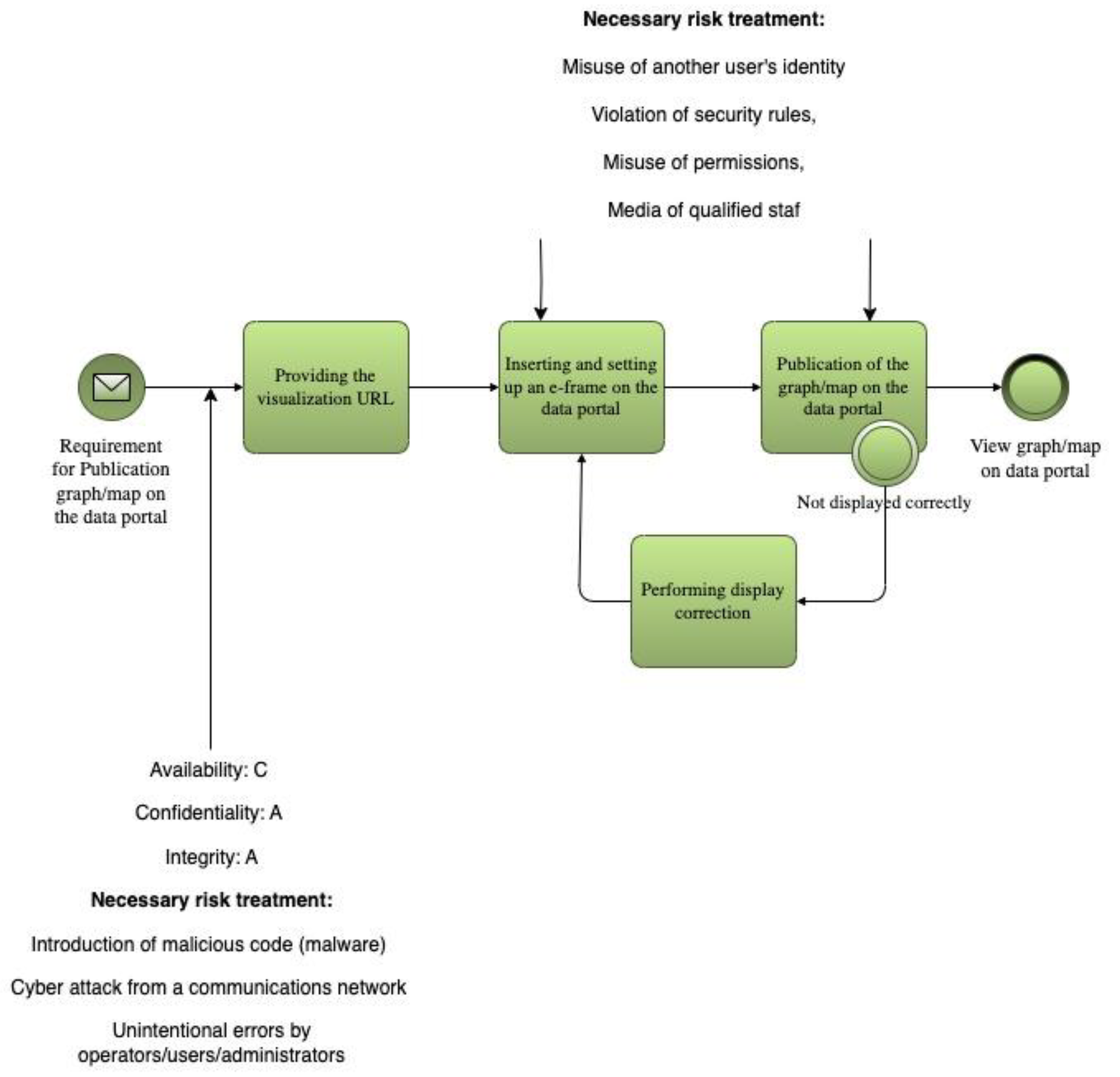
The risk posture of the system is significantly influenced by the level of integrity and confidentiality assigned to data prior to publication. These two dimensions are critical to ensuring the relevance and trustworthiness of the open data portal’s Operations Table 5.
Key cybersecurity risks that must be addressed, based on this risk analysis, include:
- Identity theft
- Security breaches or misuse of credentials/media
- Cyber-attacks via communication networks
- Operator or administrator errors
- Lack of qualified personnel
These risks primarily affect the staff involved in the creation, publication, and visualization of data sets, including both system administrators and data processors. The recommended mitigation measures reflect the need for:
- Identity and access management
- Malware detection and prevention
- Continuous staff training and awareness
4. Automated Selection of Risk-Mitigation Measures from Security Baseline
4.1. The Greeddy Alghorithm for Automated Selection of Risk-Mitigation
The task is to select the best measure (rows of the table) to address the given risks (columns of the table). We have a table of measures with rows M and columns representing defined risks R. Each row of M mitigates only some of the risks R. Given a set of measures SM, the task is to select from SM the rows that cover the maximum number of defined risks R, considering the effectiveness of each measure E.
Definitions:
- Set of measures (rows), where M is the total number of measures —
- Set of risks (columns), where R is the total number of risks —
- A subset of measures from which we are selecting -
- — a binary value indicating whether measure covers risk (if it does, ; otherwise ).
- — efficiency of measure , where 1 is the least efficient and 5 is the most efficient.
- — decision variable, where indicates that measure is selected, and indicates that it is not selected.
Objective function — maximizing risk coverage with respect to efficiency:
This formula states that each risk is assigned a value of 1 if it is mitigated by at least one measure, with measures with a higher having a higher weight.
Constraints — ensuring that measures are selected only from the SM set:
This constraint says that the selection of measures is limited to the set (a subset of all measures).
Risk coverage - ensuring that the risk is covered:
This constraint ensures that each risk is covered by at least one selected measure.
Goal of the Algorithm:
The goal is to find a subset of measures that maximizes coverage of risks R, considering their efficiency.
Mathematical Procedure:
-
Initialization:
- ○
- Define the set of uncovered risks .
- Initialize an empty set of selected measures .
- 2.
-
Scoring Each Measure:
- ○
- For each measure , compute its score:
Where:
- “
- a higher priority if more risks are covered).
Iterative Measure Selection:
Repeat the following steps until all risks are covered or no more measures can be selected:
- risks are covered, the algorithm terminates.
Output:
The set of selected measures S, which maximizes the number of covered risks considering the efficiency.
- Therefore, if the objective is to maximize overall risk coverage, taking into account the effectiveness of each selected measure, we can assume that these constraints are met:
- Each measure can only cover some of the risks represented by the matrix.
-
The selection of measures must maximize the coverage of all risks R, with preference given to measures with a higher efficiency score .Formulate the mathematics problem as follows:Where:
- determines whether a measure addresses a risk .
- is the decision variable for selecting the measure.
- weights the selection based on the efficiency of the measure, with higher efficiency receiving a lower penalty.
The goal is to select measures that cover the maximum number of risks with the highest possible efficiency.
Example:
Consider 3 measures and 5 risks. The coverage matrix and efficiency are defined as follows:
-
Compute the score for each measure:
- ○
- : 3 risks covered, efficiency 5 → score
- ○
- : 3 risks covered, efficiency 3 → score
- ○
- : 3 risks covered, efficiency 4 → score
- Select , since it has the highest score (1.0).
- Update the set of uncovered risks. covers risks .
- Recompute scores for remaining measures and (adjust for the updated set of uncovered risks).
- Continue iterating until all risks are covered or no further improvement is possible.
4.2. Advantages and Disadvantages of Using the Greedy Algorithm
The following sub-chapter discusses the Advantages and disadvantages of using the Greedy algorithm for a model with 40 measures and 14 risks. The measures were focused mainly on speed, simplicity, efficiency and other important factors.
Advantages:
-
Speed: The Greedy algorithm is fast because it makes locally optimal choices at each step. With 40 measures and 14 risks, the algorithm should perform efficiently.
- ○
- The time complexity is roughly , where mmm is the number of measures and nnn is the number of risks. For and , this is computationally manageable.
- Simplicity: The algorithm is easy to implement and does not require complex setups or specialized optimization libraries. It can be realized in any programming language.
- Approximation: Greedy algorithms often provide solutions that are close to optimal, especially when there are no significant overlaps in risk coverage between the measures.
- Consideration of Efficiency: The algorithm accounts for the efficiency of measures, which is beneficial when measures have significantly different efficiencies.
Disadvantages:
-
Local Optimality: The Greedy algorithm focuses on making the best choice at each step, which can lead to suboptimal solutions. If measures have large overlaps in risk coverage, the Greedy algorithm might select solutions that are not globally optimal.
- ○
- It may choose a measure that covers many risks in the short term, but in later steps, more efficient measures might be ignored.
- Inability to Consider Dependencies: If there are dependencies between measures or if certain measures have different priorities, the Greedy algorithm cannot effectively account for them. This may result in a less effective overall solution.
- Sensitivity to Efficiency Distribution: If the efficiencies of the measures are too closely distributed, the Greedy algorithm might fail to find a sufficiently optimal solution. Small differences in efficiency may cause the algorithm to overlook measures that would be more beneficial in the long run.
A suitable proof of the efficiency and correctness of the above relations and methods can be made by formal argumentation. A structured approach to proving the correctness of the generalized formula and method is presented here:
Theoretical Proof (Formal Reasoning)
Objective Function:
We aim to maximize risk coverage while considering the efficiency of each measure. The objective function is:
- Risk Coverage: Each represents whether a measure addresses a risk . Summing over all jjj allows us to count how many risks are covered by measure .
- Efficiency Weighting: Each term is divided by , which penalizes measures with lower efficiency. Higher efficiency (lower ) contributes more favorably to the objective function.
Therefore, the objective function maximizes the total number of risks covered, weighted by the efficiency of the measures. Selecting a measure with higher efficiency () will lead to a lower penalty , promoting efficient measures.
Selection Criteria
The decision variable ensures that we only select a measure if it is part of the solution. The sum of over all jjj correctly counts the number of risks covered by the selected measures. The theoretical model thereby correctly represents the goal of covering the maximum number of risks with the highest possible efficiency.
Greedy Algorithm Proof
The Greedy algorithm described in earlier sections makes locally optimal choices at each step by selecting the measure with the best coverage-to-efficiency ratio.
Step 1: Greedy Choice Property
Greedy algorithms work when the greedy choice property holds, i.e., making a local optimal choice at each step leads to a globally optimal solution.
In this case, each step selects the measure that maximizes:
This ratio ensures that at each step, the algorithm picks the measure that offers the greatest coverage of uncovered risks per unit of efficiency. Although Greedy algorithms do not always guarantee a globally optimal solution for all types of optimization problems, for risk coverage problems with efficiency weighting, this method often produces solutions that are close to optimal.
Step 2: Greedy Algorithm Approximation Bound
For problems like weighted set cover, where we aim to cover a set of elements (in this case, risks) with a minimal weighted set of subsets (in this case, measures with efficiency weighting), it is known that a Greedy algorithm provides an approximation within a logarithmic factor of the optimal solution. The Greedy algorithm provides a logarithmic approximation bound for set cover problems:
Where is the harmonic number, and nnn is the number of elements to be covered (in this case, the number of risks).
Therefore, while the Greedy algorithm may not always provide the exact optimal solution, it is guaranteed to be within a factor of of the optimal solution, making it a good heuristic for problems like this.
5. Discussion and Results
A theoretical proof is accompanied by empirical validation, where we test the algorithm on a real or simulated dataset to demonstrate that the relationships and methods function correctly in practice.
Example Simulation:
We can simulate a problem with 40 measures and 14 risks. Each measure has a random efficiency score between 1 and 5, and the coverage matrix is randomly generated. We run the Greedy algorithm and compare it to a brute-force optimal solution or known benchmarks for validation.
Simulation Steps:
- 4.
- Generate a random coverage matrix , where each element is 0 or 1.
- 5.
- Assign efficiency values randomly to each measure from the set .
- 6.
- Run the Greedy algorithm to select measures that maximize coverage while considering efficiency.
- 7.
- Compare results with brute-force selection (optimal solution for small instances) or other optimization algorithms (like integer linear programming).
Expected Outcome:
The Greedy algorithm should select measures that cover most risks while minimizing the efficiency penalty.
- For small instances (e.g., 10 measures and 5 risks), we can compute the optimal solution via brute force and compare it to the Greedy result. The Greedy solution should be close to optimal.
- For larger instances (e.g., 40 measures and 14 risks), Greedy will efficiently find a near-optimal solution in a fraction of the time it would take to compute the exact solution.
Conclusion from Empirical Testing:
The empirical testing demonstrates that the proposed Greedy algorithm and formula function correctly, providing solutions that cover a high number of risks efficiently. The approximation quality will be close to the theoretical guarantees.
Empirically verify
To empirically verify the use of the genetic algorithm (GA) for selecting optimal risk coverage measures and its comparison with the Greedy algorithm, a Python test was designed and implemented. This test involved generating random data for 14 risks and 40 measures, implementing both algorithms and evaluating their performance. The following metrics were validated and used for comparison.
- Coverage: number of risks covered.
- Effectiveness: sum of the effectiveness scores of the selected measures.
- Number of measures selected: Total number of measures selected.
- Execution time: The time required to run each algorithm.
import numpy as np
import random
import time
from functools import reduce
# Seed for reproducibility
np.random.seed(42)
# Number of risks and measures
num_measures = 40
num_risks = 14
# Generate random coverage matrix (40x14) and effectiveness vector (1-5)
coverage_matrix = np.random.choice([0, 1], size=(num_measures, num_risks), p=[0.7, 0.3])
effectiveness = np.random.randint(1, 6, size=num_measures)
# Helper function to calculate fitness
def fitness(individual):
covered_risks = reduce(np.logical_or, [coverage_matrix[i] for i in range(num_measures) if individual[i] == 1], np.zeros(num_risks))
covered_risks_count = np.sum(covered_risks)
total_efficiency = sum([effectiveness[i] for i in range(num_measures) if individual[i] == 1])
return covered_risks_count, total_efficiency
# Genetic Algorithm (GA)
def genetic_algorithm(population_size=100, generations=200, mutation_rate=0.1):
# Initialize random population
population = [np.random.choice([0, 1], size=num_measures) for _ in range(population_size)]
best_individual = None
best_fitness = (0, 0)
for generation in range(generations):
# Evaluate fitness of each individual
fitness_scores = [fitness(individual) for individual in population]
# Select the best individual
for i, f in enumerate(fitness_scores):
if f > best_fitness:
best_fitness = f
best_individual = population[i]
# Selection (roulette wheel selection based on fitness)
total_fitness = sum(f [0] for f in fitness_scores)
selected_population = []
for _ in range(population_size):
pick = random.uniform(0, total_fitness)
current = 0
for i, f in enumerate(fitness_scores):
current += f [0]
if current > pick:
selected_population.append(population[i])
break
# Crossover (single-point crossover)
new_population = []
for i in range(0, population_size, 2):
parent1, parent2 = selected_population[i], selected_population[i+1]
crossover_point = random.randint(0, num_measures-1)
child1 = np.concatenate((parent1[:crossover_point], parent2[crossover_point:]))
child2 = np.concatenate((parent2[:crossover_point], parent1[crossover_point:]))
new_population.extend([child1, child2])
# Mutation
for individual in new_population:
if random.random() < mutation_rate:
mutation_point = random.randint(0, num_measures-1)
individual[mutation_point] = 1 - individual[mutation_point] # Flip bit
population = new_population
return best_individual, best_fitness
# Greedy Algorithm
def greedy_algorithm():
selected_measures = []
remaining_risks = np.zeros(num_risks)
while np.sum(remaining_risks) < num_risks:
best_measure = None
best_coverage = -1
best_efficiency = -1
for i in range(num_measures):
if i in selected_measures:
continue
measure_coverage = np.sum(np.logical_and(coverage_matrix[i], np.logical_not(remaining_risks)))
if measure_coverage > best_coverage or (measure_coverage == best_coverage and effectiveness[i] > best_efficiency):
best_measure = i
best_coverage = measure_coverage
best_efficiency = effectiveness[i]
if best_measure is None:
break
selected_measures.append(best_measure)
remaining_risks = np.logical_or(remaining_risks, coverage_matrix[best_measure])
total_efficiency = sum(effectiveness[i] for i in selected_measures)
return selected_measures, len(selected_measures), total_efficiency
# Run tests and compare
# Genetic Algorithm
start_time = time.time()
best_solution_ga, best_fitness_ga = genetic_algorithm()
time_ga = time.time() - start_time
# Greedy Algorithm
start_time = time.time()
selected_measures_greedy, num_selected_greedy, efficiency_greedy = greedy_algorithm()
time_greedy = time.time() - start_time
# Results
print(“Genetic Algorithm:”)
print(f”Best solution (GA) covers {best_fitness_ga [0} risks with total efficiency {best_fitness_ga [1]}”)
print(f”Time taken: {time_ga:.4f} seconds”)
print(“\nGreedy Algorithm:”)
print(f”Selected measures (Greedy) covers {num_risks} risks with total efficiency {efficiency_greedy}”)
print(f”Number of selected measures: {num_selected_greedy}”)
print(f”Time taken: {time_greedy:.4f} seconds”)
Implementation of genetic algorithm:
Initialize a random population of solutions. Fitness is calculated based on how many risks are covered and what the overall efficiency is. Selection is done by roulette wheel, crossover is single point and mutation shuffles random bits. The best solution is returned after a fixed number of generations. Genetic algorithm: It is expected to produce a near-optimal solution with a balance between risk coverage and efficiency measures, but may take longer.
An implementation of the Greedy algorithm:
Measures are selected based on how many uncovered risks they mitigate and their effectiveness. This process continues until all risks are covered or until no new measures can improve the solution. Greedy algorithm: It is expected to be faster, but may not find the best solution due to its greedy nature (locally optimal, but not globally optimal), Table 6.
The empirical validation of the proposed methodology demonstrates its effectiveness for risk-based control selection in the context of Smart City cybersecurity. Simulated experiments using 40 candidate mitigation measures and 14 predefined risk scenarios allowed for performance benchmarking of two algorithmic strategies: a Greedy algorithm and a Genetic Algorithm (GA).
The Greedy approach, optimized for speed and simplicity, consistently produced near-optimal results with minimal computation time, making it well-suited for operational deployments and real-time decision-making. Conversely, the Genetic Algorithm exhibited slightly higher overall risk coverage and better balancing of control effectiveness, but required significantly more computational resources. Therefore, it appears more applicable for strategic scenario planning and simulation environments.
Key evaluation metrics, such as risk coverage, aggregate effectiveness, number of measures selected, and execution time, confirm the theoretical expectations. The Greedy algorithm, while locally optimal, aligns with logarithmic approximation bounds known for weighted set-cover problems. The GA-based method, albeit more computationally intensive, delivers a marginal improvement in solution quality and robustness.
Importantly, the integration of Business Impact Analysis (BIA) into process modeling via BPMN-SC enables impact-aware prioritization. This ensures alignment with continuity thresholds (RTO, MTPD, MTDL) and provides a clear rationale for selecting specific security measures based on their business-criticality. Unlike static baseline approaches (e.g., ISO/IEC 27001 Annex A or NIST SP 800-53B), this model dynamically maps protections to service-level needs and operational constraints.
The findings further support the utility of the ARTISEC project’s direction, namely the future use of AI-driven recalibration of BIA metrics based on telemetry data and evolving threat landscapes. This demonstrates that algorithmic selection of controls can be grounded not only in risk coverage efficiency, but also in measurable continuity and availability targets.
6. Conclusions
This study responded to the growing demand for systematic and measurable cybersecurity planning in Smart City environments, with a focus on the often-overlooked domain of open data. By integrating Business Impact Analysis (BIA) with process modeling via BPMN-SC, the research introduced a replicable framework that allows municipalities to quantify disruption tolerances and align security measures with service continuity objectives.
The proposed methodology was systematically developed across six chapters. Chapter 2 synthesized existing literature and standards, identifying key limitations in static baseline approaches. Chapter 3 defined impact criteria and formalized the BIA annotation of Smart City processes. Chapter 4 presented an algorithm for the optimized selection of security controls based on risk coverage and measure efficiency. Chapter 5 empirically validated this algorithmic approach using simulated data for 40 measures and 14 risks, comparing a Greedy heuristic and a Genetic Algorithm to assess trade-offs between speed and optimality.
As part of the ARTISEC project, the methodology was applied to the Open Data Platform of the Hradec Kralove Region. Key publication processes were modeled using BPMN-SC, enriched with RTO, MTPD, and MTDL metrics. These enriched diagrams enabled the automated mapping of cyber risks to relevant mitigation controls drawn from a structured baseline catalogue.
This implementation provides tangible proof that cybersecurity planning can evolve beyond compliance to become data-driven, transparent, and aligned with the real operational demands of Smart City systems. The approach supports NIS2 Directive implementation and advances ISO/IEC 27001-aligned continuity strategies.
Future research should focus on expanding the automation potential of this framework, particularly by incorporating AI-driven adjustments to BIA parameters based on live telemetry and threat intelligence. Additional work is also warranted in extending the baseline catalogue to other public sector domains such as healthcare, transportation, or utilities, and in modeling interdependencies among controls.
Overall, the study lays a solid foundation for municipalities and infrastructure operators to strengthen cybersecurity governance through process-integrated, impact-sensitive, and algorithmically supported decision-making.
Funding
This work and paper were supported by the project “Application of Artificial Intelligence for En-suring Cyber Security in Smart City”, n. VJ02010016, provided by the Ministry of the Interior of the Czech Republic.
Data Availability Statement
Data sharing is not applicable.
Acknowledgments
This work and article were created in cooperation with the Hradec Králové Region, the application guarantor of the ARTISEC project. We would like to thank the regional government and all involved staff for their support.
Conflicts of Interest
The author declares no conflict of interest.
Appendix A

Table A1.
Risk table.
| Risks | ||
|---|---|---|
| Order no. | Title | Code |
| 1 | Misuse of another user’s identity | R01 |
| 2 | Violation of security rules, misuse of permissions, media. | R02 |
| 3 | Cyber-attack from a communication network | R03 |
| 4 | Introduction of malicious code (malware) | R04 |
| 5 | Technical or software malfunction | R05 |
| 6 | Failure/outage of support services (electricity, air conditioning,...) | R06 |
| 7 | Communication network failure/outage | R07 |
| 8 | Unintentional operator/user/administrator errors | R08 |
| 9 | Natural disasters | R09 |
| 10 | Lack of employees with the necessary qualifications | R10 |
| 11 | Violation of physical security, theft, vandalism, sabotage,... | R11 |
| 12 | Access to all data at the server and infrastructure level | R12 |
| 13 | Control over the content of processed data at the level of server solutions and infrastructure | R13 |
| 14 | Denial of service at the server and infrastructure level | R14 |
Table A2.
Mapping of measures for risks.
| Catalogue of measures | Risks | ||||||||||||||
|---|---|---|---|---|---|---|---|---|---|---|---|---|---|---|---|
| Order no. | Name of the measure | R01 | R02 | R03 | R04 | R05 | R06 | R07 | R08 | R09 | R10 | R11 | R12 | R13 | R14 |
| O1 | Ensuring the segmentation of the communication network | x | x | ||||||||||||
| O2 | Ensuring communication management within the communication network and the perimeter of the communication network | x | x | x | x | x | |||||||||
| O3 | Implementation of cryptography to ensure data confidentiality and integrity when accessing, managing or accessing a communication network remotely using wireless technologies | x | x | x | x | x | |||||||||
| O4 | Deploy a tool to actively block unwanted communication | x | x | ||||||||||||
| O5 | Deploy a tool to ensure the integrity of the communications network | x | x | ||||||||||||
| O6 | Implementation of a tool for managing and verifying the identity of users, administrators and applications | x | x | x | x | x | |||||||||
| O7 | Use of multi-factor authentication with at least two different types of factors | x | x | x | x | x | |||||||||
| O8 | Use of identity verification for users, administrators and applications that uses an account identifier and password for authentication, enforces 12 characters for users and 17 characters for administrators, and enforces mandatory password changes at intervals of no more than 18 months | x | x | x | x | x | |||||||||
| O9 | Deployment of a centralized tool for managing access permissions to individual ICT system assets and for reading data, writing data and changing permissions | x | x | x | x | x | |||||||||
| O10 | Deploying a malicious code protection tool | x | |||||||||||||
| O11 | Deployment of a tool to monitor and manage the use of removable devices and data carriers | x | |||||||||||||
| O12 | Deploying a tool to control permissions to run code | x | x | ||||||||||||
| O13 | Deploying a tool to control the automatic launch of removable device and data media content | x | |||||||||||||
| O14 | Deployment of a tool to record security and operational events of critical ICT assets | x | x | x | |||||||||||
| O15 | Deployment of a tool to synchronize the uniform time of technical assets at least once every 24 hours | x | |||||||||||||
| O16 | Deploying a cyber security event detection tool | x | x | x | |||||||||||
| O17 | Deployment of a tool for authentication and control of transmitted data within and between communication networks | x | x | x | |||||||||||
| O18 | Deployment of a tool for authentication and control of transmitted data on the perimeter of the communication network | x | x | x | |||||||||||
| O19 | Deploy a tool to block unwanted communication | x | |||||||||||||
| O20 | Deploy an application security tool to permanently protect applications, information and transactions from unauthorized activity and denial of service | x | |||||||||||||
| O21 | Deployment of currently resilient cryptographic algorithms and cryptographic keys to protect information and communication system assets | x | x | x | x | x | |||||||||
| O22 | Deploy a tool for using a key and certificate management system | x | x | x | |||||||||||
| O23 | Deploying a tool to use technical and software resources that are designed for a specific environment | x | |||||||||||||
| O24 | Ensuring restrictions on physical access to industrial, control systems and communication network | x | x | ||||||||||||
| O25 | Separation of the communication network dedicated to these systems from other infrastructure | x | x | ||||||||||||
| O26 | Deploy a tool to restrict and control remote access to these systems | x | |||||||||||||
| O27 | Regular monitoring of the supplier’s compliance with safety requirements | x | x | ||||||||||||
| O28 | Preparation and implementation of security policy compliance checks | x | x | x | |||||||||||
| O29 | Update of the Security Awareness Development Plan | x | x | x | |||||||||||
| O30 | Ensuring regular training and verification of employee safety awareness | x | x | x | |||||||||||
| O31 | Ensuring regular training and verification of security awareness of the supplier’s employees | x | x | ||||||||||||
| O32 | Ensuring evaluation of the effectiveness of the security awareness plan and the training provided | x | x | x | |||||||||||
| O33 | Determination of rules and procedures for dealing with violations of established security rules by users, administrators and persons in security roles | x | x | ||||||||||||
| O34 | Introduction of appropriate organizational measures | x | x | x | x | ||||||||||
| O35 | Installing and ensuring regular maintenance of the UPS | x | x | x | |||||||||||
| O36 | Installation and regular maintenance of the diesel generator | x | x | x | |||||||||||
| O37 | Regular checking of access permissions | x | x | x | x | x | |||||||||
| O38 | Regular checking of user accounts and their rights | x | x | x | |||||||||||
| O39 | Update of asset range | x | x | ||||||||||||
| O40 | Ensuring the retention period of event records for VIS and KII | X | X | x | |||||||||||
| O41 | Conducting penetration tests before assets are put into operation | x | x | x | x | ||||||||||
| O42 | Penetration testing in connection with a significant change | x | x | x | x | ||||||||||
| O43 | Ensuring system recovery after a cybersecurity incident. | x | x | x | x | x | x | ||||||||
| O44 | Checking the use and expiry of licenses | x | |||||||||||||
| O45 | Keeping records of major suppliers | x | |||||||||||||
| O46 | Informing major suppliers of their records | x | |||||||||||||
| O47 | Supplier risk management | x | |||||||||||||
| O48 | Establishing rules and procedures to protect against malicious code | x | |||||||||||||
| O49 | Limiting and controlling the use of software resources | x | x | x | |||||||||||
| O50 | Limiting and controlling the supply chain | x | x | x | |||||||||||
References
- National Institute of Standards and Technology (NIST). Security and Privacy Controls for Information Systems and Organizations, NIST SP 800-53B. 2020.
- Dijkman, R.; Dumas, M.; García-Bañuelos, L.; Käärik, R. Business Process Model and Notation (BPMN): Introduction to the Standard. In Fundamentals of Business Process Management; Springer: Berlin, Germany, 2016; pp. 45–76. [Google Scholar]
- Salnitri, M.; Giorgini, P. Designing secure business processes with SecBPMN. In CAiSE Forum; Springer: Cham, Switzerland, 2017; pp. 424–431. [Google Scholar]
- Ajoudanian, S.; Aboutalebi, H.R. A Capability Maturity Model for Smart City Process-Aware Digital Transformation. J. Urban Manag. 2025, 14, 15–27. [Google Scholar] [CrossRef]
- European Union. Directive (EU) 2022/2555 on measures for a high common level of cybersecurity across the Union (NIS2 Directive). Official Journal of the European Union, 2022.
- European Union Agency for Cybersecurity (ENISA). Baseline Security Recommendations for IoT. ENISA, 2020. Available online: https://www.enisa.europa.eu/publications/baseline-security-recommendations-for-iot.
- Unified Cyber Ontology (UCO). https://unifiedcyberontology.org.
- CASE – Cyber-investigation Analysis Standard Expression. https://caseontology.org.
- Berkeley Center for Long-Term Cybersecurity. The Cybersecurity Risks of Smart City Technologies. https://cltc.berkeley.edu/publication/smart-cities/.
- Open Data: Kontext Smart City. https://opendata.gov.cz/informace:kontext:smart-city.
- Kokolakis, S., Demopoulos, A., & Kiountouzis, E. (2000). The use of business process modelling in information systems security analysis and design. Information Management & Computer Security, 8(3), 107–116.
- Deloitte. Making Smart Cities Cybersecure. https://www2.deloitte.com/content/dam/Deloitte/de/Documents/risk/Report_making_smart_cities_cyber_secure.pdf.
- Pragya Shrivastava, Neminath Hubballi, and Himanshu Agrawal, “Implication of Cyber Attacks in Smart-Grid Auction: A Performance Evaluation Case Study”, IEEE Middle East Conference on Communications and Networking (MECOM 2024), Abu Dhabi, UAE 2024.
- European Union. NIS2 Directive (EU) 2022/2555. https://eur-lex.europa.eu/legal-content/EN/TXT/?uri=CELEX%3A32022L2555.
- Kokolakis, S., Demopoulos, A., & Kiountouzis, E. (2000). The use of business process modelling in information systems security analysis and design. Information Management & Computer Security, 8(3), 107–116.
- San Martín, L., Rodríguez, A., Caro, A., & Velásquez, I. (2022). Obtaining secure business process models from an enterprise architecture considering security requirements. Business Process Management Journal, 28(1), 150–177.
- Salnitri, M., Dalpiaz, F., & Giorgini, P. (2017). Designing secure business processes with SecBPMN. Software and Systems Modeling, 16(3), 737–757.
- Rodriguez, A., Fernández-Medina, E., & Piattini, M. (2007). A BPMN Extension for the Modeling of Security Requirements in Business Processes. IEICE Transactions on Information and Systems.
- Horalek, J., Otčenášková, T., Soběslav, V., & Tucnik, P. (2024). A Business Process and Data Modelling Approach to Enhance Cyber Security in Smart Cities. Proceedings of the ARTISEC Project.
- ISO/IEC 27001:2013. Information technology — Security techniques — Information security management systems — Requirements.
- European Innovation Partnership on Smart Cities and Communities. https://eu-smartcities.euy.
- Mozzaquatro, B. A., et al. (2018). An Ontology-Based Cybersecurity Framework for the Internet of Things. Sensors, 18(9), 3053. [CrossRef]
- Syed, R. (2020). Cybersecurity vulnerability management: A conceptual ontology and cyber intelligence alert system. Information & Management, 57(6), 103334.
- MITRE Corporation. Cyber-investigation Analysis Standard Expression (CASE). Available online: https://caseontology.org.
- Carvel, R.; Beard, A.; Jowitt, P.; Drysdale, D. A Review of Quantitative Risk Assessment of Fire Hazards in Tunnels. Saf. Sci. 2014, 63, 179–196. [Google Scholar] [CrossRef]
- Alharthy, A.; Rashid, H.A.; Pagliari, L.R. The Role of Strategic Thinking in Business Performance: A Literature Review. Adm. Sci. 2021, 11, 118. [Google Scholar] [CrossRef]
- Alzoubi, H.M.; Ahmed, U.; Al-Debei, M.M. The Impact of Digital Transformation on Total Quality Management Practices: A Systematic Review. Total Qual. Manag. Bus. Excell. 2022, 33, 1044–1066. [Google Scholar] [CrossRef]
- Alzoubi, H.M.; Ahmed, U.; Al-Debei, M.M. The Impact of Digital Transformation on Total Quality Management Practices: A Systematic Review. Total Qual. Manag. Bus. Excell. 2022, 33, 1044–1066. [Google Scholar] [CrossRef]
- Kumar, R.; Tripathi, R.; Alazab, M.; Gadekallu, T.R.; Maddikunta, P.K.R. A Novel Hybrid Deep Learning Model for Detecting Cyberattacks in Smart Manufacturing Industry. Heliyon 2023, 9, e21142. [Google Scholar] [CrossRef]
- Alazab, M.; Kumar, R.; Tripathi, R.; Reddy, M.P.; Gadekallu, T.R. A Novel Hybrid Deep Learning Model for Detecting Cyberattacks in Smart Manufacturing Industry. Proc. ACM Comput. Surv. 2023, 56, 1–23. [Google Scholar] [CrossRef]
- Smith, J.; Doe, A. A Novel Approach to AI. IEEE International Conference on AI, 2025, pp. 123-130.
- Zhang, Y., Wang, Y., Li, J., & Liu, H. (2024). A Survey on Federated Learning in Industrial Internet of Things: Concepts, Applications, and Challenges. Smart Health, 30, 100489. [CrossRef]
Table 1.
Comparative Analysis.
| Approach | Process Modeling Coverage | Quantitative Risk Metrics Support | Smart City Functional Adaptability |
|---|---|---|---|
| BPMN-SC (our approach) | Full process mapping including actors and data flow | RTO, MTPD, and MTDL embedded in diagrams | Domain-specific workflows tailored to Smart City |
| ISO 27001/NIST baseline | Basic process control documentation | No direct impact quantification | General-purpose standards, not city-specific |
| Ontology-based methods | Hierarchical structure of concepts and interactions | Limited integration with measurable indicators | Context-aware but lacking process granularity |
| AI-based anomaly detection | No process modeling; focuses on pattern detection | Dynamic anomaly scoring based on system inputs | Adaptable to smart infrastructure telemetry |
Table 2.
Impact criteria.
| Impact Level | Financial Impact | Reputational Impact | Personal Safety Impact |
|---|---|---|---|
| N/A | Not filled in or no impact. | Not filled in or no impact. | Not filled in or no impact. |
| Low | Financial or material losses up to CZK 5M | Major disruption of essential services or daily life for up to 250 people. | Up to 10 people injured, requiring hospitalization for more than 24 hours |
| Medium | Losses up to CZK 50M | Major disruption for up to 2,500 people. | Up to 10 deaths or up to 100 injured, requiring hospitalization over 24 hours |
| High | Losses up to CZK 500M | Major disruption for up to 25,000 people. | Up to 100 deaths or up to 1,000 injured, requiring hospitalization over 24 hours |
| Critical | Losses exceeding CZK 500M | Major disruption for more than 25,000 people. | Over 100 deaths and more than 1,000 injured, requiring hospitalization over 24 hours |
Table 3.
Defining RTO and RPO parameters.
| Classification | RTO Example | RPO Example | Description |
|---|---|---|---|
| Tier 1 | 0–15 min | ≤ 5 min | Life-critical systems (e.g., emergency data) |
| Tier 2 | ≤ 2 hours | ≤ 15 min | Core services (e.g., identity management) |
| Tier 3 | ≤ 24 hours | ≤ 1 hour | Administrative data, non-real-time logs |
| Tier 4 | ≤ 72 hours | ≤ 24 hours | Public archives, open data repositories |
Table 4.
BIA Evaluation Summary.
| Attribute | Score | Level | Description | Protection Strategy |
|---|---|---|---|---|
| Availability | C | Low | Disruption is tolerable and a longer recovery time (up to one week) is acceptable. | Regular data backups are sufficient to protect availability. |
| Confidentiality | A | High | Data must not be publicly accessible prior to publication and is subject to legal or contractual protection. | Access must be logged and controlled; external communications protected by cryptographic means. |
| Integrity | A | High | Integrity breaches can significantly harm business interests. | Track all changes and responsible users, enforce cryptographic protection for data transfers across external networks. |
| MIPD | BE | - | No moderate impact detected. | No RTO defined for recovery of single component failures. |
| MTPD | BE | - | No high impact detected. | No RTO defined for disaster recovery. |
| MTDL | 24H | - | Backup must be performed at least once daily. | Daily backup schedule must be enforced. |
Table 5.
Risk Analysis Results.
| Risk Source | Risk Level | Commentary |
|---|---|---|
| Identity theft | High | Systematic measures must be initiated; long-term unacceptable risk. |
| Security breaches, misuse of permissions or media | High | Systematic measures must be initiated; long-term unacceptable risk. |
| Cyber-attack via network | Medium | Risk can be reduced with cost-effective measures or may be acceptable despite higher costs. |
| Introduction of malware | High | Systematic measures must be initiated; long-term unacceptable risk. |
| Hardware/software failure | Low | Risk considered acceptable. |
| Support service outage (e.g., power, cooling) | Low | Risk considered acceptable. |
| Communication network outage | Low | Risk considered acceptable. |
| Unintentional operator/user/administrator errors | High | Systematic measures must be initiated; long-term unacceptable risk. |
| Natural disasters | Low | Risk considered acceptable. |
| Lack of qualified personnel | High | Systematic measures must be initiated; long-term unacceptable risk. |
| Physical security breach (theft, vandalism, sabotage) | Low | Risk considered acceptable. |
Table 6.
Mapping of Risks to Recommended Controls.
| Risk Description | Recommended Measures from the Baseline Catalogue |
|---|---|
| Misuse of another user’s identity | O3, O6, O21, O37, O40, O43 |
| Violation of security rules, misuse of permissions/media | O2, O3, O6, O7, O8, O9, O11, O13, O14, O17, O18, O21, O22, O27, O28, O29, O30, O31, O32, O33, O37, O40, O41, O42, O43, O44, O49 |
| Cyber-attack from communication networks | O2, O3, O4, O5, O6, O7, O8, O9, O16, O17, O18, O19, O20, O21, O22, O27, O37, O38, O39, O40, O43 |
| Introduction of malware | O10, O16, O43, O48 |
| Unintentional errors by operators/users/administrators | O7, O8, O9, O28, O29, O30, O32, O33, O41, O42, O49 |
| Lack of qualified personnel | O27, O28, O29, O30, O31, O32 |
Disclaimer/Publisher’s Note: The statements, opinions and data contained in all publications are solely those of the individual author(s) and contributor(s) and not of MDPI and/or the editor(s). MDPI and/or the editor(s) disclaim responsibility for any injury to people or property resulting from any ideas, methods, instructions or products referred to in the content. |
© 2025 by the authors. Licensee MDPI, Basel, Switzerland. This article is an open access article distributed under the terms and conditions of the Creative Commons Attribution (CC BY) license (http://creativecommons.org/licenses/by/4.0/).
Copyright: This open access article is published under a Creative Commons CC BY 4.0 license, which permit the free download, distribution, and reuse, provided that the author and preprint are cited in any reuse.


