
Submitted:
25 June 2025
Posted:
27 June 2025
You are already at the latest version
Abstract
Intelligent Transportation Systems (ITS) play a vital role in improving urban and regional mobility by reducing traffic congestion and enhancing trip planning. A key element of ITS is travel-time prediction, which supports informed decisions for both travelers and traffic management. While non-parametric models offer flexibility, they often require large datasets and significant computation. Parametric models, though easier to fit and interpret, are less adaptable. Fuzzy logic models, by contrast, provide robustness and scalability, adjusting to new data and changing conditions. This paper proposes a cascaded fuzzy logic system for highway travel-time prediction, using the Greenshields model as its reasoning foundation. The system consists of multiple fuzzy subsystems, each representing a highway segment. These subsystems transform traffic flow and density inputs into speed predictions through fuzzification, Greenshields-based rules, and defuzzification. The approach enables localized and segment-specific predictions, enhancing route planning and congestion avoidance. The system’s accuracy is evaluated by comparing its predictions with those of a regression model using real traffic data from the Sun Yat-Sen Highway in Taiwan. Simulation results confirm that the proposed model achieves reliable, adaptable travel-time forecasts, including for long-distance trips.
Keywords:
travel-time
; vehicle speed prediction
; ITS
; fuzzy logic system
; Greenshields models
1. Introduction
Increased traffic flow on highways inevitably leads to longer periods of congestion and a higher risk of accidents. Greater vehicle volume creates bottlenecks and worsens existing congestion, particularly on multi-lane roads where accident rates tend to rise as traffic increases. According to statistics from the Freeway Bureau of Taiwan [1], daily vehicle usage on Taiwan’s highways surpassed 90 million vehicle kilometers (MVK) in 2024, representing a 3.4% increase compared to the previous year. Traffic congestion between cities has become a major concern for drivers and commuters, driven by rapid population growth and accelerated urbanization in modern cities. Addressing challenges related to highway development, transportation efficiency, congestion, road safety, and environmental pollution requires careful planning and innovative solutions. Intelligent Transportation Systems (ITS), which integrate vehicles, roadside equipment, and traffic data centers, enable the incorporation of advanced technologies—such as artificial intelligence (AI), the Internet of Things (IoT), and computer networking—into transportation infrastructure and vehicles. These systems collect, analyze, process, and distribute traffic data to support better traffic management, route planning, and safety measures [2,3,4,5]. Intelligence-powered technologies and management strategies within ITS enhance road safety, improve traffic efficiency, and reduce environmental impact by enabling smarter route planning, optimizing traffic signal timings, and supporting autonomous driving. To fully realize the benefits of these technologies, accurate prediction of key traffic parameters is essential. Among these, reliable travel-time predictions play a critical role in ensuring timely arrivals, minimizing congestion, and improving the overall travel costs. Precise travel-time forecasts not only help drivers make informed route choices but also support traffic management efforts to reduce highway congestion [6,7,8].
For individual drivers, vehicle speed is the most convenient parameter for estimating travel time, as it can be predicted for different highway segments based on various traffic data collected from detection devices. Information related to vehicle speed enables ITS to provide drivers with real-time route guidance, helping them avoid congestion and optimize travel time. Traffic prediction schemes can be developed using either parametric or non-parametric modeling approaches [9,10]. A traffic model based on highway data relies on both historical and real-time information to predict and manage traffic flow. The Greenshields model, the Greenberg model, and other nonlinear models are widely used for predicting traffic conditions and supporting traffic management and control on highways [11,12,13,14,15,16]. In these models, vehicle speed, traffic flow, and vehicle density are the key parameters influencing highway traffic dynamics. The Greenshields model describes a functional relationship among speed, flow, and density, providing a foundational understanding of traffic behavior. The Greenberg model, as a nonlinear extension of Greenshields’ work, captures more complex traffic flow patterns [12,13,17]. These models offer valuable insights into the interactions among vehicle speed, flow, and density, supporting the development of intelligent traffic management systems. Other common parametric models for vehicle speed prediction and travel-time estimation employ statistical or regression analysis techniques. By capturing key characteristics of traffic conditions within a defined problem scope, these models can predict vehicle speed or other traffic status parameters through simulations or computations based on collected data [18,19,20]. In certain scenarios, hybrid algorithms that incorporate the autoregressive integrated moving average (ARIMA) time series model have demonstrated superior prediction performance [21,22,23]. The extended Kalman filter (EKF) has also been applied in second-order traffic flow models to enhance traffic status estimation using only fixed sensors. In [24,25], three mixed estimation methods are compared, respectively, for highlighting their respective strengths. A traffic optimization decision system in [26] demonstrated iterative updating of model parameters to improve predictions. However, many existing highway travel-time prediction methods still rely heavily on historical data and static models, which often struggle to maintain accuracy when traffic flow conditions change significantly.
Non-parametric models for travel-time prediction typically involve various machine learning techniques and neural network models [10]. These models often require longer training times due to the large volumes of data they process. Many machine learning approaches for travel-time prediction are relatively straightforward—for example, using support vector regression (SVR) for travel-time estimation [27]. A method that enhances travel-time prediction through linear regression is demonstrated in [28]. A genetic algorithm (GA)-based scheme for predicting travel time intervals is introduced in [29], while a hybrid model combining GA and SVM is proposed in [30] to improve bus arrival time accuracy. Based on large datasets, a dynamic K-nearest neighbors (K-NN) model is presented in [31] to enhance travel-time prediction accuracy. In [32], the K-NN method is integrated with clustering and principal component analysis to create a framework for bus arrival time prediction. Neural networks have also been applied in various contexts. For short-term travel-time prediction on interurban highways [33]. A graph neural network estimator using Google Maps data and meta-gradient-based training schedules is proposed for travel-time prediction in [34]. In addition, time-series linear regression has been combined with eXtreme Gradient Boosting (XGBoost), and Gated Recurrent Units (GRU) neural networks have been used to develop several high-performance vehicle travel-time prediction methods [4,35]. A neural network incorporating a fuzzy logic scheme for travel-speed prediction is presented in [36].
Fuzzy logic is a valuable approach for situations where information is imprecise and the relationships among various factors are complex. In fuzzy logic systems, rules based on expert knowledge are used to define connections between these factors. As a result, fuzzy logic is well-suited for systems where precise mathematical modeling is difficult or impractical. Its ability to manage uncertainty and vagueness makes it particularly effective for capturing the complexities of traffic flow in ITS [37]. In general, fuzzy logic systems offer advantages over traditional traffic modeling methods, often providing more accurate and robust predictions. Several fuzzy logic systems based on traffic models have been proposed for assessing traffic congestion levels [38,39]. In [40], a fuzzy logic scheme combined with an SVM-based model is used for real-time traffic congestion prediction on road segments. For rating traffic congestion levels, a machine learning method integrated with a fuzzy comprehensive evaluation scheme (MF-TCPV) is presented in [5]. Additionally, a fuzzy inference system is developed in [41] to select appropriate modes for a dynamic and intelligent traffic light control system based on real-time traffic information.
Traffic conditions are inherently unpredictable and influenced by many factors. Fuzzy logic offers a means of integrating expert knowledge and experience into traffic models while reducing modeling complexity, resulting in more realistic and effective predictions. A fuzzy logic-based model is generally easier to implement and maintain than traditional mathematical models. This paper proposes a highway travel-time prediction method based on cascaded fuzzy logic systems. In the proposed approach, each subsystem corresponds to a specific highway segment and is developed using the Greenshields model for short-range vehicle speed prediction. Two input parameters—traffic flow and density—are used in the fuzzy rules to determine the output variable, vehicle speed, which serves as the basis for evaluating the travel-time. Fuzzy rules derived from Greenshields theory define the relationships between these inputs and outputs. During defuzzification, the outputs from activated rules are combined and converted into a single crisp value representing the predicted speed or travel time. Since a highway route typically consists of multiple segments, the proposed system establishes a Greenshields-model-based fuzzy logic subsystem for each segment, allowing it to dynamically adapt to real-time conditions segment by segment. The vehicle speed for each segment can thus be predicted in advance, enabling the estimation of the required travel time. Each fuzzy logic subsystem predicts the travel time for its corresponding segment and passes the result to the next subsystem. By cascading these subsystems sequentially along a route, the total travel time for the entire highway route can be calculated. The experimental evaluation compares the performance of the proposed fuzzy logic system with regression models using data collected from roadside sensors. This comparison highlights the advantages of the cascaded fuzzy logic system, particularly its ability to handle long-range highway routes and provide a more practical solution for travel-time prediction. Our main contributions are summarized as follows:
- We propose a cascaded fuzzy logic system for predicting travel times along planned highway routes. The system consists of multiple fuzzy logic subsystems, each built on the Greenshields model to predict vehicle speed for a specific road segment. The predicted vehicle speed from each subsystem is dynamically updated based on current traffic conditions on that segment. By cascading these subsystems sequentially—one for each designated segment—and summing the predicted travel times, the total travel time for the entire route can be calculated and continuously updated according to the real-time traffic status on each segment.
- The proposed fuzzy logic subsystem operates in two modes: congested and non-congested. It uses traffic flow and density as input membership functions in the respective modes. In each mode, the input variables are mapped to fuzzy sets defined over specified ranges that reflect realistic traffic conditions. For each highway segment, the Greenshields model, which describes the relationships among traffic density, flow, and vehicle speed, serves as the rule base to infer and generate fuzzy outputs for vehicle speed prediction. Adjustments to the rules and inference schemes are made according to the Greenshields model parameters and actual traffic data collected from the segment. This approach leverages the strength of fuzzy logic in handling imprecise and uncertain data, while minimizing computational overhead. As a result, it produces accurate predictions without requiring extensive data training, ensuring both efficiency and accuracy compared to regression methods.
The remainder of this paper is organized as follows: Section II presents the traffic data collection methods and schemes used for traffic status prediction. Section III details the development of the proposed Greenshields model–based fuzzy logic system for predicting vehicle speeds in both congested and non-congested conditions. It also explores the construction of fuzzy logic subsystems and their integration into cascaded systems for long-range travel-time prediction. Section IV describes the simulation of the Greenshields model–based fuzzy logic subsystem for vehicle speed prediction, using realistic data collected from specific highway segments. The simulation results are compared with those obtained from regression methods to verify the accuracy and effectiveness of the proposed system. Additionally, the simulation of the cascaded fuzzy logic system for long-range travel-time prediction is illustrated, and the results are analyzed and discussed. Finally, Section V summarizes the key contributions and accomplishments of the proposed fuzzy logic system.
2. Traffic Data Collection and Status Prediction Modelling Methods
Establishing accurate prediction models for highway traffic status is essential for improving traffic control, management, safety, and utilization efficiency. In this section, we first present the devices and schemes used for traffic data collection on highways, which integrate advanced electronics, communication, computing, control, and sensing technologies within ITS. Next, we introduce the Greenshields theory—an experimental data-driven framework that defines the relationships among traffic flow, density, and vehicle speed—which plays a crucial role in building precise traffic models and enhancing prediction accuracy. We then outline regression techniques used for traffic modeling. Finally, we describe the fuzzy logic approach employed in the proposed model, covering the design of membership functions, fuzzy rules, the fuzzy inference engine, and the defuzzification process.
2.1. Traffic Data Collection on Highways
To collect traffic flow data on highways in Taiwan, the Highway Administration Bureau has deployed various types of detection equipment. These include loop detectors, roadside microwave radar vehicle detectors (VD), image-based vehicle detectors for the automatic vehicle identification (AVI) system, and electronic tag detectors for the Electronic Toll Collection (E-TAG) system, as illustrated in Figure 1 [39,42]. Data collected from these detectors are transmitted to the Traffic Control Center via communication networks. The center processes this data using various algorithms in conjunction with real-time road conditions and provides drivers with up-to-date traffic information for each highway segment [1]. This information also includes predicted travel times between system interchanges for drivers’ reference.
Providing real-time traffic information for every driver on each road segment through the Traffic Control Center involves complex and time-consuming computations for data analysis and outcome generation. In addition, the continuous collection of large volumes of traffic data from ETC, AVI, and VD detectors demands substantial memory and storage capacity. Generating specific traffic information, such as highway travel time predictions for individual drivers, often requires further data processing. Therefore, developing an efficient scheme to address these challenges is essential—not only to reduce the system’s computational load but also to enable faster and more effective processing and delivery of traffic information.
2.2. Greenshields Thory and Models
The Greenshields model has been widely used to study highway traffic conditions by examining the relationships among traffic flow, density, and vehicle speed. Owing to its simplicity, this model has been extensively applied in traffic flow prediction, road design, and traffic management [17]. Generally, highway traffic status can be classified into two modes: congested mode and non-congested mode. In congested mode, traffic has reached saturation, where excessively high vehicle density causes significant congestion and a sharp reduction in travel speed. In contrast, non-congested mode refers to conditions where vehicles move at relatively low density and high speed, resulting in smooth and unobstructed flow. In the Greenshields model, the relationship between traffic flow and vehicle density primarily describes how traffic flow varies as vehicle density changes across a road segment. This relationship can be expressed as [17]:
where denotes the traffic flow, is vehicle density, is the free-flow speed, and is the jam density parameter. The flow–density relationship curve is illustrated in Figure 2.
Based on measurements of uninterrupted traffic flow on highways, the Greenshields model expresses the relationship between vehicle speed and density as [17]:
where is the average vehicle speed, is the average vehicle density, is the free-flow speed, and represents the density parameter. The speed–density curve corresponding to this model is shown in Figure 3.
The Greenshields speed–flow relationship curve illustrates how average vehicle speed varies with increasing traffic volume on highways. This relationship can be expressed as [17]:
where is the traffic flow and is the average vehicle speed, is the free-flow speed, and is the jam density parameter. The corresponding speed–flow curve is shown in Figure 4.
Based on the traffic relationships from Greenshields’s models, one can evaluate design different highly efficient traffic control and management schemes that can alleviate congestion. It has also been extensively used and validated in subsequent traffic engineering research.
2.3. Setup of Models Using Regrssion Aanalysis
Regression analysis is a statistical method that uses mathematical computations on large volumes of data to explain and predict relationships between variables. To determine the correlation between dependent and independent variables, polynomial regression involves deriving suitable regression coefficients, establishing regression equations, and calculating confidence intervals for predicted values. Greenshields models for highway traffic can be developed through regression analysis for time series forecasting by fitting polynomial equations to the collected traffic data. A polynomial curve of degree , obtained through regression analysis, can be expressed as [43]:
where is the dependent variable, is the independent variable, is the intercept, are the polynomial coefficients, and is the error term. The curvature of the model and its ability to fit the data depend on the chosen polynomial degree . Polynomial regression fits a polynomial equation to the data, enabling estimation of the dependent variable for any given independent variable within the data range. Although this method is straightforward, selecting the appropriate polynomial degree is critical and should be based on the data characteristics and the desired accuracy. If the degree is too high, the model may overfit the data, capturing noise and providing a poor representation of the true relationship.
For irregularly spaced or highly variable data, nonlinear regression analysis using a specified response function can be a more suitable alternative. The nonlinear regression equation for establishing such a model can be expressed as [27,44]:
where is the response function, represents the parameters, and is the error term. The parameters in the regression equation can be determined using the least squares estimation (LSE) method. This approach involves multiple iterations to test different parameter values. The key objective is to find the values of that minimize the cost function based on the sample data, thereby optimizing the model’s fit to the data.
2.4. Fuzzy Logic System Model Setup
Fuzzy logic is widely applied in artificial intelligence, control systems, decision analysis, pattern recognition, and other fields [45,46]. The basic structure of a fuzzy logic system consists of four key components: fuzzification, the inference engine, the fuzzy rule base, and defuzzification, as illustrated in Figure 5.
The membership function in fuzzy logic describes the degree of membership of an element within a fuzzy set, where the degree indicates how strongly the element fits the characteristics of that set. The trapezoidal membership function, defined by four parameters , is commonly used in many applications, as shown in Figure 6. It can be expressed by (6), where points and represent the start and end of the range with zero membership value, while points and define the vertices of the trapezoid where the membership value reaches its maximum. These parameters determine the shape of the trapezoid and the corresponding membership values of the fuzzy set [46].
The Gaussian membership function is another frequently used type. Its graph is shown in Figure 7, defined by two parameters: , which determines the center and peak of the curve, and , which controls the width. The general Gaussian membership function can be expressed by [46]:
Fuzzy rules establish an inference mechanism based on fuzzy logic, linking input and output variables through linguistic terms and fuzzy sets. These rules typically employ conditional statements with logical operators to perform fuzzy reasoning on fuzzy inputs, producing fuzzy outputs. By capturing the relationships between inputs and outputs, fuzzy rules enable flexible decision-making, which is essential in many control systems and artificial intelligence applications. The algorithm for fuzzy logic systems generally adopts an If-Then clause structure, which can be written as [46]:
where are input parameters, is the output parameter, are the assumed conditions, is the corresponding action based on these conditions, and is the number of rules. Fuzzy rules also employ fuzzy logic operators such as AND, OR, and NOT to manage operations between fuzzy sets through a consistent and reasonable inference process, improving the system’s accuracy and adaptability.
Defuzzification is the final stage of the fuzzy logic system. It converts the inferred fuzzy results into a precise numerical output . Typically, this output represents the center of area (COA) of the aggregated output membership function and is calculated as [46]:
where is the output value of rule , and is the corresponding membership degree of .
3. Cascaded Fuzzy Systems Based on Greenshields Models for Vehicle Speed and Travel Time Prediction
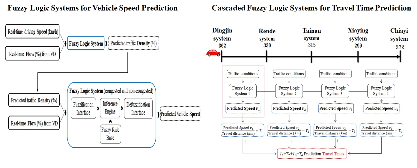
The relationship among vehicle speed, traffic flow, and traffic density on highways can be described by Greenshields models. This study focuses on the design and implementation of a fuzzy logic system for vehicle speed prediction based on Greenshields models. In the proposed approach, traffic flow and traffic density serve as input parameters, with their corresponding membership functions defined according to realistic traffic conditions. A fuzzification process transforms these inputs into meaningful fuzzy values based on the specified membership functions. The fuzzy inference mechanism then applies logical rules derived from Greenshields models to the input information, establishing decision-making laws for predicting vehicle speed as the output parameter. In the defuzzification stage, the centroid method is employed to convert the fuzzy inference results into a precise vehicle speed prediction. For practical application, the models were developed using traffic data from the southern section of Sun Yat-Sen Highway, specifically the segment between the Dingjin System and the Rende System. The speed limit for passenger cars on this highway ranges from 60 to 110 km/h, with a buffer zone permitting speeds up to 120 km/h. Traffic flow and density data were obtained from the Freeway Bureau [42] and integrated into the model design to ensure that the simulation results are stable and representative of actual traffic conditions. Cascading fuzzy systems in sequence along each highway section enables both vehicle speed prediction and travel time estimation for specified distances. The procedure for designing the fuzzy logic system is illustrated in Figure 8. Finally, we constructed an additional model using polynomial regression based on the collected data and compared its performance with that of the fuzzy logic model to verify the feasibility of the proposed approach.
3.1. Input and Output Membership Functions Setup for Greenshields Model-Based Fuzzy Logic Systems
The proposed fuzzy logic system is designed to account for two traffic conditions: congested and non-congested. In each condition, traffic flow and traffic density serve as input parameters, while vehicle speed is the output parameter. Traffic flow is defined as the number of vehicles passing through a road section per hour (veh/h), with its range expressed as a percentage of the specified full flow. Vehicle density refers to the number of vehicles per kilometer on a road section (veh/km), also expressed as a percentage of the specified full density. Vehicle speed represents the rate at which vehicles travel on the road (km/h), with a parameter range from 0 km/h to 130 km/h. Trigonometric or trapezoidal membership functions are chosen for the fuzzy sets, with ambiguous regions specified based on the domain range of collected data and constraints of each highway section. The fuzzy system, with two input parameters and one output parameter, operates in two modes: congested mode and non-congested mode. In congested mode, and to align with the Greenshields models, the input membership function for traffic flow is subdivided into thirteen levels to ensure adequate accuracy of the fuzzy logic model. These levels are: Extremely Low (EL), Very Low (VL), Low (L), Sparse (Sp), Quite Low (QL), Moderate Low (ML), Moderate (M), Moderate High (MH), Quite High (QH), Dense (De), High (H), Very High (VH), and Extremely High (EH), as presented in Table 1. The membership function and its range for traffic flow in congested mode are illustrated in Figure 9.
For traffic density in congested mode, the fuzzy domain is divided into the following levels: Moderate (M), Moderate High (MH), Quite High (QH), Dense (De), High (H), Very High (VH), and Extremely High (EH), as detailed in Table 2. The corresponding membership function and range are shown in Figure 10.
The fuzzy domain of the output membership function for vehicle speed includes the following levels: Extremely Slow (ES), Very Slow (VS), Slow (S), Steady (St), Quite Slow (QS), Moderate Slow (MS), Moderate (M), Moderate Fast (MF), Quite Fast (QF), Speedy (Sp), Fast (F), Very Fast (VF), and Extremely Fast (EF), as presented in Table 3. The membership function and its range for vehicle speed are depicted in Figure 11.
For the non-congested mode, the fuzzy domain of the membership functions for traffic flow is divided into the following levels: Extremely Low (EL), Very Low (VL), Low (L), Sparse (Sp), Quite Low (QL), Moderate Low (ML), Moderate (M), Moderate High (MH), Quite High (QH), Dense (De), High (H), Very High (VH), and Extremely High (EH), as presented in Table 4. The membership function and range values for traffic flow in non-congested mode are illustrated in Figure 12.
Similarly, the fuzzy domain of the membership function for traffic density in non-congested mode is segmented into seven levels: Extremely Low (EL), Very Low (VL), Low (L), Sparse (Sp), Quite Low (QL), Moderate Low (ML), and Moderate (M), as detailed in Table 5. The membership function and range values for traffic density are shown in Figure 13. The fuzzy domain of the output membership function for vehicle speed in non-congested mode is defined by the following levels: Extremely Slow (ES), Very Slow (VS), Slow (S), Steady (St), Quite Slow (QS), Moderate Slow (MS), Moderate (M), Moderate Fast (MF), Quite Fast (QF), Speedy (Sp), Fast (F), Very Fast (VF), and Extremely Fast (EF), as presented in Table 6. The membership function and its corresponding range for vehicle speed are depicted in Figure 14.
3.2. Inference Rule and Defuzzification
To establish the fuzzy inference relationship between inputs and outputs, a fuzzy rule base grounded in Greenshields theory is developed to capture the relationships among traffic flow, density, and vehicle speed, thereby reflecting real traffic conditions. In this study, T-norms are primarily used to perform fuzzy set logic operations, supporting the construction of fuzzy rules and inference processes to assess the similarity between fuzzy sets. Within the fuzzy rules, the intersection of fuzzy sets is represented by the minimum value, while the union operation expresses the degree of inclusiveness between two fuzzy sets using the maximum value. Two separate fuzzy rule sets are formulated for congested and non-congested conditions, as detailed in Table 7 and Table 8. The tabular representation of these rule sets helps ensure consistency, prevents contradictions, and avoids illogical rules that would not align with real-world highway traffic conditions, thereby supporting accurate vehicle speed prediction.
In the final stage of the Greenshields-based fuzzy logic system, defuzzification converts the fuzzy outputs into specific numerical values for further analysis and application. The centroid method is employed in the defuzzification process to calculate the center of the fuzzy result region, yielding a definitive and interpretable vehicle speed value.
3.3. Cascaded Fuzzy Logic Systems for Travel Time Prediction
Since Greenshields models are derived from short-range data collection and analysis, the proposed fuzzy logic system for vehicle speed prediction is effective for specific highway segments. As drivers typically travel along routes composed of several consecutive segments, each segment is equipped with its own dedicated fuzzy logic system for speed prediction. To enable travel time prediction for an entire route leading to a destination, multiple fuzzy subsystems—each based on the Greenshields model—are linked together in series to form a cascaded system. As illustrated in the flowchart of Figure 15, each pair of consecutive fuzzy logic subsystems corresponds to two sequential highway segments. Each subsystem receives current traffic flow and density data from its respective prediction scheme as inputs. Through fuzzy logic processing, the subsystem predicts the vehicle speed for that segment. Using the predicted speed, the travel time for the segment can then be estimated.
By cascading multiple fuzzy logic subsystems, each with traffic flow and density as inputs and vehicle speed as outputs, complex parameter relationships across a long-range route with multiple segments can be handled and analyzed in real-time, enabling accurate travel time prediction for long-distance highway paths. An example of the cascaded fuzzy logic system, consisting of four subsystems for current highway traffic status prediction, is shown in Figure 16. Each subsystem predicts the vehicle speed for its corresponding segment, and the required travel time for each segment is then calculated. By summing the travel times for all segments, the estimated total travel time for the specified journey is obtained, with real-time updates based on the current status of the highway.
The cascaded fuzzy logic system, designed for multiple specified segments, integrates, processes, and updates varying traffic information, thereby improving the accuracy of real-time highway travel time predictions. This approach not only allows for the processing of long-range traffic data but also dynamically adjusts the predicted travel time in response to changing traffic conditions, enhancing the system’s flexibility and adaptability.
4. Simulation Results and Discussions
In this section, simulations of the proposed Greenshields model-based fuzzy logic system for vehicle speed and travel time prediction are conducted using traffic data from a specified segment of the Sun Yat-Sen Highway in Taiwan. These simulations aim to demonstrate the reliability and effectiveness of the developed fuzzy logic models. For comparison, a conventional model is also established using regression analysis. The proposed cascaded system for long-range travel time prediction is likewise verified through simulation. The discussion of simulation results provides valuable insights that confirm the feasibility of the proposed system for vehicle speed prediction. The simulations ultimately validate the system’s accuracy, its capability to enhance prediction performance, and its flexibility in constructing a cascaded fuzzy logic system for travel time prediction across long-range routes composed of multiple highway segments.
4.1. Highway Vehicle Speed Prediction Using Greenshields Models Based Fuzzy Logic System
Traffic status data, including traffic flow and traffic density, collected from the segment between Dingjin and Rende on the Sun Yat-Sen Highway in Taiwan [42], are used to illustrate the design of Greenshields model-based fuzzy logic systems for dual-mode vehicle speed prediction. Separate fuzzy systems are developed for congested and non-congested modes to model the relationships among traffic flow, traffic density, and vehicle speed. To build an effective fuzzy system, the variable ranges are defined based on empirical data, and the model parameters are adjusted to align with actual traffic conditions on the specified highway segment.
The simulations are performed using MATLAB, which provides a visual interface for adjusting parameter values during model setup and for dynamically evaluating the performance of the fuzzy logic system throughout the design process. In the design specifications, the two input variables—traffic flow and traffic density—are expressed as percentages, ranging from 0% to 100% of their respective maximum values on the segment. The output variable, vehicle speed, ranges from 0 to 130 km/h. The relationship between vehicle speed and traffic density in the congested mode is shown in Figure 17, displaying a linear correlation consistent with the theoretical model in Figure 3. The relationship between vehicle speed and traffic flow in the congested mode is depicted in Figure 18, illustrating a quadratic relationship that corresponds to the theoretical model in Figure 4. Similarly, the curve of vehicle speed versus traffic density and the graph of vehicle speed versus traffic flow in the non-congested mode are presented in Figure 19 and Figure 20, respectively.
The results show that the fuzzy logic models are highly consistent with Greenshields’ theoretical models. Moreover, the dual-mode fuzzy logic system provides valuable insight into the dynamic traffic status at specific locations. Using this system, real-time vehicle speeds can be accurately predicted, closely approximating actual conditions. These results confirm the feasibility and effectiveness of the proposed scheme.
4.2. Greenshields Models Based on Regression Analysis
Many regression analysis methods can be applied to establish Greenshields models. In this study, polynomial regression is used to construct models based on traffic data collected from the segment between Dingjin and Rende on the Sun Yat-Sen Highway in Taiwan [42], for validation and comparison with the proposed fuzzy logic system. The regression process extracts key information from the collected data and smooths out noise present in the measurements. The resulting models in non-congested mode include the relationship curve between vehicle speed and traffic density shown in Figure 21, the graph of traffic flow versus traffic density illustrated in Figure 22, and the diagram of vehicle speed versus traffic flow presented in Figure 23.
However, regression is a slow and time-consuming process, and the models it produces are static. When conditions or the environment change, new parameters or parameter updates require a substantial amount of additional data for retraining. Despite these limitations, regression models are valuable for examining and verifying the relationships among variables. According to Greenshields’ theory, each curve provides useful insights into the relationships between vehicle speed and traffic density, traffic flow and density, and vehicle speed and traffic flow. The Greenshields models constructed through regression for the specified road segment serve as important references for validating the fuzzy logic system, evaluating its performance, and guiding model parameter adjustments.
4.3. Vehicle Speed Prediction: Tests and Discussion
A realistic simulation test in the non-congested mode was conducted using the proposed fuzzy logic system. In this test, the traffic flow input parameter was set at 40% of its maximum value, and the traffic density was set at 20%. When these parameters were fed into the fuzzy logic system, the predicted vehicle speed was approximately 102 km/h, as shown in Figure 24. For comparison, the polynomial regression model in Figure 23 predicts a vehicle speed of about 103 km/h at the same traffic flow level (40%), while the regression model in Figure 21 predicts a speed of about 100 km/h at a traffic density of 20% in the non-congested mode. The simulation results confirm the accuracy of the proposed fuzzy logic system in predicting vehicle speed. The predicted speeds are within about 1% of those generated by regression analysis methods in high-fidelity traffic scenarios. This demonstrates that the proposed system provides predictions that closely approximate actual traffic conditions, validating its feasibility for vehicle speed prediction. Another simulation was performed under a “Quite Low” traffic status scenario, where the traffic flow was set at 34% (classified as “Quite Low”) and the traffic density at 20% (classified as “Low”). Using the centroid method for defuzzification, the fuzzy logic system operating in non-congested mode predicted a vehicle speed of 101 km/h, as shown in Figure 25. This result further confirms the system’s ability to reflect realistic changes in highway traffic conditions.
For the test in congested mode, the input parameters were set with the traffic flow at 21% (classified as “Low”) and the traffic density at 89% (classified as “Very High”). As shown in Figure 26, the fuzzy logic system produced an output vehicle speed of 23.2 km/h. This outcome indicates that under congested conditions, the predicted speed aligns well with actual traffic behavior.
These results demonstrate that the fuzzy logic system accurately captures the relationships among vehicle speed, traffic flow, and traffic density. The Greenshields model-based fuzzy rules generate outputs based on the degrees of membership derived from the input values, validating the system’s effectiveness. Overall, these simulations provide further insight into traffic behavior under various conditions, reaffirming the applicability and flexibility of the designed fuzzy logic system.
4.4. Travel Time Prediction Using Greenshields Model Based Cascaded Fuzzy Logic Systems
A simulation test was conducted to evaluate travel time prediction using cascaded fuzzy logic systems for segments of the Sun Yat-Sen Highway, specifically from the Dingjin System heading north to the Chiayi System during morning rush hours on a typical working day. The route consists of four segments in sequence: Dingjin to Rende, Rende to Tainan, Tainan to Xiaying, and Xiaying to Chiayi. Each segment is equipped with a dedicated Greenshields model-based fuzzy logic system designed in advance for vehicle speed prediction. These fuzzy logic systems receive real-time traffic data—including traffic density and flow—from the Traffic Control Center for their respective segments [42]. Based on these inputs, each system predicts the vehicle speed for its segment. Using the predicted speeds and the known lengths of the segments, the estimated travel time for each segment is calculated. The total estimated travel time for the entire route from Dingjin to Chiayi is then determined by summing the segment travel times. The simulation results are presented in Table 9, showing the predicted travel times for each segment along with the corresponding traffic conditions. It is important to note that these estimates vary with changing road conditions and must be updated accordingly. The simulation confirms both the feasibility and adaptability of the cascaded fuzzy logic approach. Since each prediction relies on short-range, segment-specific traffic data, the overall travel time estimate for the planned route demonstrates a high level of accuracy.
5. Conclusions
Travel time prediction plays a crucial role in ITS, supporting efficient route planning, minimizing travel costs, optimizing traffic flow, reducing delays, and alleviating congestion. It helps travelers make informed decisions about departure times and routes, ultimately saving time and fuel while lowering environmental impact. In this paper, we propose a cascaded fuzzy logic system for predicting the required travel time of a planned highway route. The system is divided into multiple fuzzy logic subsystems, with each subsystem responsible for forecasting travel time on a specific highway segment. Each fuzzy logic subsystem operates in either congested or non-congested mode and is designed to account for road conditions that influence input traffic status. By integrating Greenshields models, the system uses fuzzy sets and rules to address the uncertainties inherent in traffic flow and density on the specified highway segments, enabling more accurate vehicle speed predictions. Each fuzzy logic subsystem comprises multiple Greenshields model-based fuzzy modules, configured to handle either congested or non-congested conditions. By combining knowledge from Greenshields models with real-world traffic data, these subsystems provide reliable and efficient vehicle speed predictions. Simulations were conducted for the designed fuzzy logic subsystems and compared with polynomial regression models using collected traffic data from the specified segments of the Sun Yat-Sen Highway. The results demonstrate that the fuzzy logic subsystems deliver effective and accurate travel time predictions, adapting to variations in speed, flow, and density across different road sections. Finally, the cascaded fuzzy logic system is applied for route planning along the specified highway segments. Predicted travel times for each segment are combined to estimate the total travel time for the route. The results confirm that the cascaded fuzzy logic system accurately reflects actual traffic conditions and is capable of forecasting long-range travel times.
Author Contributions
Conceptualization, M.J.H. and Y.X.Z.; methodology, M.J.H.; software, Y.X.Z.; validation, M.J.H. and Y.X.Z.; formal analysis, M.J.H.; resources, Y.X.Z.; writing—original draft preparation, M.J.H. and Y.X.Z.; writing—review and editing, M.J.H.; supervision, M.J.H. All authors have read and agreed to the published version of the manuscript.
Funding
This research received no external funding.
Conflicts of Interest
The authors declare no conflicts of interest.
References
- Freeway Bureau MOTC, Monthly Statistics of Million Vehicle Kilometers, [Online]. Available online: https://www.freeway.gov.tw/Publish.aspx?cnid=1656 (accessed on 8 May 2025).
- Thakur, A.; Malekian, R. Fog computing for detecting vehicular congestion, an internet of vehicles based approach: A review. IEEE Intelligent Transportation Systems Magazine 2019, 11, 8–16. [Google Scholar] [CrossRef]
- Alsrehin, N.O.; Klaib, A.F.; Magableh, A. Intelligent transportation and control systems using data mining and machine learning techniques: a comprehensive study. IEEE Access 1019, 7, 49830–49857. [Google Scholar] [CrossRef]
- Ting, P.Y.; et al. Freeway travel time prediction using deep hybrid model – taking Sun Yat-Sen Freeway as an example. IEEE Transactions on Vehicular Technology 2020, 69, 8257–8266. [Google Scholar] [CrossRef]
- Li, L.; Lin, H.; Wan, J.; Ma, Z.; Wang, H. MF-TCPV: A machine learning and fuzzy comprehensive evaluation-based framework for traffic congestion prediction and visualization. IEEE Access 2020, 8, 227113–227125. [Google Scholar] [CrossRef]
- Iyer, L.S. AI enabled applications towards intelligent transportation. Transportation Engineering 2021, 5. [Google Scholar] [CrossRef]
- Rashid, A.B.; Kausik, A.K. AI revolutionizing industries worldwide: A comprehensive overview of its diverse applications. Hybrid Advances 2024, 7. [Google Scholar] [CrossRef]
- U.S. Government Accountability Office. In Intelligent Transportation Systems: Benefits Related to Traffic Congestion and Safety Can Be Limited by Various Factors; GAO-23-105740. 2023. Available online: https://www.gao.gov/products/gao-23-105740.
- Nesa, M.; Yoon, Y. Speed prediction and nearby road impact analysis using machine learning and ensemble of explainable AI techniques. Sci Rep. 2024, 14, 25208. [Google Scholar] [CrossRef]
- Qiu, B.; Fan, W. Machine learning based short-term travel time prediction: numerical results and comparative analyses. Sustainability 2021, 13, 7454. [Google Scholar] [CrossRef]
- Zhang, X.; Rice, J.A. Short-term travel time prediction. Transp. Res. C, Emerg. Technol. 2003, 11, 187210. [Google Scholar] [CrossRef]
- Liu, X.; Xu, J.; Li, M.; Wei, L.; Ru, H. General-logistic-based speed-density relationship model incorporating the effect of heavy vehicles. Math. Problems Eng. 2019, 6039846. [Google Scholar] [CrossRef]
- Kachroo, P.; Sastry, S. Traffic assignment using a density-based travel-time function for intelligent transportation systems. IEEE Transactions on Intelligent Transportation Systems 2016, 17, 1438–1447. [Google Scholar] [CrossRef]
- Soriguera, F.; Martínez-Díaz, M. Freeway travel time information from input- output vehicle counts: a drift correction method based on AVI data. IEEE Transactions on Intelligent Transportation Systems 2021, 22, 5749–5761. [Google Scholar] [CrossRef]
- Liu, X.; Jinliang, X.; Li, M.; Wei, L.; Han, R. General-logistic-based speed-density relationship model incorporating the effect of heavy vehicles. Mathematical Problems in Engineering 2019, 1–10. [Google Scholar] [CrossRef]
- Zhang, S.; Ma, J.; Geng, B.; Wang, H.B. Traffic flow prediction with a multi-dimensional feature input: A new method based on attention mechanisms. Electronic Research Archive 2024, 32, 979–1002. [Google Scholar] [CrossRef]
- Kühne, R. Foundation of traffic flow theory I: Greenshields legacy highway traffic. in Proceedings Symposium on the Fundamental Diagram: 75 years. TRB Traffic Flow Theory and Characteristics Committee Summer Meeting and Symposium on the Fundamental Diagram: 75 years (“Greenshields75 Symposium”), Woods Hole, Massachusetts, USA, 08 07 2008 – 10 07 2008.
- Xu, Y.; Kong, Q.J.; Klette, R.; Liu, Y. Accurate and interpretable Bayesian MARS for traffic flow prediction. IEEE Transactions on Intelligent Transportation Systems 2014, 15, 2457–2469. [Google Scholar] [CrossRef]
- Dell’Acqua, P.; Bellotti, F.; Berta, R.; De Gloria, A. Time-aware multivariate nearest neighbor regression methods for traffic flow prediction. IEEE Transactions on Intelligent Transportation Systems 2015, 16, 3393–3402. [Google Scholar] [CrossRef]
- Liu, R.; Shin, S.Y. A review of traffic flow prediction methods in intelligent transportation system construction. Appl. Sci. 2025, 15, 3866. [Google Scholar] [CrossRef]
- Van Der Voort, M.; Dougherty, M.; Watson, S. Combining Kohonen maps with ARIMA time series models to forecast traffic flow. Transp. Res. C, Emerg. Technol. 1996, 4, 307318. [Google Scholar] [CrossRef]
- Zhao, Z.; Chen, W.; Yue, H.; Liu, Z. “A novel short-term traffic forecast model based on travel distance estimation and ARIMA,” In 2016 Chinese Control and Decision Conference (CCDC 2016), Yinchuan, China 2016, 6270-6275. [CrossRef]
- Oh, S.D.; Kim, Y.J.; Hong, J.S. Urban traffic flow prediction system using a multifactor pattern recognition model. IEEE Transactions on Intelligent Transportation Systems 2015, 16, 2744–2755. [Google Scholar] [CrossRef]
- Messmer, A.; Papageorgiou, M. A mixed extended Kalman filter–maximum likelihood approach for real-time freeway traffic state estimation. Transp. Res. Part C Emerg. Technol. 2004, 12, 209–238. [Google Scholar]
- Zhao, M.; Roncoli, C.; Wang, Y.; Bekiaris-Liberis, N.; Guo, J.; Cheng, S. Generic approaches to estimating freeway traffic state and percentage of connected vehicles with fixed and mobile sensing. IEEE Transactions on Intelligent Transportation Systems 2022, 23, 13155–13177. [Google Scholar] [CrossRef]
- Zhu, Y.; Wu, Q.; Xiao, N. Research on highway traffic flow prediction model and decision-making method. Sci Rep. 2022, 12, 19919. [Google Scholar] [CrossRef] [PubMed]
- Wu, C.H.; Ho, J.M.; Lee, D.T. Travel-time prediction with support vector regression. IEEE Transactions on Intelligent Transportation Systems 2004, 5, 276–281. [Google Scholar] [CrossRef]
- Zhang, X.; Rice, J.A. Short-term travel time prediction. Transp. Res. C, Emerg. Technol. 2003, 11, 187210. [Google Scholar] [CrossRef]
- Khosravi, A.; Mazloumi, E.; Nahavandi, S.; Creighton, D.; Van Lint, J.W.C. A genetic algorithm-based method for improving quality of travel time prediction intervals. Transp. Res. C, Emerg. Technol. 2011, 19, 13641376. [Google Scholar] [CrossRef]
- Yang, M.; Chen, C.; Wang, L.; Yan, X.; Zhou, L. Bus arrival time prediction using support vector machine with genetic algorithm. Neural Network World 2016, 26, 205–217. [Google Scholar] [CrossRef]
- Lagos, F.; Moreno, S.; Yushimito, W.F.; Brstilo, T. Urban origin–destination travel time estimation using K-nearest-neighbor-based methods. Mathematics 2024, 12, 1255. [Google Scholar] [CrossRef]
- Yu, B.; Lam, W.H.; Tam, M.L. Bus arrival time prediction at bus stop with multiple routes. Transp. Res. Part C: Emerg. Technologies 2011, 19, 1157–1170. [Google Scholar] [CrossRef]
- Innamaa, S. Short-term prediction of travel time using neural networks on an interurban highway. Transportation 2005, 32, 649669. [Google Scholar] [CrossRef]
- Derrow-Pinion, A.; et al. ETA prediction with graph neural networks in Google maps. In Proc. 30th ACM Int. Conf. Inf. Knowl. Manage., Oct. 2021, 3767-3776.
- Zhao, J.; et al. et al. Truck traffic speed prediction under non-recurrent congestion: Based on optimized deep learning algorithms and GPS data. IEEE Access 2019, 7, 9116–9127. [Google Scholar] [CrossRef]
- Tang, J.; Liu, F.; Zou, Y.; Zhang, W.; Wang, Y. An improved fuzzy neural network for traffic speed prediction considering periodic characteristic. IEEE Trans. Intell. Transp. Syst. 2017, 18, 23402350. [Google Scholar] [CrossRef]
- Tomar, A.S.; Singh, M.; Sharma, G.; Arya, K.V. Traffic management using logistic regression with fuzzy logic. Procedia Computer Science 2018, 132, 451–460. [Google Scholar] [CrossRef]
- Abberley, L.; Crockett, K.; Cheng, J. Modeling road congestion using a fuzzy system and real-world data for connected and autonomous vehicles. In 2019 Wireless Days (WD); Manchester, UK, 2019; pp. 1–8. [CrossRef]
- Hao, M.J.; Hsieh, B.Y. Greenshields model-based fuzzy system for predicting traffic congestion on highways. IEEE Access 2024, 12, 115868–115882. [Google Scholar] [CrossRef]
- Tseng, F.H.; Hsueh, J.H.; Tseng, C.W.; Yang, Y.T.; Chao, H.C.; Chou, L.D. Congestion prediction with big data for real-time highway traffic. IEEE Access 2018, 6, 57311–57323. [Google Scholar] [CrossRef]
- Kumar, N.; Rahman, S.S.; Dhakad, N. Fuzzy inference enabled deep reinforcement learning-based traffic light control for intelligent transportation system. IEEE Transactions on Intelligent Transportation Systems 2021, 22, 4919–4928. [Google Scholar] [CrossRef]
- Huang, C.N. Greenshields Model-based Travel Time Estimation for Traffic on Highway. M. S. Thesis, Dept. Computer and Commun. Eng. National Kaohsiung Univ. of Sci. and Technol., Kaohsiung, Taiwan, 2019.
- Weisberg, S. Applied Linear Regression, 4th ed., John Wiley & Sons Inc.: Hoboken, New Jersey, USA, 2014.
- Bates, D.M.; Watts, D.G. Nonlinear Regression Analysis and Its Applications, John Wiley & Sons Inc.: New York, USA, 1988.
- Zadeh, L.A. Fuzzy sets. Information and Control 1965, 8, 338–353. [Google Scholar] [CrossRef]
- Chen, G.; Pham, T.T. Fuzzy-sets, Fuzzy-logic, and-Fuzzy-control-systems; CRC Press: N.W. Corporate Blvd., Boca Raton, Florida, USA, 2001. [Google Scholar]
Figure 1.
Illustration of various highway detectors.
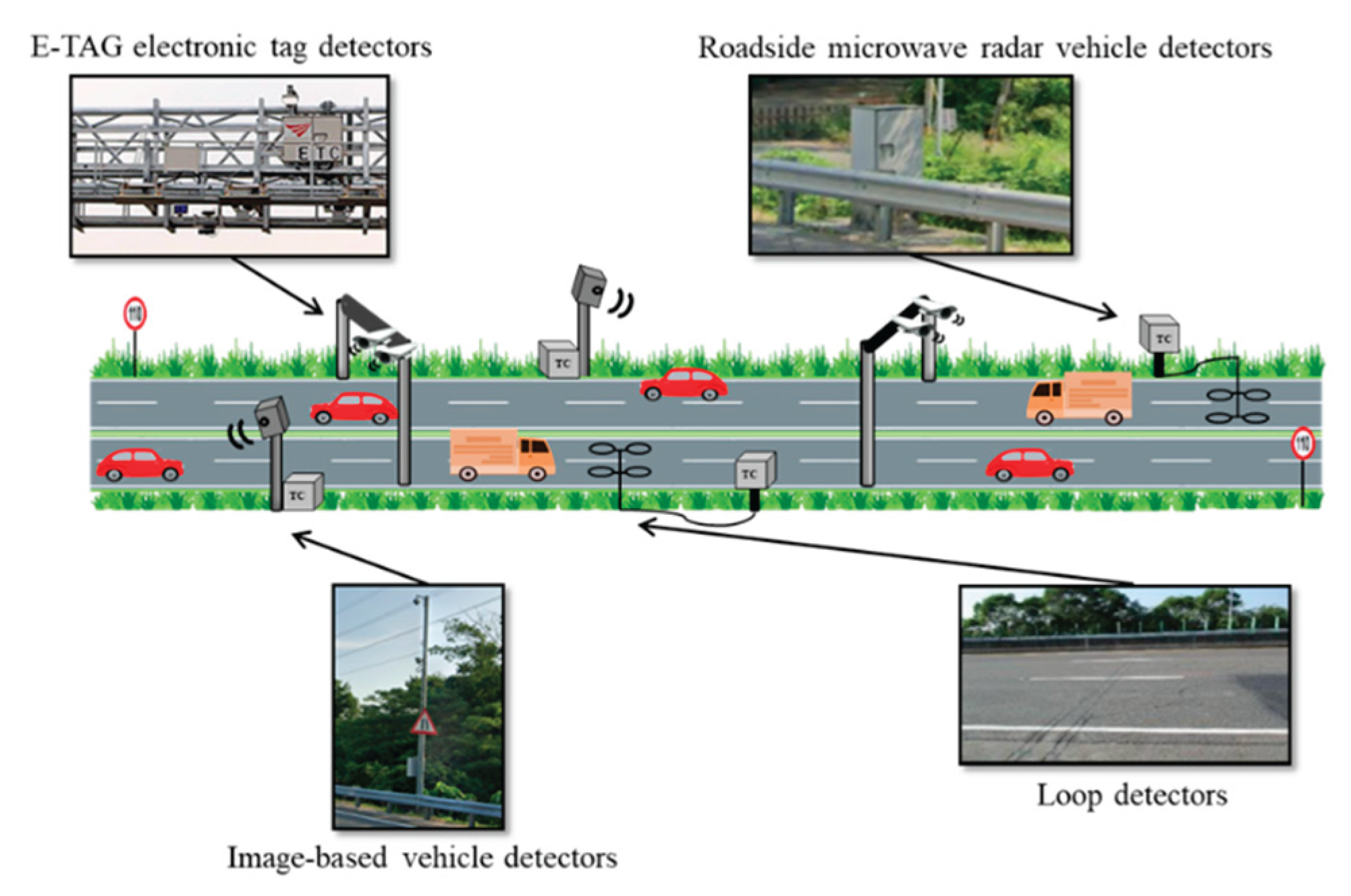
Figure 2.
Traffic flow vs. traffic density curve of the Greenshields model.
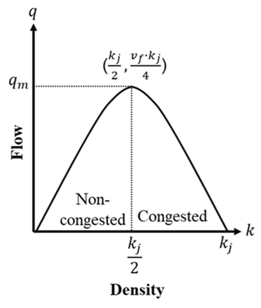
Figure 3.
Vehicle speed vs. traffic density curve of the Greenshields model.
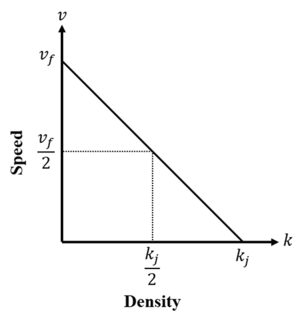
Figure 4.
Vehicle speed vs. traffic flow curve of the Greenshields model.
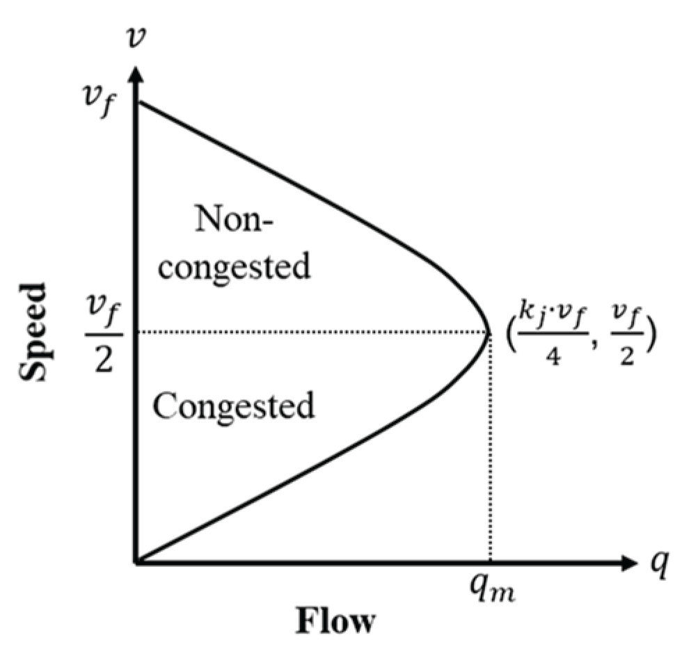
Figure 5.
Basic structure of a fuzzy logic system.
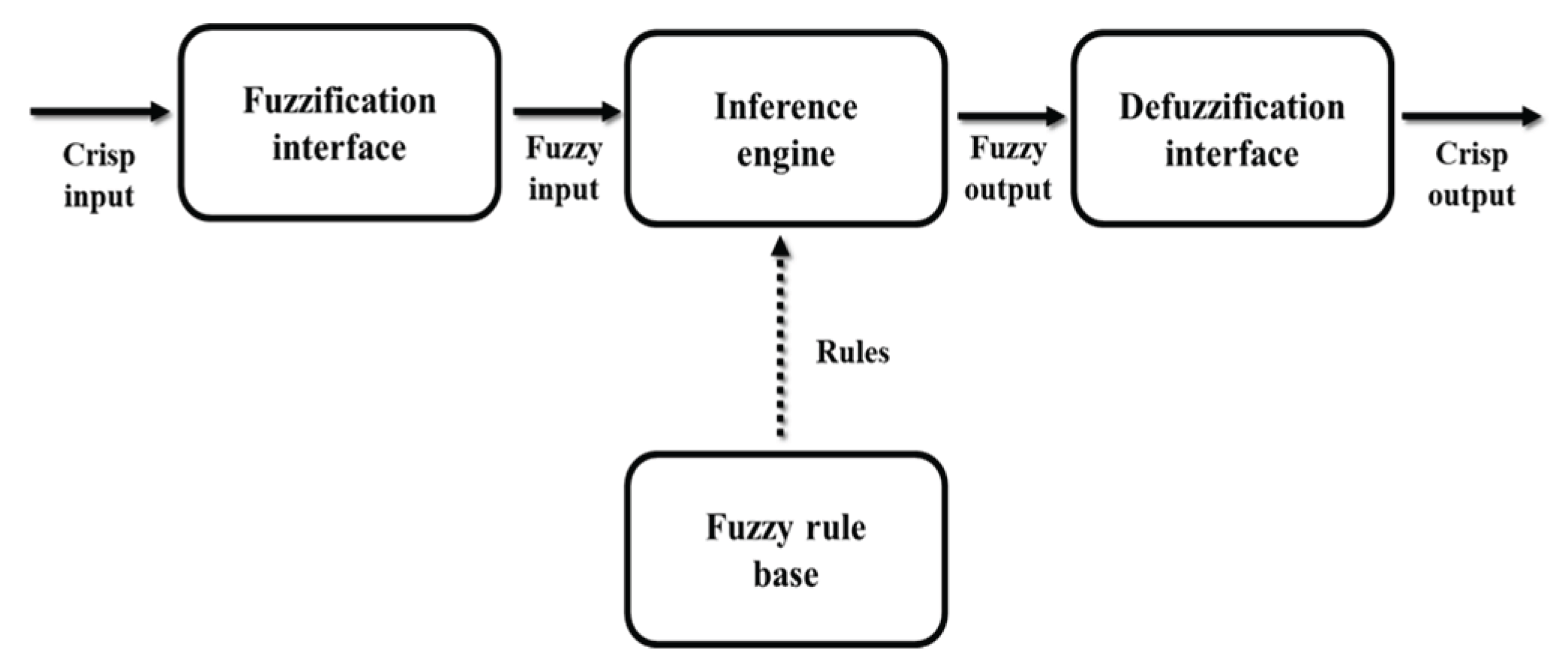
Figure 6.
Trapezoidal membership function.
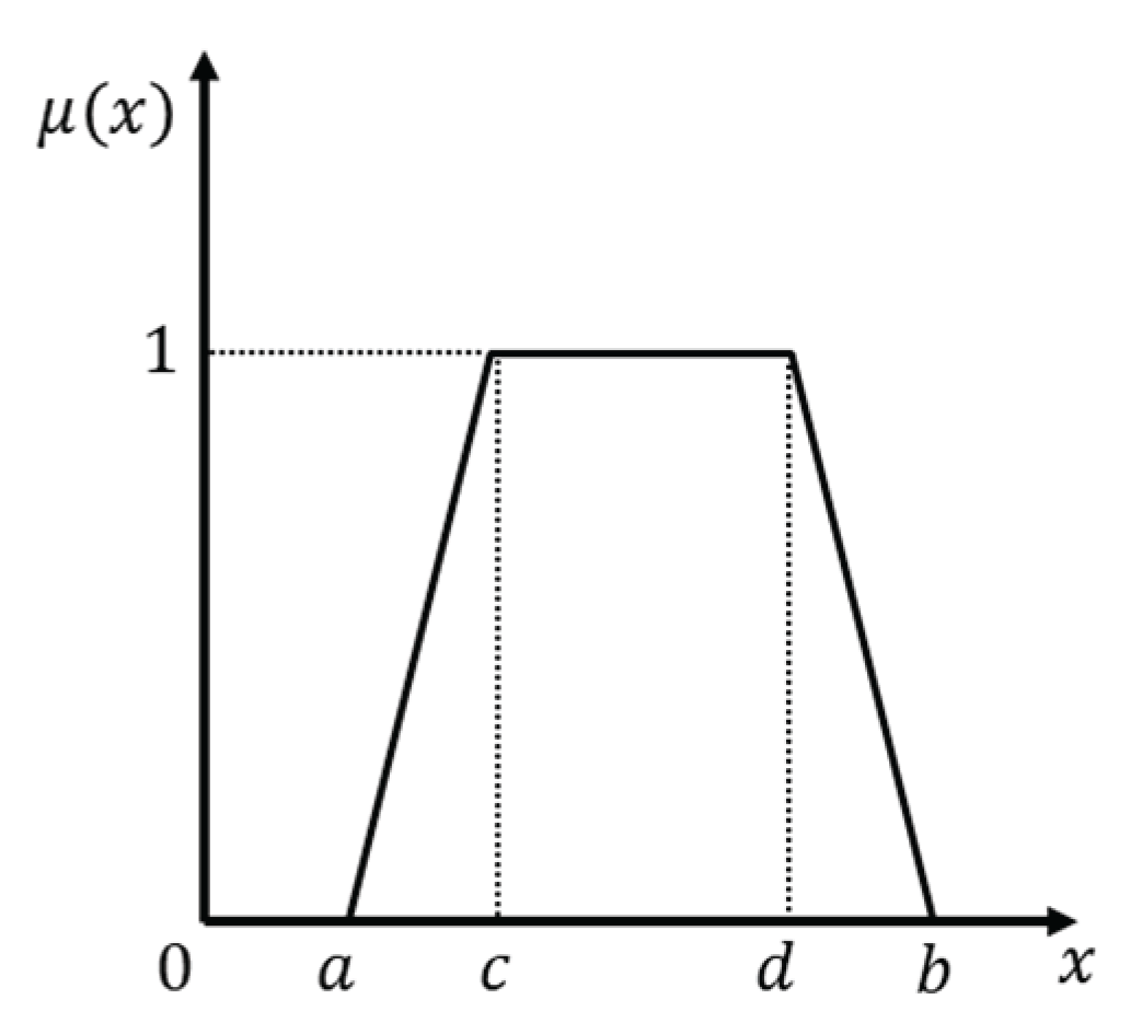
Figure 7.
Gaussian membership function.
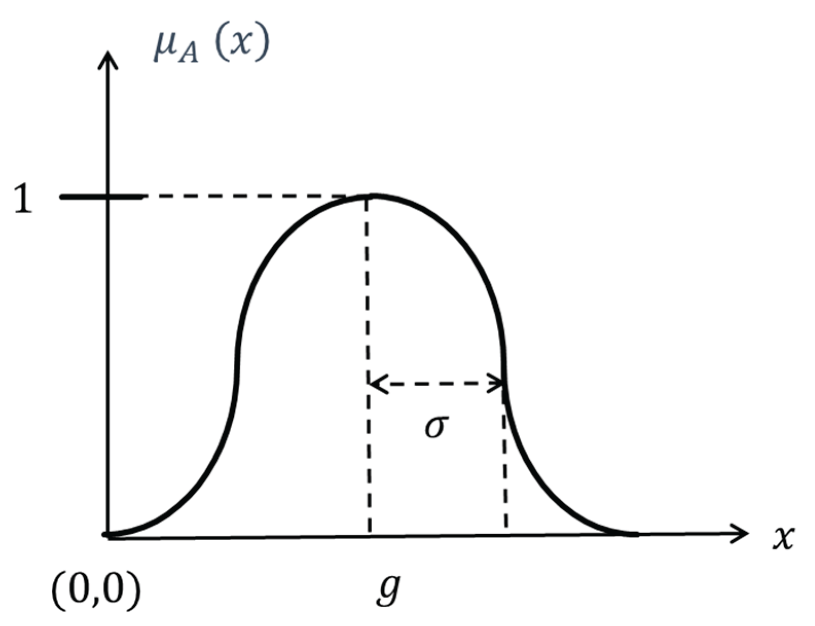
Figure 8.
Architecture of a fuzzy logic system for vehicle speed prediction.

Figure 9.
Membership function of traffic flow and its range values in congested mode.
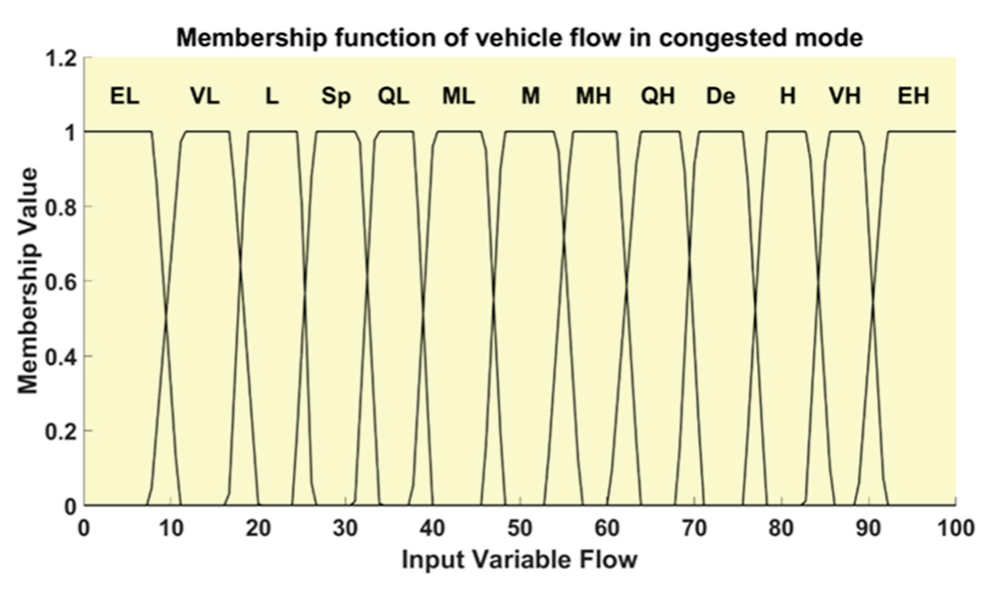
Figure 10.
Membership function of traffic density and its range values in congested mode.

Figure 11.
Membership function of traffic speed and its range values in congested mode.
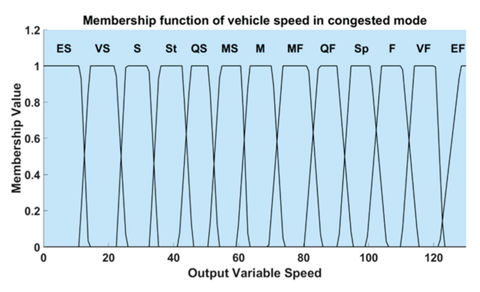
Figure 12.
Membership function of traffic flow and its range values in non-congested mode.
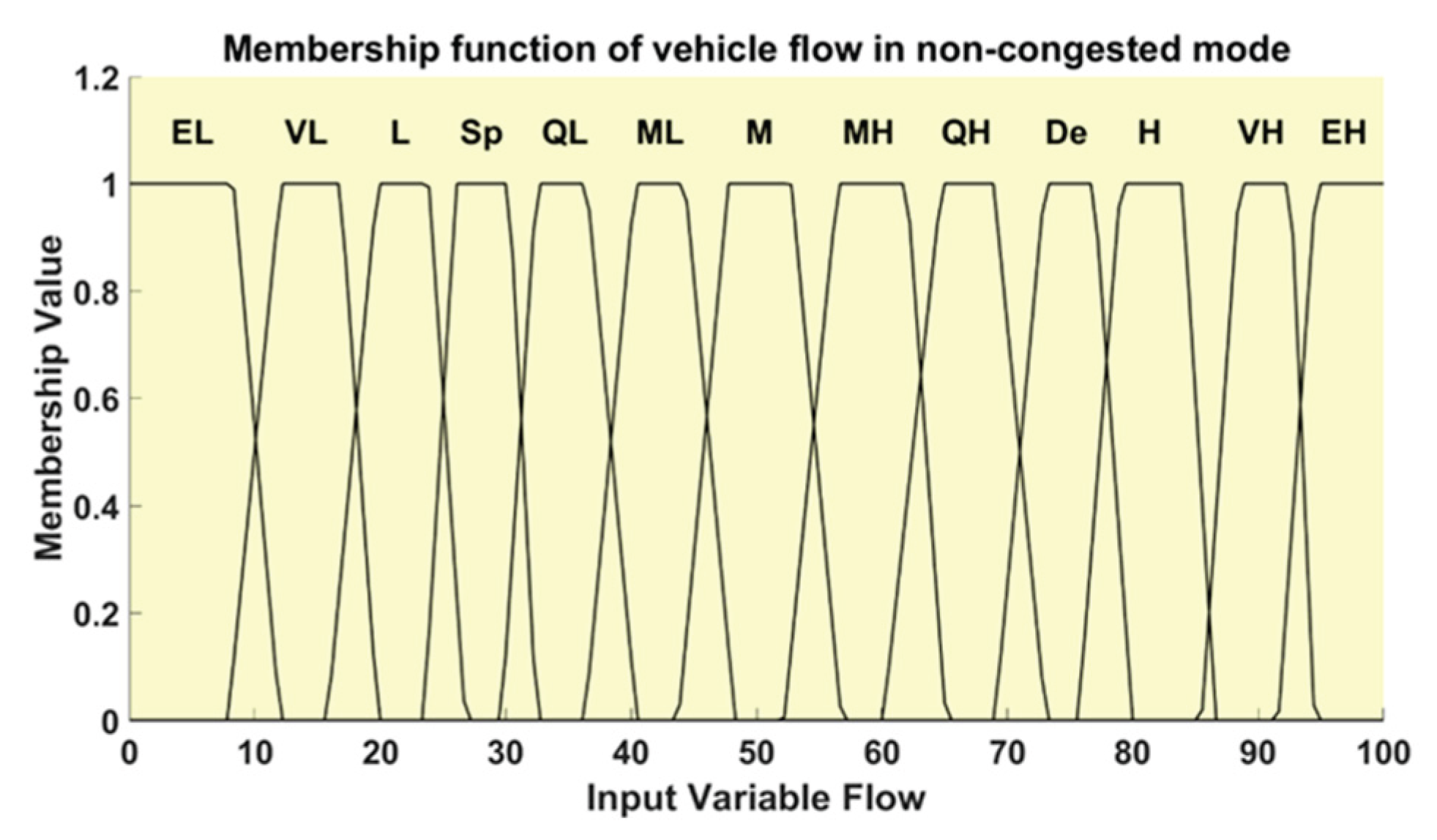
Figure 13.
Membership function of traffic density and its range values in non-congested mode.
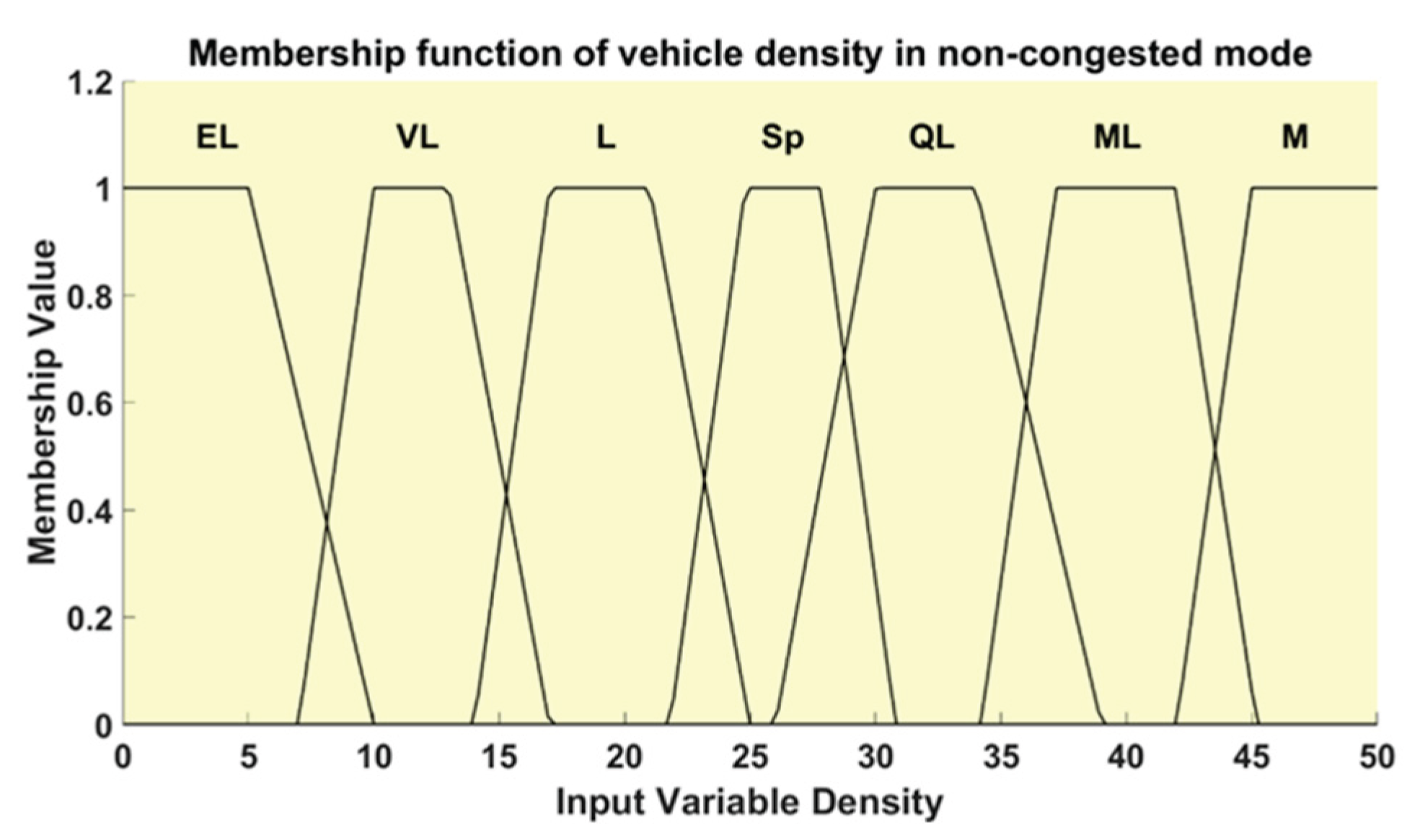
Figure 14.
Membership function of vehicle speed and its range values in non-congested mode.
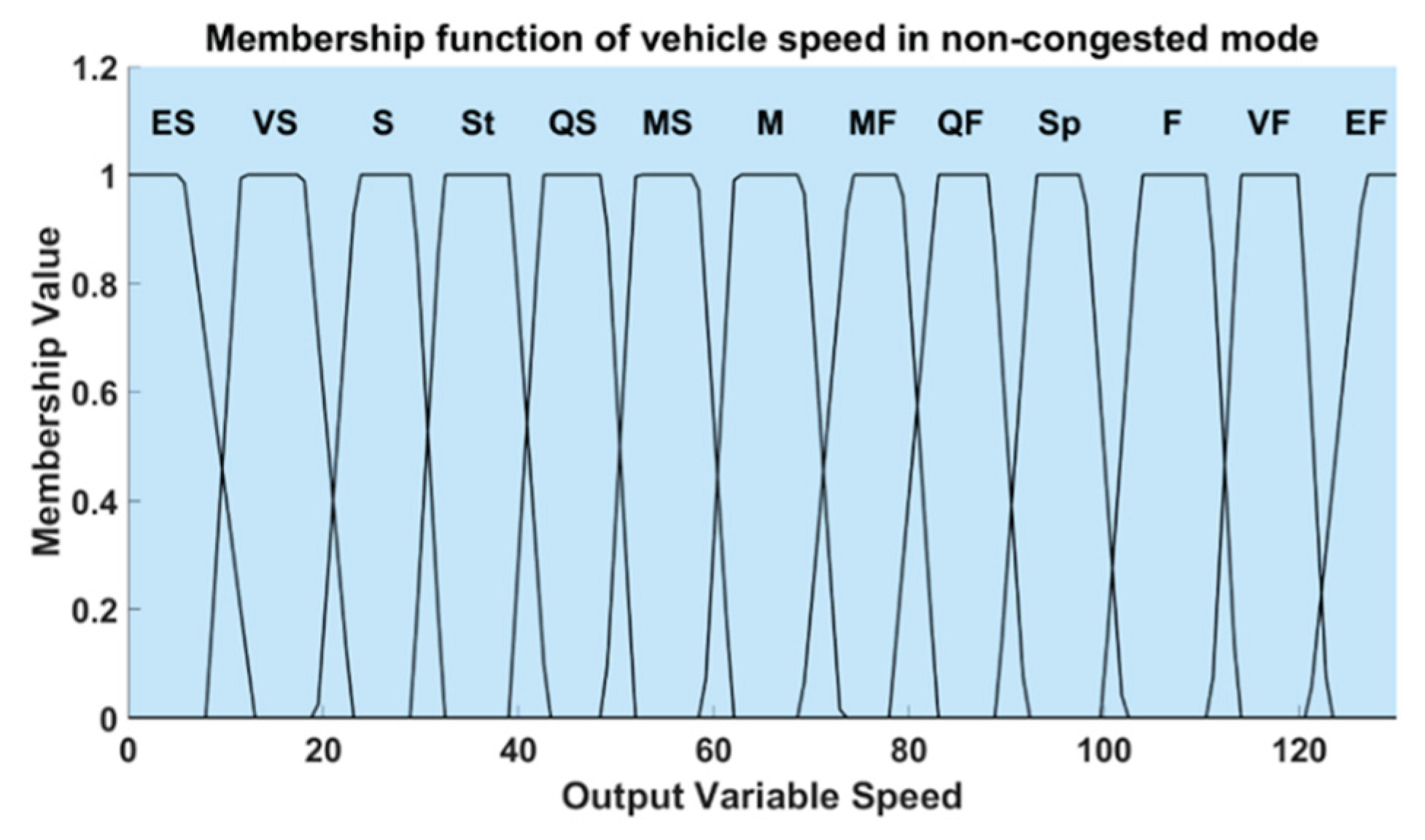
Figure 15.
Schematic diagram of a single fuzzy logic system for vehicle speed prediction.
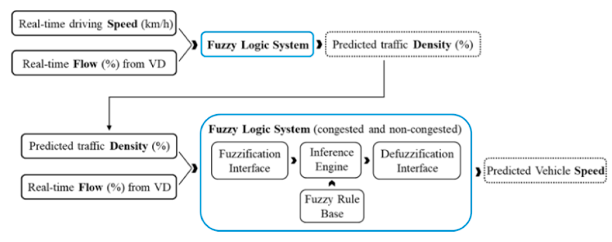
Figure 16.
Schematic diagram of a cascaded fuzzy logic system for travel-time prediction.
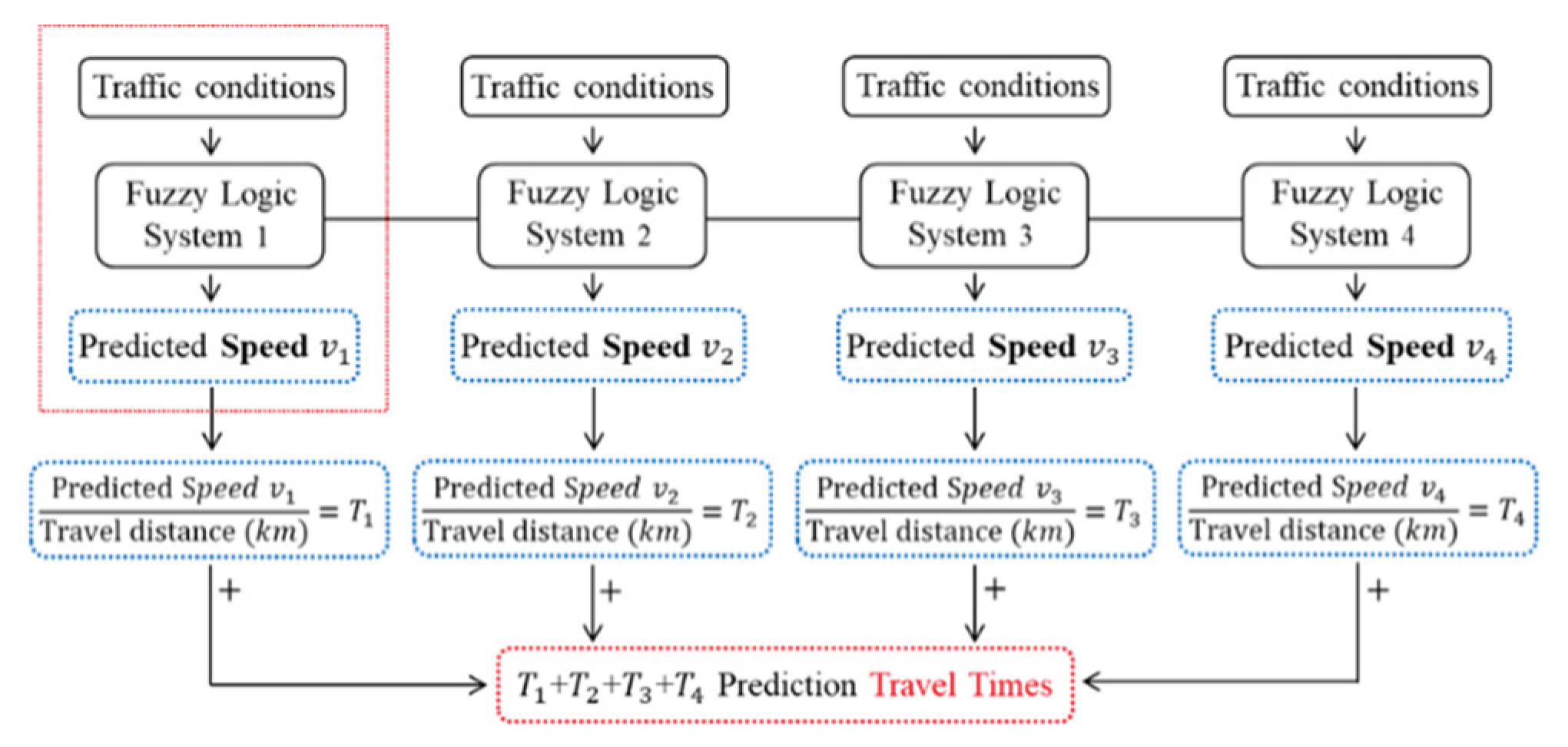
Figure 17.
Relationship curve between vehicle speed and traffic density in congested mode.
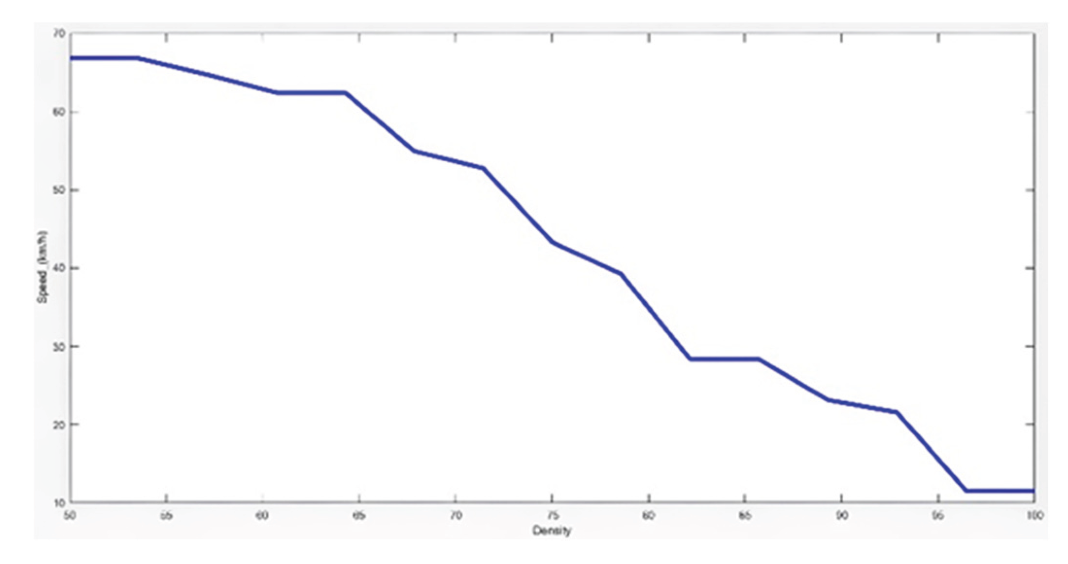
Figure 18.
Relationship curve between vehicle speed and traffic flow in congested mode.
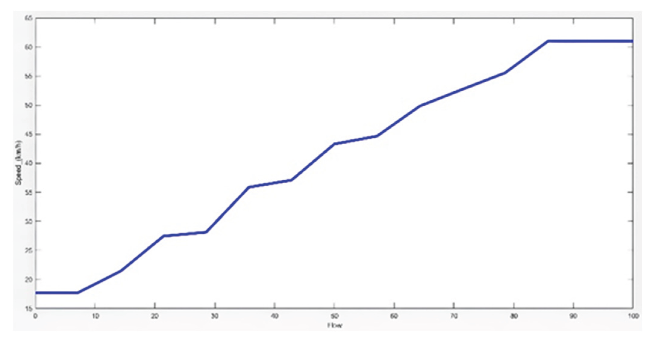
Figure 19.
Relationship curve between vehicle speed and traffic density in non-congested mode.
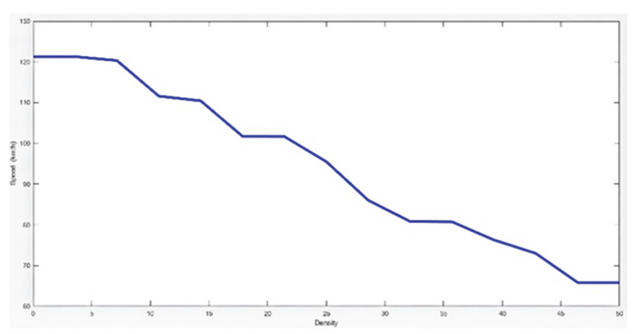
Figure 20.
Relationship curve between vehicle speed and traffic flow in non-congested mode.
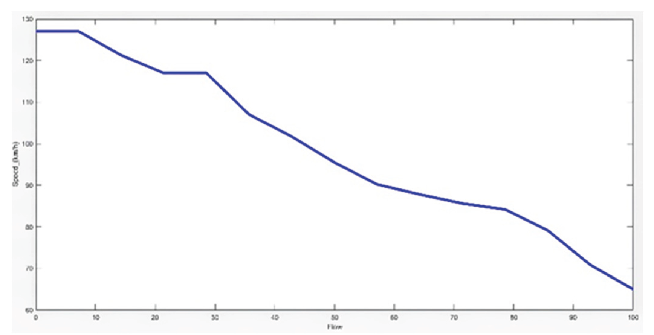
Figure 21.
Relation graphs between vehicle speed and traffic density in non-congested mode: collected data and regression curve.
Figure 21.
Relation graphs between vehicle speed and traffic density in non-congested mode: collected data and regression curve.
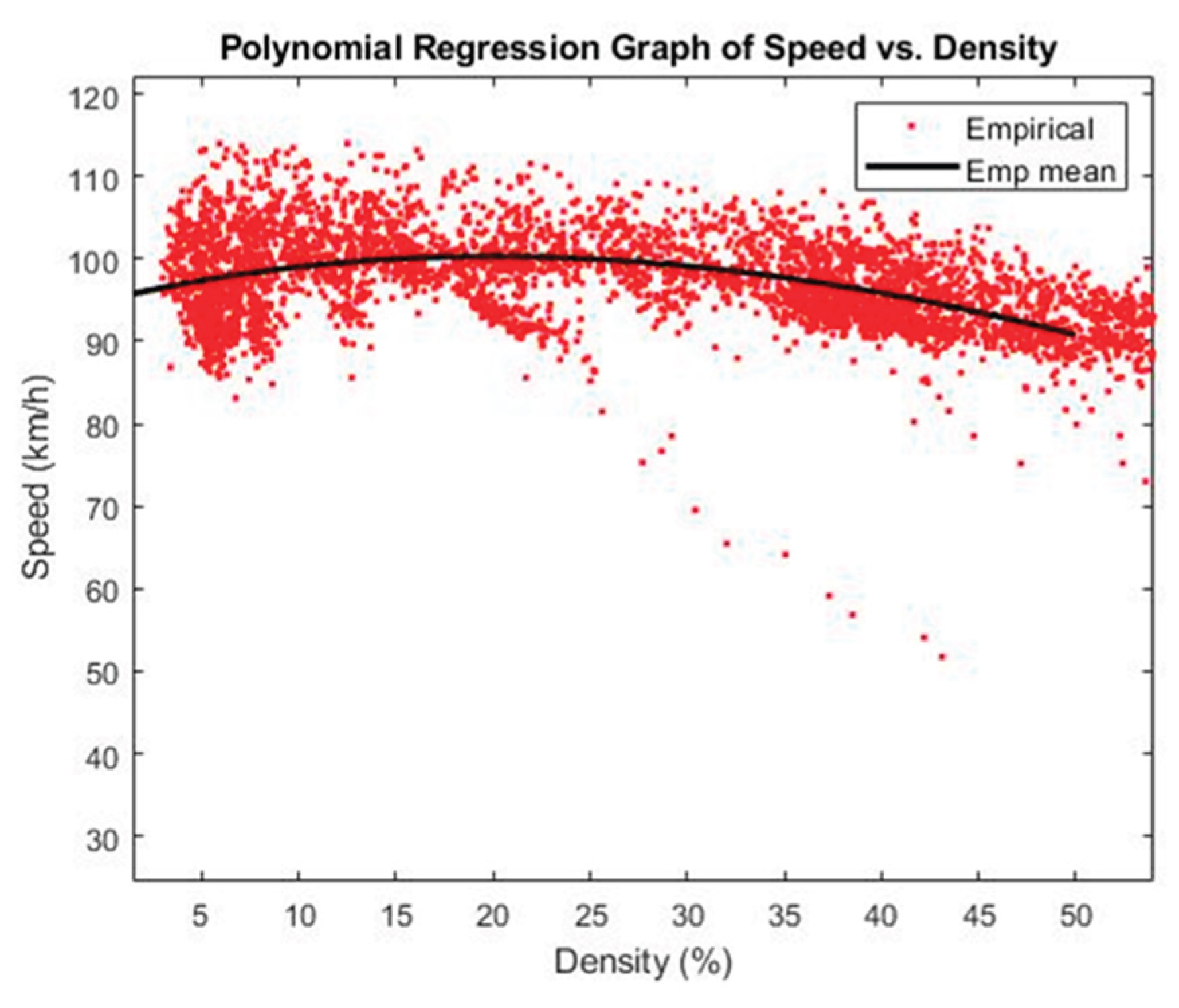
Figure 22.
Relation graphs between traffic flow and traffic density in non-congested mode: collected data and regression curve.
Figure 22.
Relation graphs between traffic flow and traffic density in non-congested mode: collected data and regression curve.
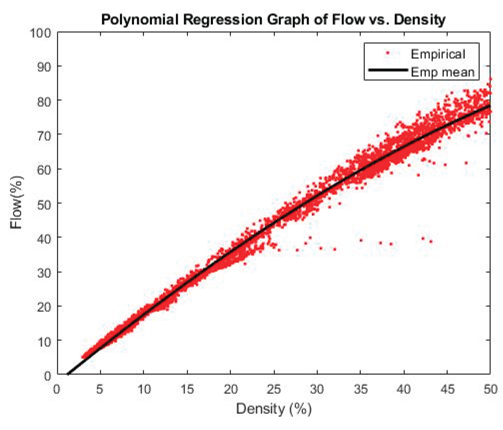
Figure 23.
Relation graphs between vehicle speed and traffic flow in non-congested mode: collected data and regression curve.
Figure 23.
Relation graphs between vehicle speed and traffic flow in non-congested mode: collected data and regression curve.
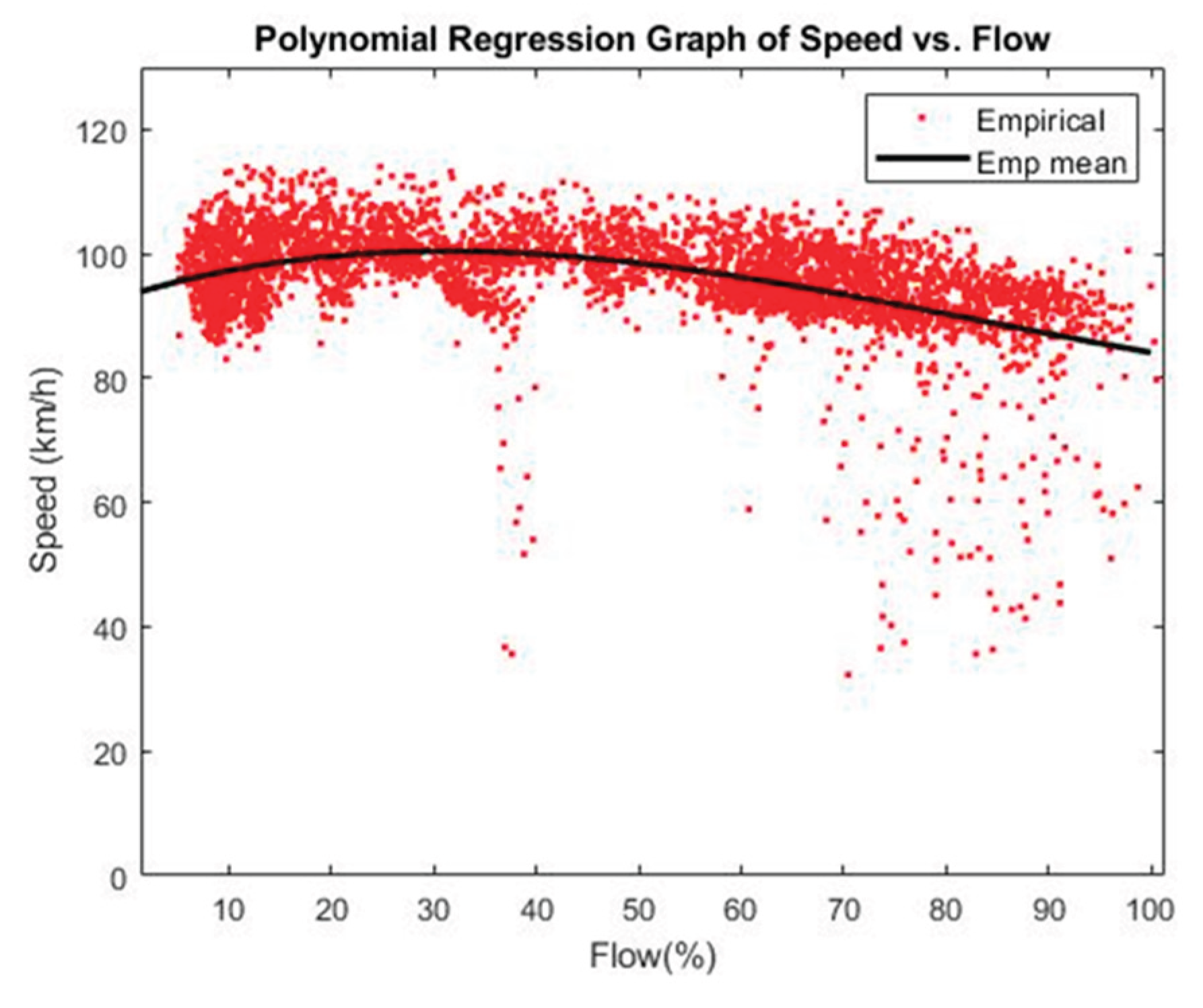
Figure 24.
Defuzzification of the proposed fuzzy logic system in non-congested mode with traffic flow at 40% and traffic density at 20%.
Figure 24.
Defuzzification of the proposed fuzzy logic system in non-congested mode with traffic flow at 40% and traffic density at 20%.
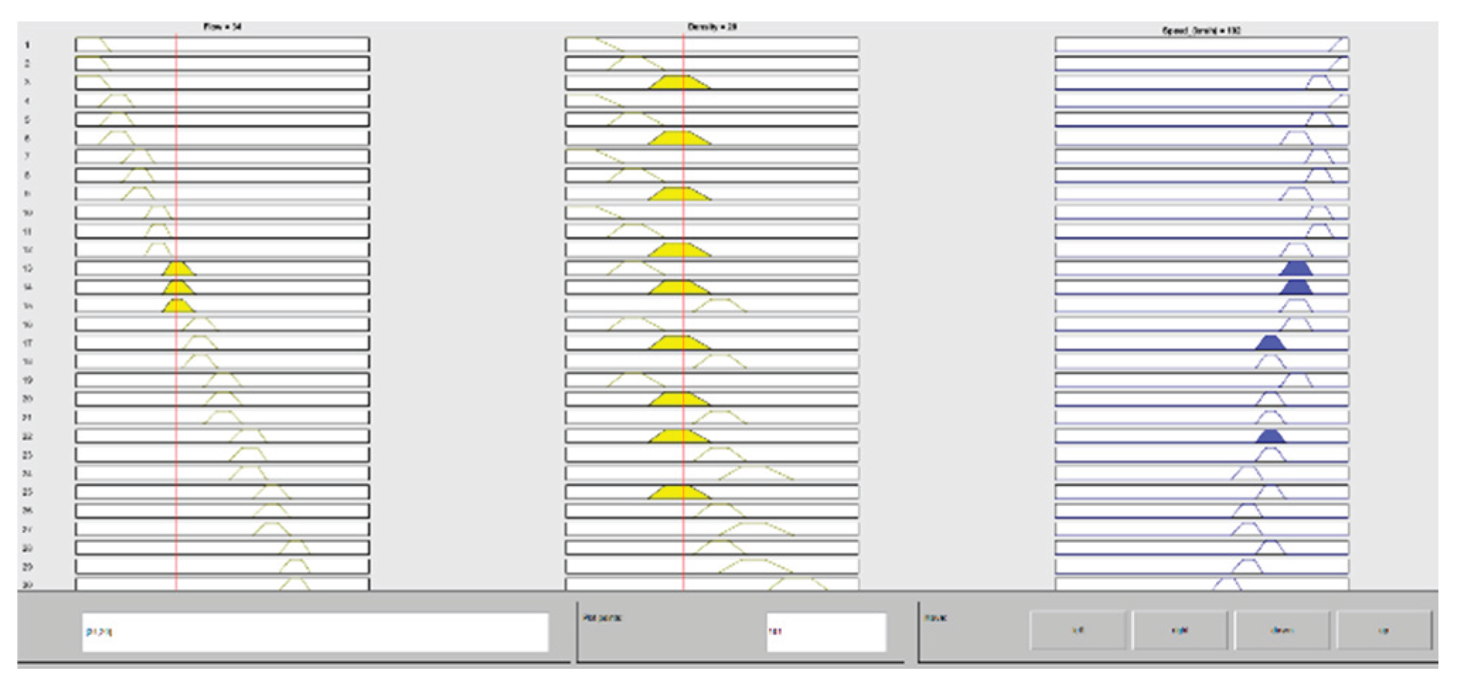
Figure 25.
Defuzzification of the proposed fuzzy logic system in non-congested mode with traffic flow at 34% and traffic density at 20%.
Figure 25.
Defuzzification of the proposed fuzzy logic system in non-congested mode with traffic flow at 34% and traffic density at 20%.
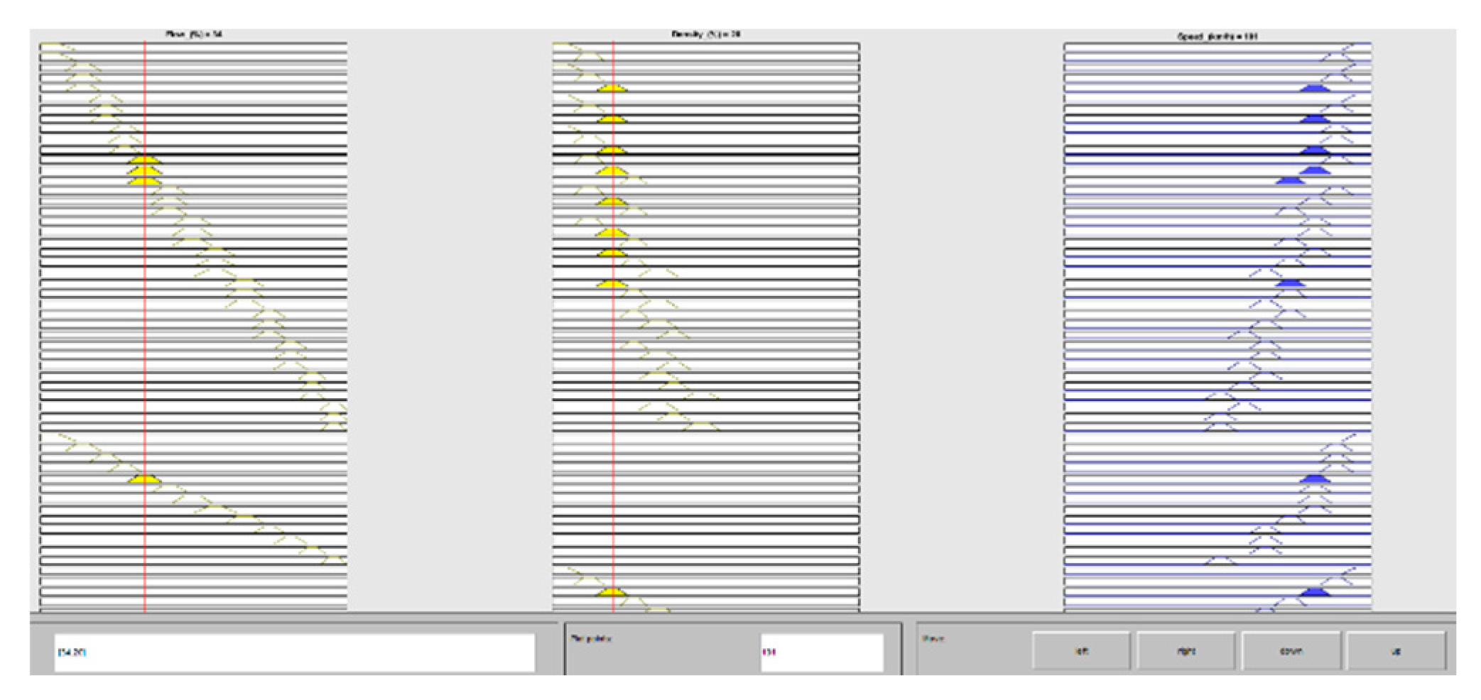
Figure 26.
Defuzzification of the proposed fuzzy logic system in congested mode with traffic flow at 21% and traffic density at 89%.
Figure 26.
Defuzzification of the proposed fuzzy logic system in congested mode with traffic flow at 21% and traffic density at 89%.
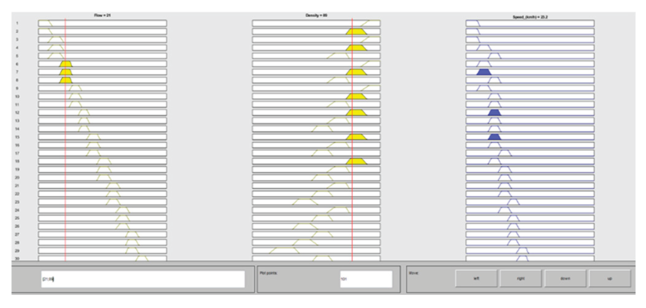

Table 1.
Membership function of traffic flow and its range values in congested mode.
| Traffic Flow (veh/h) | Percentage of Traffic Flow (%) |
|---|---|
|
Extremely Low (EL) Very Low (VL) Low flow (L) Sparse (Sp) Quite Low (QL) Moderate Low (ML) Moderate (M) Moderate High (MH) Quite High (QH) Dense (De) High (H) Very High (VH) Extremely High (EH) |
0~11 8~20 17~26 24~34 31~40 38~48 46~57 53~64 60~71 69~78 76~86 83~92 89~100 |
Table 2.
Membership function of traffic density and its range values in congested mode.
| Traffic Density (veh/km) | Percentage of Density (%) |
|---|---|
|
Moderate (M) Moderate High (MH) Quite High (QH) Dense (De) High (H) Very High (VH) Extremely High (EH) |
50~60 57~68 66~76 73~82 80~88 87~95 92~100 |
Table 3.
Membership function of vehicle speed and its range values in congested mode.
| Vehicle Speed (km/h) | Mapping Interval (km) |
|---|---|
| Extremely Slow (ES) | 0~14 |
| Very Slow (VS) | 11~26 |
| Slow (S) | 22~35 |
| Steady (St) | 33~46 |
|
Quite Slow (QS) Moderate Slow (MS) Moderate (M) Moderate Fast (MF) Quite Fast (QF) Speedy (Sp) Fast (F) Very Fast (VF) Extremely Fast (EF) |
42~54 51~63 60~74 69~85 80~95 91~106 99~115 110~123 122~130 |
Table 4.
Membership function of traffic flow and its range values in non-congested mode.
| Traffic Flow (veh/h) | Percentage of Traffic Flow (%) |
|---|---|
|
Extremely (EL) Very Low (VL) Low (L) Sparse (Sp) Quite Low (QL) Moderate Low (ML) Moderate (M) Moderate High (MH) Quite High (QH) Dense (De) High (H) Very High (VH) Extremely High (EH) |
0~12 8~20 16~27 23~32 30~40 36~48 44~57 52~65 60~73 69~80 76~87 86~95 92~100 |
Table 5.
Membership function of traffic density and its range values in non-congested mode.
| Traffic Density (veh/km) | Percentage of Density (%) |
|---|---|
| Extremely Low (EL) | 0~10 |
| Very Low (VL) | 7~17 |
| Low (L) | 14~25 |
| Sparse (Sp) | 22~31 |
|
Quite Low (QL) Moderate Low (ML) Moderate (M) |
26~39 34~45 42~50 |
Table 6.
Membership function of vehicle speed and its range values in non-congested mode.
| Vehicle Speed (km/h) | Mapping Interval (km) |
|---|---|
| Extremely Slow (ES) | 0~13 |
| Very Slow (VS) | 8~23 |
| Slow (S) | 19~32 |
| Steady (St) | 29~43 |
|
Quite Slow (QS) Moderate Slow (MS) Moderate (M) Moderate Fast (MF) Quite Fast (QF) Speedy (Sp) Fast (F) Very Fast (VF) Extremely Fast (EF) |
39~52 49~62 59~73 69~83 78~92 89~102 100~114 111~123 121~130 |
Table 7.
Fuzzy logic rule set in congested mode.
| Vehicle Flow | Traffic Density | Vehicle Speed | |||
|---|---|---|---|---|---|
| If | EL | OR | EH | Then | ES |
| If | EL | AND | VH | Then | ES |
| If | EL | OR | H | Then | VS |
| If | VL | OR | EH | Then | ES |
| If | VL | AND | VH | Then | VS |
| If | VL | OR | H | Then | S |
| If | L | AND | EH | Then | VS |
| If | L | OR | VH | Then | VS |
| If | L | AND | H | Then | S |
| If | Sp | OR | EH | Then | VS |
| If | Sp | AND | VH | Then | S |
| If | Sp | OR | H | Then | S |
| If | QL | OR | VH | Then | S |
| If | QL | OR | H | Then | S |
| If | QL | AND | De | Then | S |
| If | ML | OR | VH | Then | S |
| If | ML | OR | H | Then | S |
| If | ML | AND | De | Then | St |
| If | M | AND | VH | Then | S |
| If | M | AND | H | Then | St |
| If | M | AND | De | Then | St |
|
If If If If If If If If If If If If If If If If If If |
MH MH MH QH QH QH De De De H H H VH VH VH EH EH EH |
OR AND OR AND AND AND AND OR OR AND OR OR OR AND OR OR OR OR |
H Dense QH H De QH De QH MH De QH MH QH MH M QH MH M |
Then Then Then Then Then Then Then Then Then Then Then Then Then Then Then Then Then Then |
St St QS St QS QS QS QS MS MS MS MS MS MS M MS M M |
Table 8.
Fuzzy logic rule set in non-congested mode.
| Traffic Flow | Traffic Density | Vehicle Speed | |||
|---|---|---|---|---|---|
| If | EL | OR | EL | Then | EF |
| If | EL | AND | VL | Then | EF |
| If | EL | AND | L | Then | VF |
| If | VL | OR | EL | Then | EF |
| If | VL | OR | VL | Then | VF |
| If | VL | AND | L | Then | F |
| If | L | AND | EL | Then | VF |
| If | L | OR | VL | Then | VF |
| If | L | AND | L | Then | F |
| If | Sp | OR | EL | Then | VF |
| If | Sp | AND | VL | Then | VF |
| If | Sp | AND | L | Then | F |
| If | QL | OR | VL | Then | F |
| If | QL | OR | L | Then | F |
| If | QL | AND | Sp | Then | F |
| If | ML | OR | VL | Then | F |
| If | ML | OR | L | Then | Sp |
| If | ML | AND | Sp | Then | Sp |
| If | M | AND | VL | Then | F |
| If | M | AND | L | Then | Sp |
|
If If If If If If If If If If If If If If If If If If If |
M MH MH MH QH QH QH De De De H H H VH VH VH EH EH EH |
AND OR AND OR AND AND AND AND OR OR AND OR OR OR AND OR AND AND AND |
Sp L Sp QL L Sp QL Sp QL ML Sp QL ML QL ML M QL ML M |
Then Then Then Then Then Then Then Then Then Then Then Then Then Then Then Then Then Then Then |
Sp Sp Sp QF Sp QF QF Sp QF MF QF QF MF MF MF M MF MF M |
Table 9.
Predicted travel time from Dingjin Sytem to Chiayi System.
| Segments of Highway System |
Dingjin to Rende Segment |
Rende to Tainan Segment |
Tainan to Xiaying Segment |
Xiaying to Chiayi Segment |
|---|---|---|---|---|
|
Segment Distance (km) |
32 | 15 | 16 | 27 |
|
Traffic Conditions |
Congested | Congested | Non-Congested | Non-Congested |
|
Traffic Flow (%) |
21 | 58 | 21 | 67 |
|
Traffic Density (%) |
85 | 78 | 20 | 25 |
|
Predicted Vehicle Speed (Km/h) |
28 | 43 | 106 | 85 |
|
Predicted Travel Time (Minutes) |
68 | 21 | 9 | 19 |
|
Total Required Travel Time |
1 Hour and 57 Minutes | |||
Disclaimer/Publisher’s Note: The statements, opinions and data contained in all publications are solely those of the individual author(s) and contributor(s) and not of MDPI and/or the editor(s). MDPI and/or the editor(s) disclaim responsibility for any injury to people or property resulting from any ideas, methods, instructions or products referred to in the content. |
© 2025 by the authors. Licensee MDPI, Basel, Switzerland. This article is an open access article distributed under the terms and conditions of the Creative Commons Attribution (CC BY) license (http://creativecommons.org/licenses/by/4.0/).
Copyright: This open access article is published under a Creative Commons CC BY 4.0 license, which permit the free download, distribution, and reuse, provided that the author and preprint are cited in any reuse.


