
Submitted:
23 June 2025
Posted:
25 June 2025
You are already at the latest version
Abstract
In the present article we have further developed the model on the input–output characteristics of the STM by including a processor that memorizes syllables to produce a word. The final model is made of three equivalent processors in series, which independently process: (1) syllables to make a word, (2) words to make a word interval; (3) word intervals to make a sentence. This is a simple but useful approach because the multiple processing of the brain regarding speech/texts is not yet fully understood but syllables, characters, words can be studied in any alphabetical language. We have considered modern translations of the New Testament because these texts address general audiences used to read common words, not specialized literature. The deep–language parameters – linked to syllables, characters, words and interpunctions – of indistinct human readers/writers can be specifically defined with probability distribution functions that provide useful ranges on the codes that humans can invent. Their application to a universal readability formula can provide also the distribution of readers and texts that these readers can read with a given “built–in” difficulty, as a function of their schooling.
Keywords:
Balto−Slavic languages
; language processing
; deep−language
; Germanic languages
; Greek
; Latin
; new Testament
; romance languages
; short−term-memory
; translation
; Uralic languages
1. A Short–Term Memory with Three Equivalent Processors?
Humans can communicate and extract meaning both
from spoken and written language. Whereas the sensory processing pathways for
listening and reading are distinct, listeners and readers appear to extract
very similar information about the meaning of a narrative story heard or read,
because the brain assimilates a written text like the corresponding
spoken/heard text [1]. In the following,
therefore, we consider the processing of reading a text – and also writing that
text because a writer is also a reader of his/her own text – due to the same
brain activity. In other words, the human brain represents semantic information
in a modal form, independently of input modality.
How the human brain analyzes the parts of a
sentence (parsing) and describes their syntactic roles is still a major
question in cognitive neuroscience. In References [2,3],
we proposed that a sentence is elaborated by the short–term memory (STM) with
two independent processing units in series (processors), with similar size. The
clues for conjecturing this input–output model emerged by considering many
novels belonging to the Italian and English literatures. In Reference [3] we showed that there are no significant
mathematical/statistical differences between the two literary corpora,
according to the so–called surface deep–language parameters, suitably defined.
In other words, the mathematical structure of alphabetical languages – digital
codes created by the human mind – seems to be deeply rooted in humans,
independently of the particular language used or historical epoch [4–10] and can give clues to model the input–output
characteristics of a complex and partially inaccessible mental process still
largely unknown.
The first processor was linked to the number of
words between two contiguous interpunctions, variable indicated by – termed word interval (Appendix A lists the mathematical symbols used
in the present article) – approximately ranging in Miller’s law range [11–39].
The second processor was linked to the number of’s contained in a sentence, referred to as the
extended short-term memory (STM), ranging approximately from 1 to 6. These two
units can process a sentence containing approximately a number of words from to , values that can be converted into time by
assuming a reading speed. This conversion gives seconds for a fast–reading reader [21], and seconds for a reader of novels, values well
supported by experiments [22–37].
The E–STM must not be confused with the
intermediate memory [38,39]. It is not
modelled by studying neuronal activity – recalled below in Section 2 – but only by studying surface
aspects of human communication, such as words and interpunctions, whose effects
writers and readers experience since the invention of writing. In other words,
the processing model proposed in References [2,3]
describes the “input–output” characteristics of the STM by studying the digital
codes that humans have invented to communicate.
The modeling of the STM processing by two units in
series has never been considered in the literature before References [2,3]. Now, the literature on the STM and its
various aspects is very large and multidisciplinary, but nobody – as far as we
know – has never considered the connections we found and discussed in
References [2–10]. Moreover, a sentence
conveys meaning, therefore the theory we are further developing in the present
article might be one of the necessary starting points to arrive at the
Information Theory that will finally include meaning.
Today, many scholars are trying to arrive at a
“semantic communication” theory or “semantic information” theory, but the
results are still, in our opinion, in their infancy [40–48].
These theories, as those concerning the STM, have not considered the main
“ingredients” of our theory, namely and , parameters that anybody can easily calculate and
understand in any alphabetical language, as a starting point for including
meaning, still a very open issue.
The aim of the present article is to further
develop the model on input–output characteristics of the STM by including
another processor, with a small capacity (from 1 to about cells), set in series before the two processors
already mentioned. This first processor memorizes syllables therefore its
output is a word.
In other terms, in the present article we propose
what we think is a more complete input–output model of the STM made with three
processors in series, which independently process: (1) syllables to make a
word, (2) words and interpunctions to make a word interval; (3) word intervals
to make a sentence.
Figure 1
sketches the signal flow–chart of the proposed three processors. Syllables , ,… are stored in
the first processor – from 1 to about items, as shown in the following – until a space
(a pause in speaking or reading) or an interpunction is introduced (vertical
arrow) to fix the length of the word. Words , ,… are stored in the second processor – approximately
in Miller’s range [11] – until an
interpunction or a pause (vertical arrow) is introduced to fix the length of . The word interval is then stored in the third processor – from about
1 to 6 items – until the sentence ends with a full stop (or a pause), a
question mark or an exclamation mark (vertical arrow). The process is then
repeated for the next sentence.
Since the second processor (modelled by ) and the third processor (modelled by ) are discussed in detail in References [2,3], the purpose of the present article is mainly
to study and define the statistical characteristics of the newly added first
processor and confirm the presence of the second and third processors.
However, since syllables are fundamental to
conjecture and dimension the capacity of the new processor, first Section 2 summarizes what is mostly known about
the brain processing of syllables according to cognitive neuroscience.
The article will then proceed as follows. Section 3 recalls and defines the deep–language
parameter; Section 4 reports statistics
of syllables and their connection with characters and words; Section 5 shows the statistical independence of
, and ; Section 6
defines the details of universal input–output STM model drawn in Figure 1; Section
7 examine the human difficulty in reading texts, measured by a universal
readability formula and Section 8
summarizes the main conclusion of the article and proposes new investigations. Appendixes
A–F report useful material and further data.
2. Syllables Brain Processing
Humans can produce a remarkably wide array of word
sounds to convey specific meanings. To produce fluent speech, however, a
structured succession of processes is involved in planning the arrangement and
structure of phonemes in individual words [49–51].
These processes are thought to occur rapidly during natural speech in the
language network involved in word planning [52–56]
and sentence construction [57–59].
Scholars of cognitive neuroscience try to
understand speech processing units in the brain through non–invasive means.
They have reached the conclusion that speech processing works on multiple
hierarchical levels, which involves the coexistence of various higher–order
processing windows, all of which are important.
Speech information is conveyed at least in two
specific timescales involving syllabic and phonemic information. Syllabic
information extends over relatively long interval (~200 milliseconds), whereas
phonemic information extends in shorter intervals (~50 milliseconds) [60,61]. These two timescales define the lower and
upper boundaries of speech intelligibility [62].
To understand speech, the brain must extract and combine information at both
timescales [61, 63, 64]. Whereas the neural dynamics underlying the
extraction of acoustic information at the syllabic time scale has received
extensive attention, the precise neural mechanisms underlying the parsing of
information at these two timescales are not fully understood [65–70].
The investigation of the syllabic timescale and its
functional role in speech perception is an active area of research. The main
acoustic temporal modulation in the speech signal approximates the syllabic
rate of the speech stream [69–72] and occurs
in the so–called (neural) theta range Hz, i.e. syllables per second. During speech listening,
neural activity tracks the speech rhythm flexibly. This tracking phenomenon
seems to contribute to the segmentation of speech into linguistic units at the
syllabic timescale [63, 73, 74]. The syllabic rate is the strongest
linguistic determinant of speech comprehension and, as long as the syllabic
speech rhythm falls approximately within the theta range, speech comprehension
is possible [71,74].
Finally, syllables are placed at an intermediate
stage between letter perception and whole–word recognition. In alphabetic
languages, syllables can be defined as the phonological building blocks of
words. This suggests that syllables are functional units of speech and text
perception. Research on visual word recognition carried out in French, Spanish
and English, show that syllables are relevant processing units [75–77].
In conclusion, the multiple processing of the brain
regarding speech/texts is not yet fully understood but syllables, the basic
processed constituents of words, can be easily observed and studied in any
alphabetical language by reading, for example, literary texts of any language
and epoch. This conclusion supports our simple input–output modelling of three
processors in series, whose sizes are estimated from a large sample of
alphabetical texts, as discussed in the next section.
3. Data Base of Literary Texts
To obtain clues on the first processor modelling
the transformation of syllables into words – and also the confirmation of the
other two processors already studied, now referred to as the second and third
processor – we consider a large selection of the New Testament (NT) books ‒
namely the Gospels according to Matthew, Mark, Luke, John,
the Book of Acts, the Epistle to the Romans, the Book of Revelation
(Apocalypse) – in the original Greek versions and in the translations
into Latin and 35 modern languages, a sample size large enough to give reliable
statistical results, already studied in References [5,8,78–80]
to which the reader is referred for more details. Table 1 lists the languages of translation. The
statistics reported are discussed in Section 3.
The rationale for studying NT texts is twofold.
First, these texts are of great importance for many scholars of multiple disciplines. Although the translations are never verbatim, they strictly respect the subdivision in chapters and verses of the Greek original texts – as they are fixed today, see Ref. [81] on how interpunctions where introduced in the Greek original scriptio continua – and can be studied therefore at least at these two different levels (chapters and verses), by comparing how a deep−language variable changes from translation to translation.
Notice that in the present article “translation” means also “language” because we deal only with one translation per language – it is curious to notice that there are tens of different translations of the NT in English or in Spanish [80] –, but notice that language plays only one of the roles in translation, being the addressed linguistic culture of the audience another one. A “real translation” − the one we always read − is never “ideal”, i.e. it never maintains all deep–language mathematical characteristics of the original text, because “domestication” of the foreign text (Greek in our case) prevails over foreignization [82,83].
Secondly, these translations address always general audiences, with no particular or specialized linguistic culture, therefore the terms used in any language are common words so that the findings and conclusion we can reach refer to general readers, not to those used to reading specialized literature, like essays or academic articles. Therefore, our conclusions will refer to an indistinct human reader
For our analysis, as done in Reference [78], we have chosen the chapter level because the amount of text is sufficiently large (a total of 155 chapters per language) to assess reliable statistics. Therefore, for each translation/language we have a database of samples, sufficiently large to give reliable statistical results on deep–language parameters, which we briefly recall, or define, in the next section for reader’s benefit.
3. Deep–Language Parameters
Let ,,andbe respectively the number of characters, words, sentences, interpunctions and word intervals per chapter. The surface deep–language parameters, defined in Reference [2], are here recalled.
Number of characters per word, :
Number of words per sentence, :
Number of interpunctions per word, referred to as the word interval, :
Number of word intervals per sentence, :
Defined the number of syllables per chapter, to the previous parameters we add the new ones.
Number of syllables per words, :
Number of characters per syllables, :
Notice that .
Table 1 reports mean value and standard deviation of these parameters. We have calculated them from the digital texts (WinWord files) in the following manner: for each chapter we have counted the number of characters, words, sentences, interpunctions and syllables. Before doing so, however, we have deleted the titles, footnotes and other extraneous material present in the digital texts which, for our analysis, can be considered as “noise”.
The count is very simple, although time−consuming and does not require any understanding of the language considered. For each text block, WinWord directly provides the number of characters, words and sentences. The number of sentences, however, was first calculated by replacing periods with periods (full stops): of course, this action does not change the text, but it gives the number of these substitutions, therefore the number of periods. The same procedure was done for question marks and exclamation marks. The sum of the three totals gives the total number of sentences of the text block. The same procedure gives the total number of commas, colons and semicolons. The sum of these latter values with the total number of sentences gives the total number of interpunctions.
As for the syllables, we have calculated their number per chapter by using the website wordcount.com/(last access June 18, 2025). Unfortunately, this website does not provide the count for all languages listed in Table 1, therefore we had to limit our investigation on syllables only to the languages available, signaled in Table 1. Moreover, the count was done for the total number of chapters of the data base ( samples per language) only for some languages (see Table 1). For the other languages, to save processing time, we have considered only Matthew (28 samples) because we have noticed that Matthew alone can give reliable results on syllable statistics, as Table 2 shows. From Table 2 we can notice that the error is of the order of 1% for means; for standard deviations the error is larger but it has very little impact in the following. In conclusion, we can merge the two data bases for syllables studies.
As observed in Reference [85], the languages belonging to the Romance family (mostly derived from Latin) show very similar values, with the exception of Portuguese; the same observation can be done for the Balto−Slavic, Niger−Congo and Austronesian languages. Greek is largely diverse from all other languages.
English and French, although attributed to different families, almost coincide. This coincidence can be partially explained by the fact that many English words and several sentence structure come French and/or from Latin – English contains up to 65% of Latinisms, i.e. words of Latin and Old French origin – a language from which romance languages derive.
In the next section, we will explore the statistical relationships of syllables with other linguistic variables. This investigation is useful to arrive at defining the features of the first processor.
4. Exploratory Data Analysis of Syllables
In this section we explore the relationships between syllables, words and characters – for the relationships involving the other deep–language parameters, see Refs. [4,5,6,7,8,9,10,78] – for French, Italian, Portuguese, English and German, namely the languages for which we consider the full data banks (NT). Notice, however, that the conclusion drawn for these languages are valid also for the others, because similar results can be reported for Matthew only, not shown for brevity.
Figure 2 shows the scatterplot between words and syllables (Figure 2a), and between characters and syllables (Figure 2b) for English. We can see a very tight relationship, measured by a very high correlation coefficient, as Table 3 shows.
Figure 3 shows the scatterplot between and words (i.e., the ratio between ordinate and abscissa of the samples shown in Figure 2a), and between and characters (the ratio between ordinate and abscissa of the samples shown in Figure 2b). The spread around the mean value is very small. The same results are found for the other languages, as it can be seen in Appendix B. Table 3 reports slope and correlation coefficient for the indicated languages, which clearly indicate that the linear relationship between syllables and words, or between characters and syllables, is very tight.
In fact, notice that , with constant, and very large correlation coefficient, hence very small spread (see Table 3). For example, in English and , therefore , i.e. % of the variance of the characters is due to the linear relationship and only to scattering (“noise” compared to the deterministic linear relationship).
In other words, syllables are so tightly linked to characters so that if they are not available, the characters can be used instead to assess statistical properties. Figure 4 shows a modified first processor that considers now the relationship between syllables and characters: a syllable is coded with characters , ,… – from 1 to about items, see Table 3, until a space or an interpunction is found (vertical line).
For example, the scatterplot of versus other linguistic variables must have approximately the same statistical properties of the scatterplot of versus these variables. Therefore, we can estimate correlation coefficients involving also for the languages for which syllables count is not available (Table 1), by considering .
It is useful to notice that since syllables and characters are extremely correlated, is rarely considered as an ingredient of readability formulae. The historical founder of studies on readability formulae – Rudolf Flesch (1911–1986) – he first did consider also syllables for measuring the difficulty of reading a text, but he ended up in replacing with in his famous readability formula, Flesch’s formula for English [84]. Also the universal readability formula proposed in [85] does use , not .
In the next section we model the deep–language variables to confirm the modelling of the second and third processors defined in References [2,3] – established by studying English and Italian Literatures – and for defining the first processor, by studying the NT texts in the languages listed in Table 1.
5. Statistical Independence of
,
and
From the mean values and standard deviations reported in Table 1 (referred to as conditional values) we can obtain the mean value and standard deviation (unconditional values) of the entire data base of a deep–language parameter. According to standard statistical theory [86,87,88], the unconditional mean is given by the mean of means; the unconditional variance is given by the variance of the means added to the mean of the conditional variances (see Appendix C). Notice that in adding variances, since the conditional variances are much smaller than the variances due to means – see Table 1 – these latter practically determine the value of the reported standard deviation.
Now, the deep–language parameters can be modelled with a three–log–normal probability density function [86]. This modelling applies also to the newly defined and . For example, Figure 5 shows the histogram of the pooled data of Italian and Portuguese and its modelling with a three–log–normal probability density function (whose values can be calculated from Table 1, see Appendix D). can be modelled similarly.
Now a good model of the joint (bivariate) probability density function between two deep–language parameters is also log–normal, at least for the central part of the joint distribution. In this case, if the correlation coefficient between the logarithms of two variables is zero, then these variables not only are uncorrelated but they are also independent [86]. We hypothesized this joint probability density function in References [82,83] to model the STM processing of a sentence with two equivalent and independent processors in series, the first memorizing , the second memorizing . Now, we show that the same modelling can be applied to the texts of any couple of the languages listed in Table 1. For this purpose it suffices to show that (or first processor), (second processor) and (third processor) are approximately uncorrelated.
Figure 6 shows, for English, the scatterplots between , and . The correlation coefficients between the logarithms of the variables are , and respectively. It is evident that any couple of variables are practically uncorrelated (correlation coefficients for all languages are reported in Appendix E), therefore they can be considered also practically independent because the bivariate density is modelled as log–normal. Scatterplots concerning other languages, reported in Appendix F, show the same spread.
Figure 7 shows, for the original Greek texts for which we have no syllables count, the scatterplot between , and . Now, stands for because in general so that the correlation coefficients involving , are good estimates of the values that would be found if syllables counts were available. The correlation coefficients between the logarithms of the variables are , and respectively.
In synthesis, we can reliably assume that , and are independent stochastic variables in modeling the equivalent input–output processors of the STM, independently of language and epoch.
Now, this multiple independence seems reasonable because it says that: (a) the number of words making the word interval is not related to the number of syllables making any word contained in the word interval; (b) the number of word intervals, i.e. , making a sentence is not strictly related to the number of words making any word interval. The latter two results were shown, as recalled, for the Italian and English Literature.
In conclusion, based on the codes invented by humans (at least for the languages listed in Table 1) we can estimate the input–output equivalent STM processors shown in Figures 1, 4 for any language. For example, in Italian, on the average the first processor – syllables to a word – should memorize syllables (or characters, Table 1); the second processor – words and interpunctions to make a word interval – should memorize words; the third processor – word intervals to make a sentence – should memorize sequences of words.
The reader of the present article can assess for his/her language of interest the size of the three processors by looking at Table 1, but it is more interesting to define the STM input–output processors of humans, independently of language. This exercise is done in the next section.
6. Universal Input–Output Model of STM
From the mean values and standard deviations (conditional values) concerning the languages listed in Table 1, we can calculate the unconditional log–normal probability distributions of the linguistic variables, as discussed in Section 6 and Appendix D. This exercise is useful to define the statistical characteristics of the “universal” human STM memory, according, of course, to the simple input–output model shown in Figures 1, 4.
Table 4 reports fundamental statistics of the deep–language parameters and Figure 8, Figure 9 and Figure 10 show their log–normal probability densities. Table 5 reports probability ranges corresponding to , , standard deviations of the log–normal models (Table 4).
From Table 5, we expect 99.73 % of the samples to fall in the range: (a) syllables for the first processor, or equivalently characters, values that are well within the ranges given by neuroscience studies (Section 2); words in the second processor, a range that includes Miller’s range given by his “law” [11]; word intervals in the third processor.
It is also interesting to notice that the length of sentence, , is in the range words. In other terms, this is the number of words that humans mostly use to express a full concept. The number of concepts can be very large. For example, by considering permutations with no repetition (words are not repeated), we get the range to , fantastic numbers. Of course, they include sequences with no meaning for the languages listed in Table 1, but they might express meaning in a language still to invent.
Finally, is also interesting to notice the range of characters that make a word, , namely . Therefore, to name everything humans use a very limited number of alphabetical symbols, mostly from 3 to about 8, but the number of words that can be invented can be very large. With 26 letters, they range from to , numbers that include, of course, sequences of letters (words) never found in the actual languages. For example, in English there are approximately different words (this number refers to words that are different at least for one character), therefore there is still a large room for new words, times more. Similar numbers are found also for the other languages.
Now, another interesting issue can be studied. These humans, when they read a text – assuming they have the culture to understand what they read – what reading difficulty do they find? Next section addresses this issue by first recalling what readability formulae are used for and then applying a universal readability formula.
7. Human Difficulty in Reading Texts and Readability Formulae
First developed in the United States [90,91,92,93,94,95,96,97,98,99], a readability formula allows to design the best possible match between readers and texts. A readability formula is very attractive because it gives a quantitative judgement on the difficulty or easiness of reading a text. Every readability formula, however, gives only a partial measurement of reading difficulty because its score is mainly linked to characters, words and sentences length. It gives no clues as to the correct use of words, to the variety and richness of the literary expression, to its beauty or efficacy, to quality and clearness of ideas or give information on the correct use of grammar. The comprehension of a text – not to be confused with its readability, defined by mathematical formulae – is the result of many other factors, the most important being reader’s culture. In spite of these limits, readability formulae are very useful because – besides their obvious use – they give an insight on the STM memory of readers/writers, as we suggested in References [2,3,85].
We first recall the universal readability formula [85], and secondly we find some universal human features linked to the deep–language parameters discussed in Section 3.
8.1. The Universal Readability Formula Contains the Three STM Equivalent Processors
Many readability formulae have been studied for English [95], practically none for other languages; therefore, in [85] we proposed a universal readability formula – referred as the index – based on a calque of the readability formula used in Italian [100]– applicable to any alphabetical language, given by:
In Eq.(8), is the mean value of found in Italian texts, is the corresponding mean value found in the language for which is calculated. In Appendix A of Ref.[9] we showed that if is calculated by introducing in Eq.(8) mean values, i.e.. , and , then its value is smaller than calculated form the samples.
Very important, and contrarily to all other readability formulae, is strictly connected with the three STM equivalent processors. It contains the second processor directly, trough ; it contains the first processor indirectly through – strictly linked to (Sections 4, 5) –; it contains the third processor trough , which is very well correlated to , as it was shown for Italian Literature (correlation coefficient ) and English Literature (correlation coefficient ), see Figure 3 of Ref.[3].
In the present article, (see Table 1); for we assume the unconditional mean value of a “universal reader” discussed in Section 7, hence , therefore in Eq.(9) .
By using Equations (8) and (9), the mean value is forced to be equal to that found in Italian, . The rationale for this choice is the following: is a parameter typical of a language (see Table 1) which, if not scaled, would bias without really quantifying the reading difficulty of readers who in their own language are used to read, on average, shorter or longer words than Italian readers do. The scaling, therefore, avoids changing only because a language has, on the average, words shorter or longer than Italian.
From the probability distributions of the deep–language parameters discussed in Section 7, we can theoretically calculate the probability distribution of by assuming the statistical independence of , and . Instead of doing complex analytical calculations to arrive at a mathematical formula, we have estimated it by doing a Monte Carlo simulation of independent log–normal samples of , , and , according to Table 4.
Figure 11 shows the probability density function (blue line) obtained with many simulations (300,000). Since and specifically we can model the central part of its experimental density (blue line) as Gaussian, with the “experimental” mean value and (black line; from this model, the probability of is negligible).
8.2. Readability Index and Universal Schooling of Humans
An interesting exercise is to link to the number of school–years – i.e., the only quantitative information that can give clues on reader’s reading skill – necessary to assess that a text/author is more or less difficult to read than another text/author. We do so according to the Italian school system, assumed as a common reference, Figure 12 (redrawn from Ref. [100]).
This assumption does not mean, of course, that readers of any other language must attend school for the same number of years of the Italian readers, but it is only a way to do relative comparisons, otherwise difficult to do from the mere values of . In other words, the number of school–years should be intended as the “equivalent” schooling and be used only as a common reference.
According to this chart, the combination of readability index and school–years that fall, for example, above the line termed “easy” corresponds to texts that the reader is likely to find “easy” or “very easy” to read. The same interpretation holds for the other cases.
Now, from the probability distribution shown in Figure 11 and the “decoding/comparison” chart shown in Figure 12, we can do the following exercise: let us estimate the probability that a universal reader finds a text – extracted from the body of the universal literature written in any alphabetical language – “very easy”, “easy”, “difficult” or “very difficult”.
Figure 13 shows the result of these exercise by reporting in ordinate the probability (%) that the readability index is greater than a certain value, – hence, this is the probability of finding texts easier to read than those of the given – and in abscissa the number of school–years.
As the number of school–years increase, readers can read more texts with the same label. For example, with only 5 years of school (elementary/primary school), the reader finds 8% of the texts “easy” to read and the 92% texts left, with a continuous transition, “difficult”, “very difficult” or “almost unintelligible”; with 8 school–years the percentage becomes 61% (39%) and with 13 school–years 98% (2%). In other words, with 13 school–years practically all texts should be easy to read.
In conclusion, the chart shown in Figure 13 can be used for two diverse aims. The first aim is to guide a writer to establish approximately reader’s school–years necessary to read the text with a “built–in” ; in this case, the horizontal (red) line can cross diverse areas of texts declared “very difficult”, “difficult”, “easy”, therefore indicating a spread of readers with diverse schooling who will experience diverse difficulty. The second aim is to guide a writer to write a text with a given suitable to the schooling of the intended readers (magenta line). Finally, notice that whatever the combination, it always implies considering the STM equivalent processors. In other words, every reader/writer must fall somewhere in the chart of Figure 13.
8. Final Remarks and Conclusion
In the present article we have further developed the model on the input–output characteristics of the STM by including a processor that memorizes syllables to produce a word. The final model is made of three equivalent processors in series, which independently process: (1) syllables to make a word, (2) words to make a word interval; (3) word intervals to make a sentence, schematically represented in Figure 1, 4.
This is a very simple but useful approach because the multiple processing of the brain regarding speech/texts is not yet fully understood but syllables, characters, words and interpunctions – these latter used to distinguish words and sentences – can be easily observed and studied in any alphabetical language. These are digital codes created by the human mind that can be fully analyzed by studying the literary texts written in any language and belonging to any historical epoch, as we have presently done with the translations of the New Testament.
We have considered these texts because they always address general audiences, with no particular or specialized linguistic culture, therefore the terms used in any language are common words. Therefore, the finds and conclusion we can draw refer to indistinct human readers, not to those used to reading specialized literature, like essays or academic articles.
The deep–language parameters – linked to syllables, characters, words and interpunctions – of indistinct human readers/writers can be specifically defined with probability distribution functions that provide useful ranges on the codes that humans can invent. Their application to a universal readability formula can provide also the distribution of readers and texts that these readers can read with a given “built–in” difficulty – measured by the universal readability index –, as a function of their schooling.
Future work should be done, very likely along these same research lines, on non–alphabetical languages like, for example, Chinese, Korean and Japanese.
Funding
This research received no external funding.
Institutional Review Board Statement
Not applicable.
Informed Consent Statement
Not applicable.
Data Availability Statement
Data are contained within the article.
Acknowledgments
The author thanks Lucia Matricciani for drawing Figures 1 and 4.
Conflicts of Interest
The author declares no conflicts of interest.
Appendix A. List of Mathematical Symbols and Definition
| Symbol | Definition |
| Characters per word | |
| Word interval | |
| Linear mean value | |
| Mode | |
| Median | |
| Word intervals per sentence | |
| Words per sentence | |
| Linear standard deviation | |
| Number of characters per chapter | |
| Number of words per chapter | |
| Number of sentences per chapter | |
| Number of interpunctions per chapter | |
| Natural log mean value | |
| Natural log standard deviation |
Appendix B. Scatterplots Involving Syllables
Figure A1, Figure A2, Figure A3, Figure A4 and Figure A5 shows the scatterplot between words and syllables and between characters and syllables, for the indicated languages. Figures A6, A7 show the scatterplots between and words, and between and characters for different languages..
Figure A1.
French: (a) Scatterplot between words and syllables; (b) scatterplot between characters and syllables (155 samples).
Figure A1.
French: (a) Scatterplot between words and syllables; (b) scatterplot between characters and syllables (155 samples).
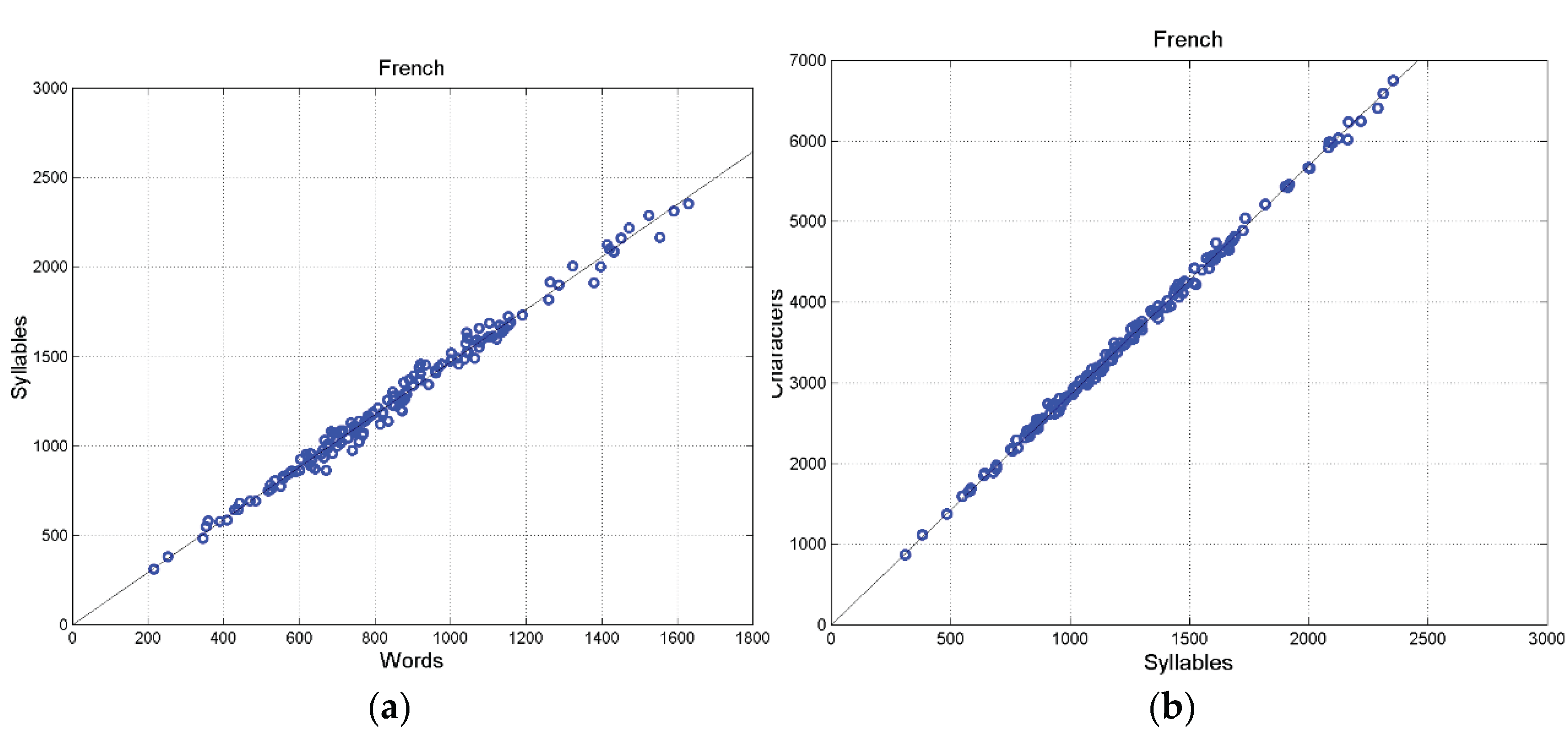
Figure A2.
German (a) Scatterplot between words and syllables; (b) scatterplot between characters and syllables (155 samples).
Figure A2.
German (a) Scatterplot between words and syllables; (b) scatterplot between characters and syllables (155 samples).
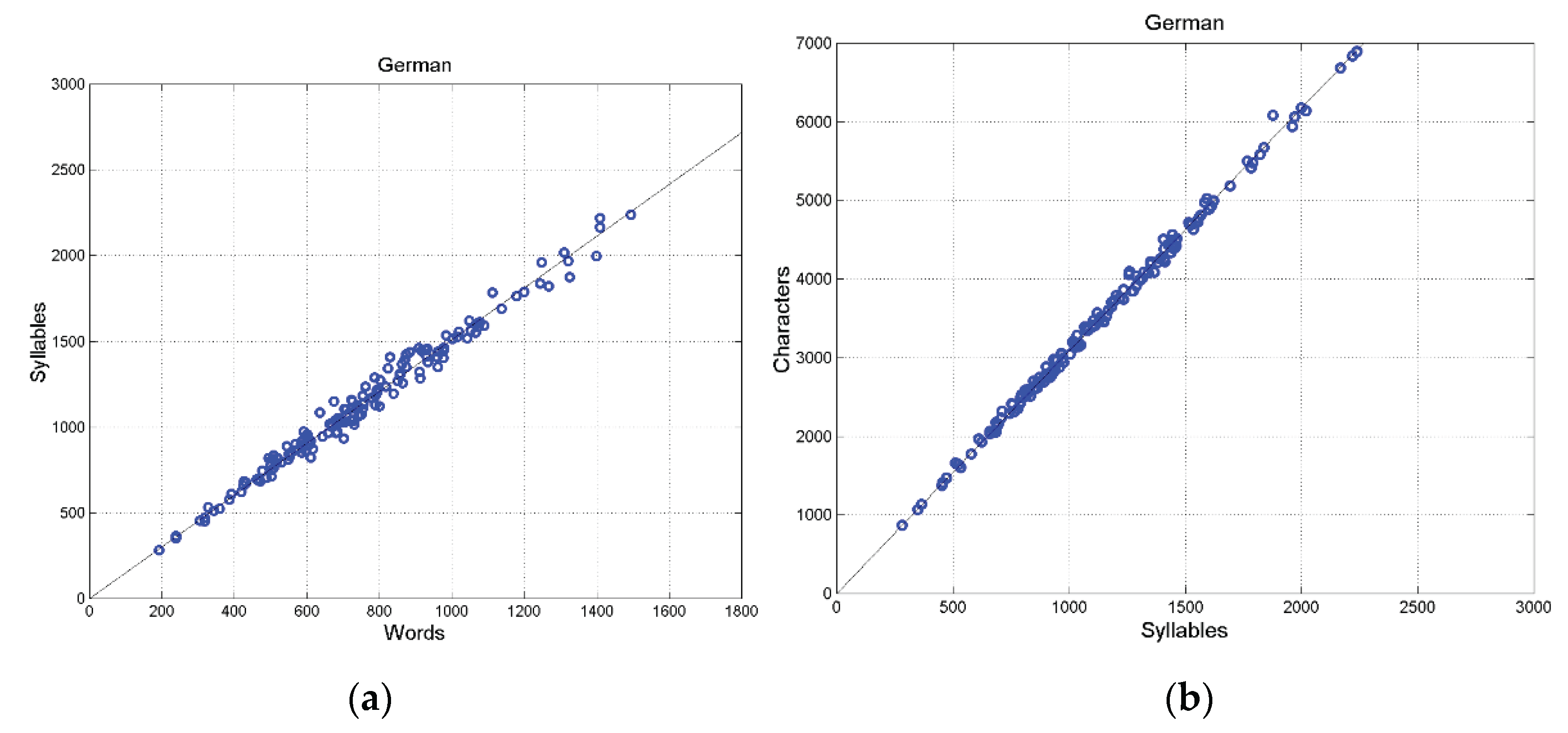
Figure A3.
Italian: (a) Scatterplot between words and syllables; (b) scatterplot between characters and syllables (155 samples).
Figure A3.
Italian: (a) Scatterplot between words and syllables; (b) scatterplot between characters and syllables (155 samples).
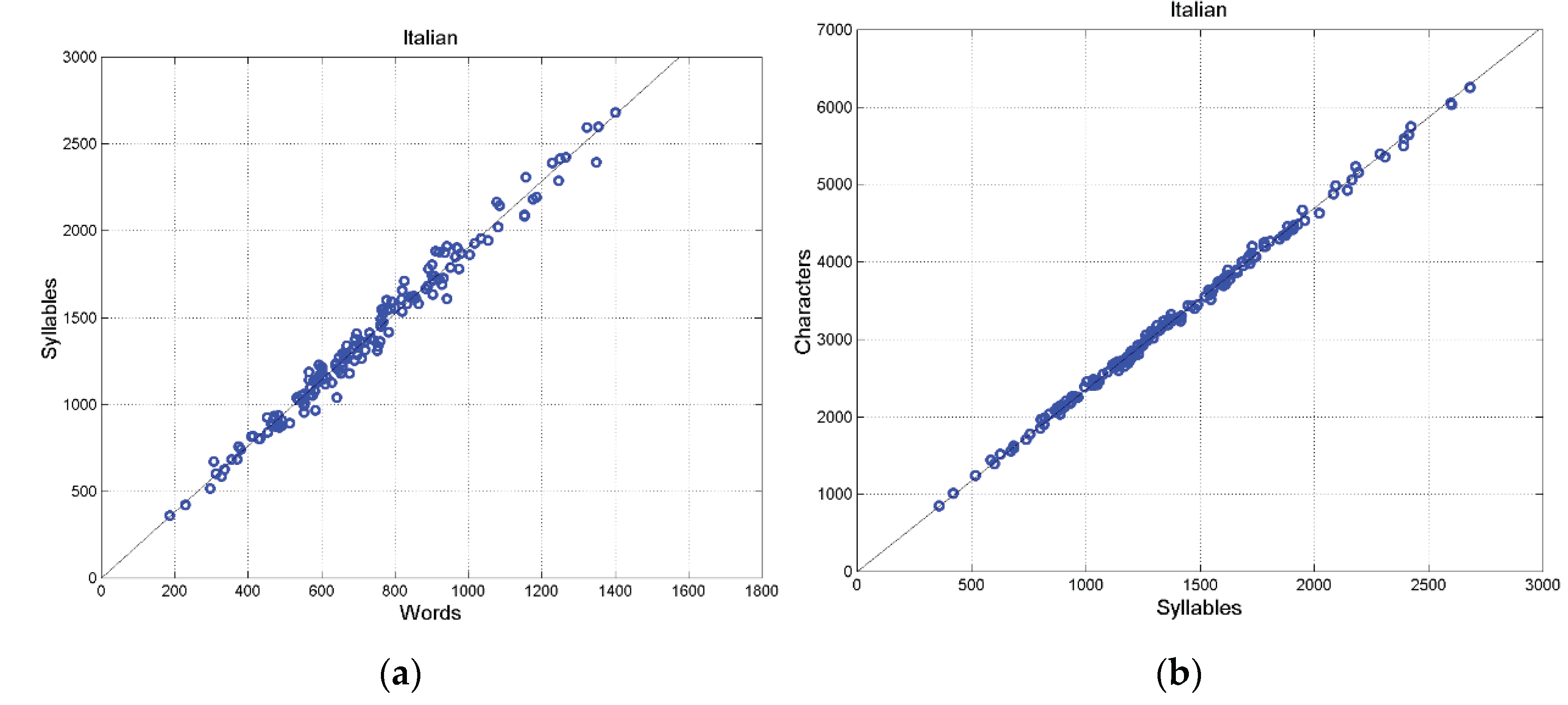
Figure A5.
Portuguese: (a) Scatterplot between words and syllables; (b) scatterplot between characters and syllables (155 samples).
Figure A6.
(a) French. Upper panel: Scatterplot between and words; Lower panel: scatterplot between and characters (155 samples). (b) German. Upper panel: Scatterplot between and words; Lower panel: scatterplot between and characters (155 samples). The mean value is drawn with the cyan line.
Figure A6.
(a) French. Upper panel: Scatterplot between and words; Lower panel: scatterplot between and characters (155 samples). (b) German. Upper panel: Scatterplot between and words; Lower panel: scatterplot between and characters (155 samples). The mean value is drawn with the cyan line.
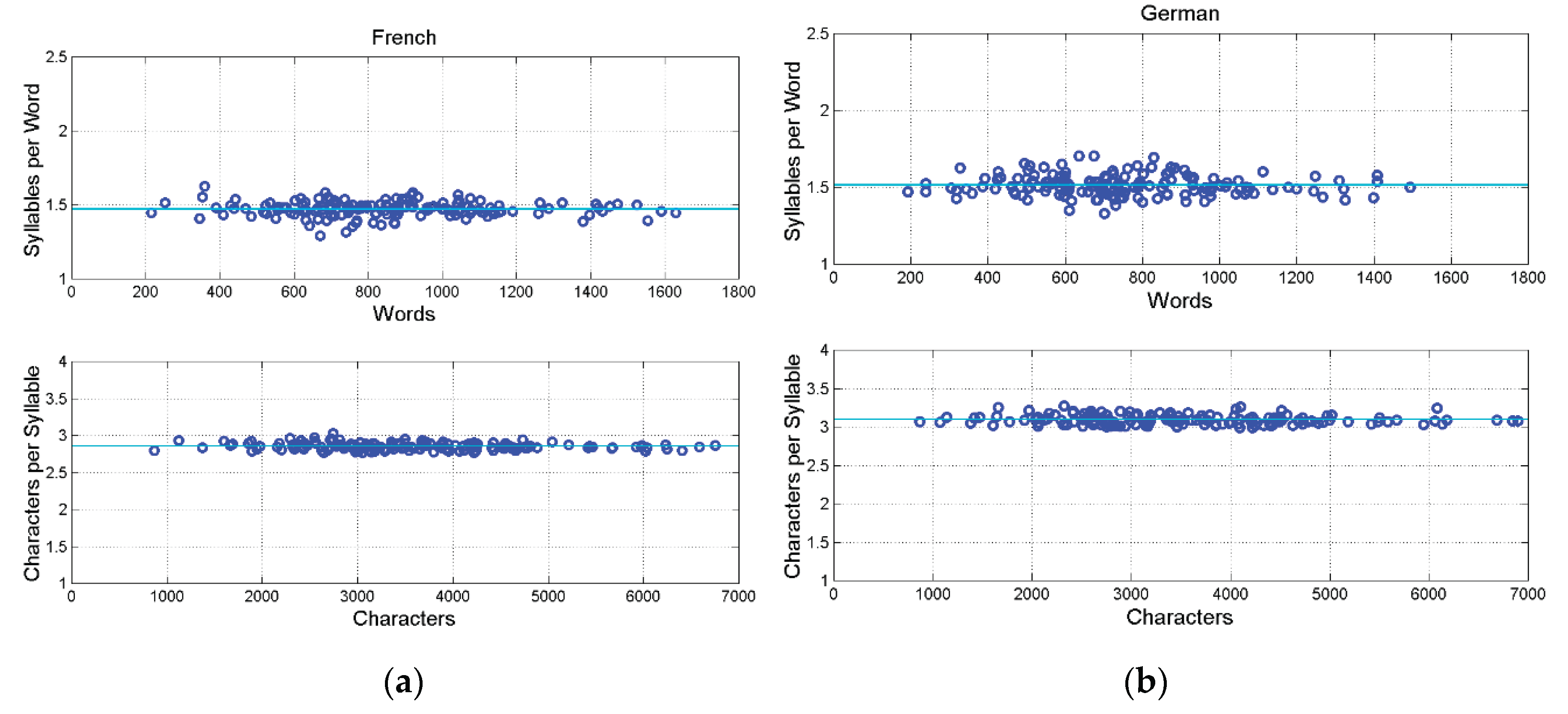
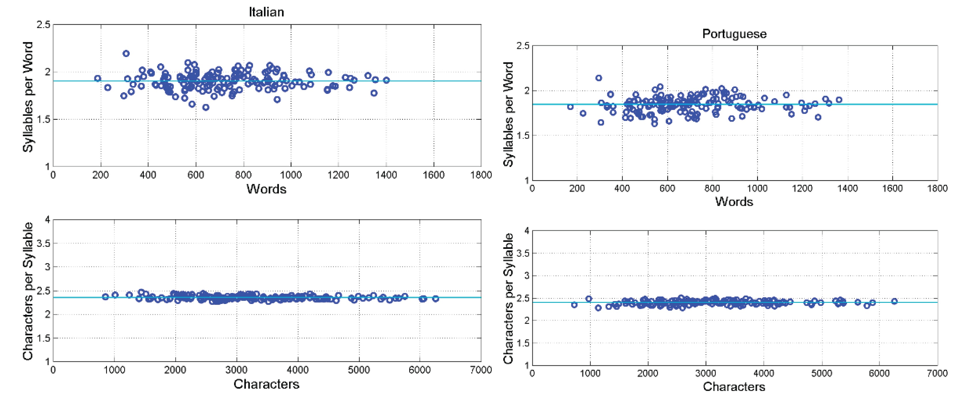
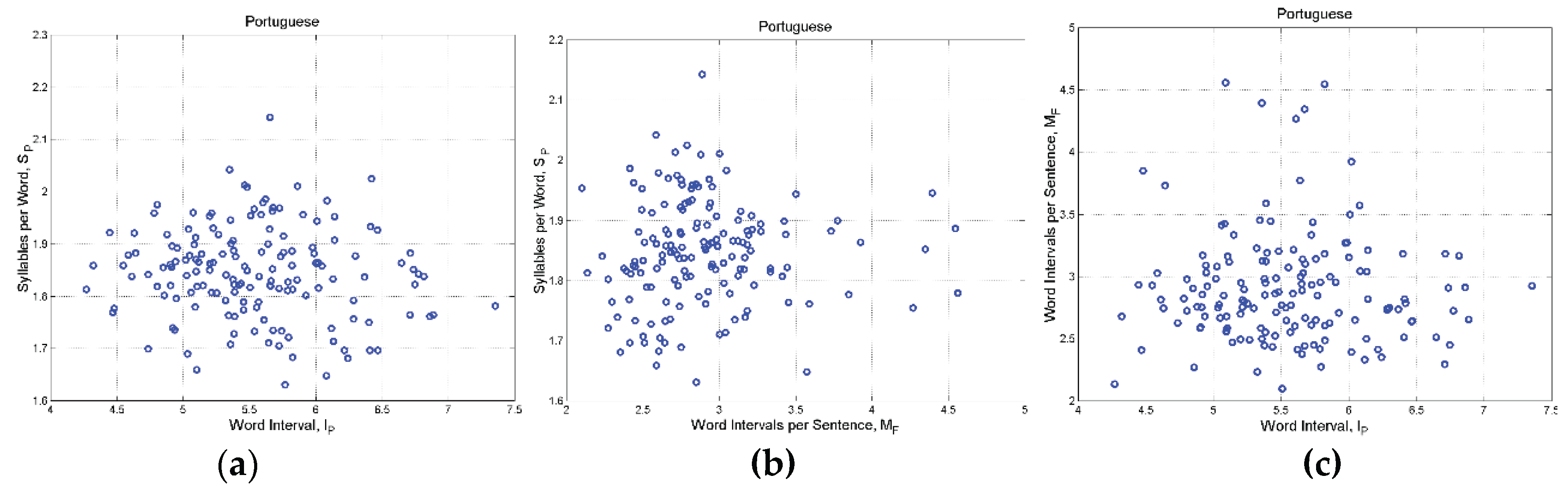
Figure A7.
(a) Italian. Upper panel: Scatterplot between and words; Lower panel: scatterplot between and characters (155 samples). (b) Portuguese. Upper panel: Scatterplot between and words; Lower panel: scatterplot between and characters (155 samples). The mean value is drawn with the cyan line.
Figure A7.
(a) Italian. Upper panel: Scatterplot between and words; Lower panel: scatterplot between and characters (155 samples). (b) Portuguese. Upper panel: Scatterplot between and words; Lower panel: scatterplot between and characters (155 samples). The mean value is drawn with the cyan line.
Appendix C. Unconditional Mean and Variance
Let and be the mean value and standard deviation of samples belonging to set , out of sets of the ensemble. From statistical theory [86,87,88], the unconditional mean (ensemble mean) is given by the mean of means:
The unconditional variance (ensemble variance) ( is the unconditional standard deviation) is given:
With
Appendix D. Three–Parameter Log−Normal Probability Density Modelling
Let us consider a stochastic variable (in linear units) with mean value and standard deviation (as those reported in Table 1).
Let us consider the variable linear transformation , with mean value and standard deviation , then the log−normal probability density function of is given by [86,87,88]:
where the mean (Np) and the standard deviation (Np) are given by:
Returning to the variable , its mode (most probable value) is given by:
The median (value exceeded with 0.5 probability) is given by:
Now, by assuming histogram bins centered at , with bin width , the number of samples per bin, out of total samples, is given by:
(A9)
In our case, , therefore we get the estimated histogram reported in Figure 4.
Appendix E. Correlation Coefficients Between Deep–Language Parameters
Table A1 reports the correlation coefficient between the logarithms of the indicated deep–language parameters, for each language. From this table we can conclude that and are practically uncorrelated. Because of the bivariate Gaussian modelling, they can be assumed to be independent.

Table A1.
Correlation coefficient between the logarithms of the indicated deep–language parameters, for each language.
Table A1.
Correlation coefficient between the logarithms of the indicated deep–language parameters, for each language.
| Language | |||||
|---|---|---|---|---|---|
| Greek | 0.3176 | –0.0988 | 0.0686 | –– | –– |
| Latin | 0.3568 | 0.0944 | 0.0157 | –– | –– |
| Esperanto | 0.0747 | 0.0680 | 0.2735 | –– | –– |
| French* | 0.1439 | –0.0643 | –0.3932 | 0.1403 | –0.0689 |
| Italian* | –0.0117 | 0.2950 | –0.2399 | –0.0785 | 0.2999 |
| Portuguese* | –0.2227 | –0.0814 | –0.0798 | –0.1029 | –0.0094 |
| Romanian° | –0.0366 | 0.4040 | –0.1230 | –– | –– |
| Spanish | 0.1052 | 0.1074 | –0.0320 | –– | –– |
| Danish° | 0.4588 | –0.2698 | –0.2699 | –– | –– |
| English* | 0.1568 | 0.3103 | –0.2650 | 0.0858 | 0.3320 |
| Finnish° | 0.2906 | 0.2024 | –0.1003 | –– | –– |
| German* | 0.2895 | 0.1232 | –0.3047 | 0.3531 | 0.0285 |
| Icelandic | 0.1487 | –0.0834 | –0.2382 | –– | –– |
| Norwegian° | 0.1708 | –0.1665 | –0.6105 | –– | –– |
| Swedish° | 0.2352 | –0.0189 | –0.6260 | –– | –– |
| Bulgarian | 0.2739 | –0.1167 | –0.2792 | –– | –– |
| Czech° | 0.1935 | 0.0708 | –0.1467 | –– | –– |
| Croatian° | 0.1446 | 0.1111 | 0.0007 | –– | –– |
| Polish° | 0.2423 | –0.0994 | –0.2518 | –– | –– |
| Russian | 0.0686 | 0.1369 | 0.0508 | –– | –– |
| Serbian | 0.0424 | 0.2215 | –0.2461 | –– | –– |
| Slovak | 0.2195 | –0.0266 | –0.2101 | –– | –– |
| Ukrainian | 0.3878 | –0.3976 | –0.5274 | –– | –– |
| Estonian° | 0.3783 | 0.1358 | –0.1090 | –– | –– |
| Hungarian° | 0.2464 | –0.2439 | –0.0263 | –– | –– |
| Albanian | –0.0244 | 0.1433 | 0.0388 | –– | –– |
| Armenian | 0.2587 | 0.2234 | 0.1047 | –– | –– |
| Welsh | –0.0800 | 0.0988 | –0.0313 | –– | –– |
| Basque | 0.2283 | –0.0678 | –0.0450 | –– | –– |
| Hebrew | 0.2078 | 0.2880 | –0.1593 | –– | –– |
| Cebuano | 0.1130 | –0.2173 | –0.5899 | –– | –– |
| Tagalog | 0.2838 | –0.3915 | –0.3069 | –– | –– |
| Chichewa | –0.0003 | –0.0935 | –0.4157 | –– | –– |
| Luganda | –0.0569 | 0.1538 | –0.1771 | –– | –– |
| Somali | –0.0243 | –0.1853 | 0.1491 | –– | –– |
| Haitian | 0.2753 | 0.0173 | –0.3800 | –– | –– |
| Nahuatl | –0.2043 | –0.0967 | –0.5228 | –– | –– |
Appendix F. Scatterplots Between
Figure A8, Figure A9, Figure A10, Figure A11 and Figure A12 show the scatterplots between (or and for the indicated languages.
Figure A8.
Latin: (a) Scatterplot between and ; (b) Scatterplot between and . (c) Scatterplot between and .
Figure A8.
Latin: (a) Scatterplot between and ; (b) Scatterplot between and . (c) Scatterplot between and .
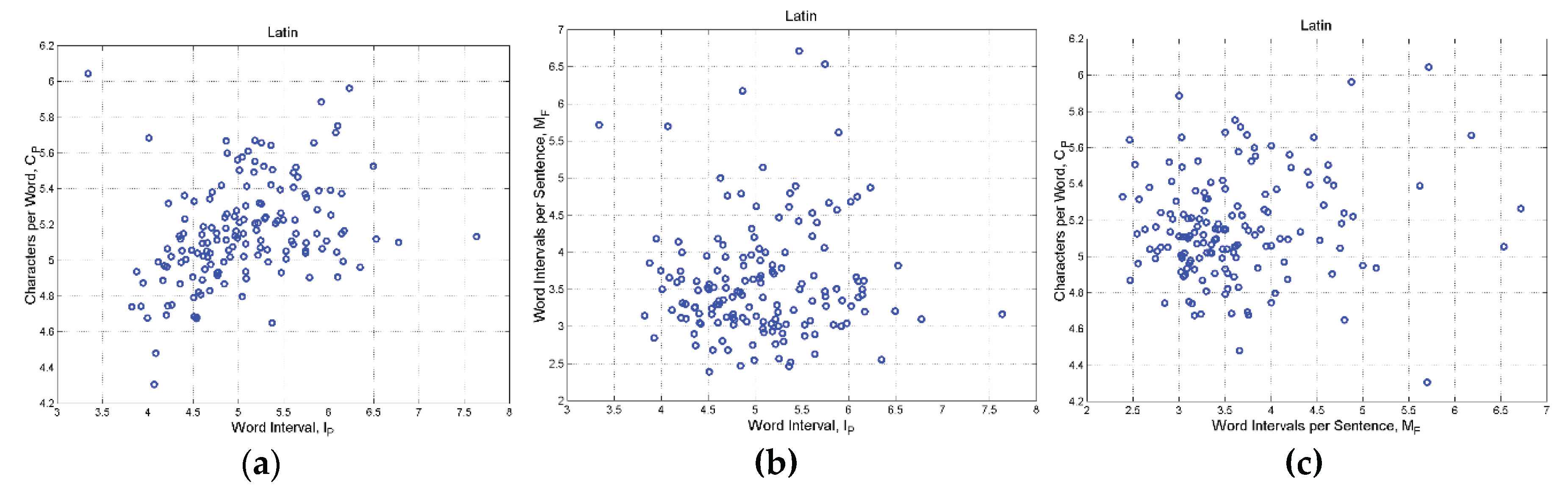
Figure A9.
French: (a) Scatterplot between
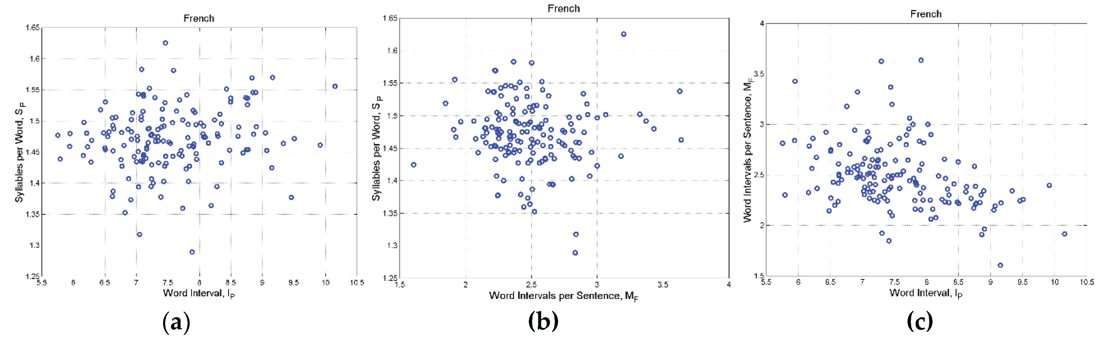
Figure A10.
German: (a) Scatterplot between and ; (b) Scatterplot between and ; (c) Scatterplot between and .
Figure A10.
German: (a) Scatterplot between and ; (b) Scatterplot between and ; (c) Scatterplot between and .
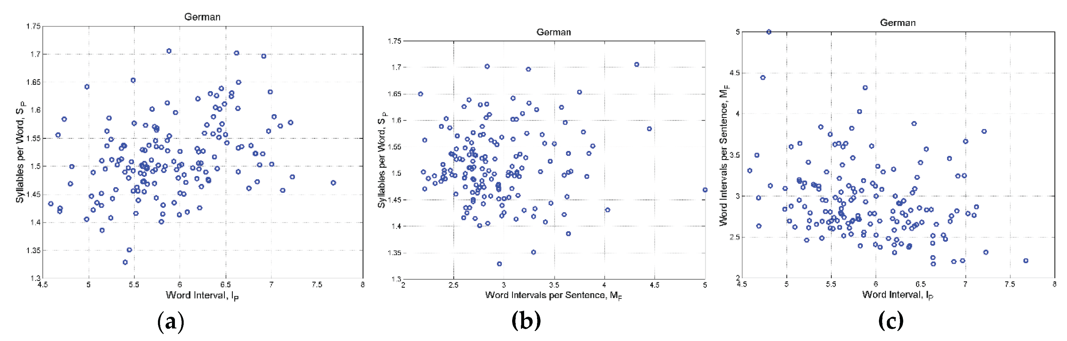
Figure A11.
Italian: (a) Scatterplot between
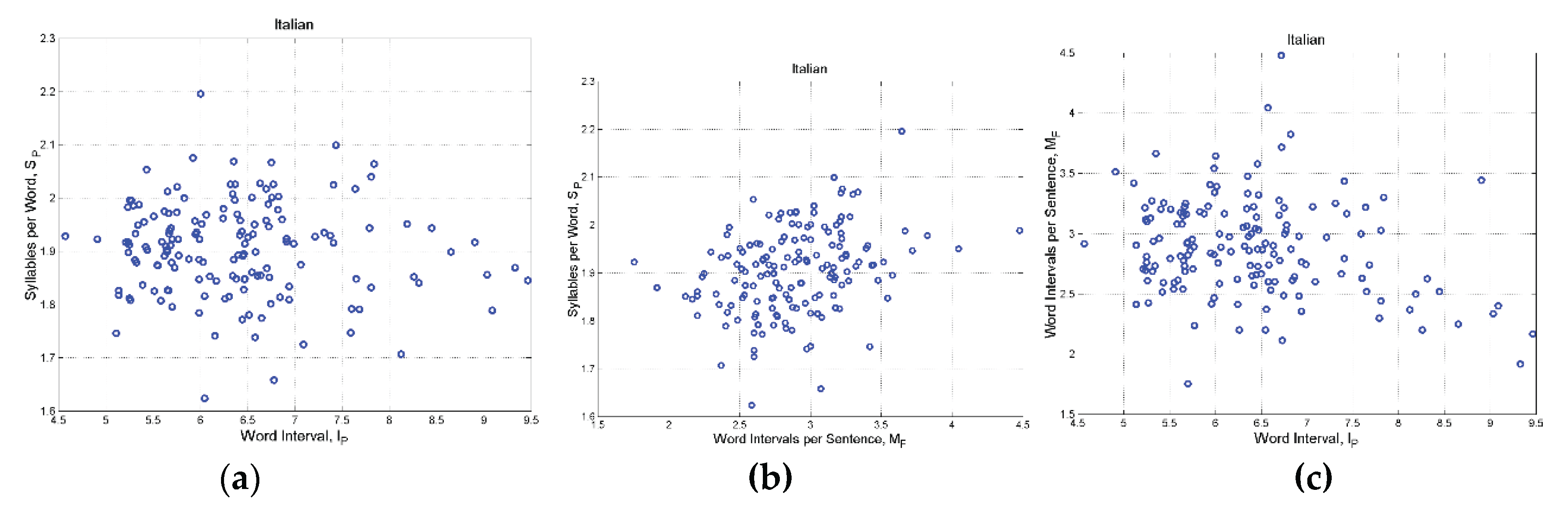
Figure A12.
Portuguese: (a) Scatterplot between
References
- Deniz, F.; Nunez–Elizalde, A.O.; Huth, A.G.; Gallant Jack, L. The Representation of Semantic Information Across Human Cerebral Cortex During Listening Versus Reading Is Invariant to Stimulus Modality 2019, J. Neuroscience, 39, 7722–7736.
- Matricciani, E. A Mathematical Structure Underlying Sentences and Its Connection with Short–Term Memory. AppliedMath 2024, 4, 120–142. [Google Scholar] [CrossRef]
- Matricciani, E. Is Short–Term Memory Made of Two Processing Units? Clues from Italian and English Literatures down Several Centuries. Information 2024, 15, 6. [Google Scholar] [CrossRef]
- Matricciani, E. Deep Language Statistics of Italian throughout Seven Centuries of Literature and Empirical Connections with Miller’s 7 ∓ 2 Law and Short–Term Memory. Open Journal of Statistics 2019, 9, 373–406. [Google Scholar] [CrossRef]
- Matricciani, E. Linguistic Mathematical Relationships Saved or Lost in Translating Texts: Extension of the Statistical Theory of Translation and Its Application to the New Testament. Information 2022, 13, 20. [Google Scholar] [CrossRef]
- Matricciani, E. (2023) Short–Term Memory Capacity across Time and Language Estimated from Ancient and Modern Literary Texts. Study–Case: New Testament Translations. Open Journal of Statistics, 13, 379–403. [CrossRef]
- Matricciani, E. Capacity of Linguistic Communication Channels in Literary Texts: Application to Charles Dickens’ Novels. Information 2023, 14, 68. [Google Scholar] [CrossRef]
- Matricciani, E. Linguistic Communication Channels Reveal Connections between Texts: The New Testament and Greek Literature. Information 2023, 14, 405. [Google Scholar] [CrossRef]
- Matricciani, E. Multi–Dimensional Data Analysis of Deep Language in J.R.R. Tolkien and C.S. Lewis Reveals Tight Mathematical Connections. AppliedMath 2024, 4, 927–949. [Google Scholar] [CrossRef]
- Matricciani, E. (2025) A Mathematical Analysis of Texts of Greek Classical Literature and Their Connections. Open Journal of Statistics, 15, 1–34. [CrossRef]
- Miller, G.A. The Magical Number Seven, Plus or Minus Two. Some Limits on Our Capacity for Processing Information, 1955, Psychological Review, 343−352.
- Crowder, R.G. Short–term memory: Where do we stand?, 1993, Memory & Cognition, 21, 142–145.
- Lisman, J.E. , Idiart, M.A.P. Storage of 7 ± 2 Short–Term Memories in Oscillatory Subcycles, 1995, Science, 267, 5203,. 1512– 1515.
- Cowan, N. , The magical number 4 in short−term memory: A reconsideration of mental storage capacity, Behavioral and Brain Sciences, 2000, 87−114.
- Bachelder, B.L. The Magical number 7± 2 span Theory on Capacity Limitations. Behavioral and Brain Sciences 2001, 24, 116–117. [Google Scholar] [CrossRef]
- Saaty, T.L. , Ozdemir, M.S., Why the Magic Number Seven Plus or Minus Two, Mathematical and Computer Modelling, 2003, 233−244.
- Burgess, N. , Hitch, G.J. A revised model of short–term memory and long–term learning of verbal sequences, 2006, Journal of Memory and Language, 55, 627–652.
- Richardson, J.T. E, Measures of short–term memory: A historical review, 2007, Cortex, 43, 5, 635–650.
- Mathy, F. , Feldman, J. What’s magic about magic numbers? Chunking and data compression in short−term memory, Cognition, 2012, 346−362.
- Gignac, G.E. The Magical Numbers 7 and 4 Are Resistant to the Flynn Effect: No Evidence for Increases in Forward or Backward Recall across 85 Years of Data. Intelligence, 2015, 48, 85–95. [Google Scholar] [CrossRef]
- Trauzettel−Klosinski, S., K. Dietz, K. Standardized Assessment of Reading Performance: The New International Reading Speed Texts IreST, IOVS 2012, 5452−5461.
- Melton, A.W. , Implications of Short–Term Memory for a General Theory of Memory, 1963, Journal of Verbal Learning and Verbal Behavior, 2, 1–21.
- Atkinson, R.C. , Shiffrin, R.M., The Control of Short–Term Memory, 1971, Scientific American, 225, 2, 82–91.
- Murdock, B.B. Short–Term Memory, 1972, Psychology of Learning and Motivation, 5, 67–127.
- Baddeley, A.D. , Thomson, N. , Buchanan, M., Word Length and the Structure of Short−Term Memory, Journal of Verbal Learning and Verbal Behavior, 1975, 14, 575−589. [Google Scholar]
- Case, R. , Midian Kurland, D., Goldberg, J. Operational efficiency and the growth of short–term memory span, 1982, Journal of Experimental Child Psychology, 33, 386–404.
- Grondin, S. A temporal account of the limited processing capacity, Behavioral and Brain Sciences, 2000, 24, 122−123.
- Pothos, E.M. , Joula, P., Linguistic structure and short−term memory, Behavioral and Brain Sciences, 2000, 138−139.
- Conway, A.R.A., Cowan, N., Michael F. Bunting, M.F., Therriaulta, D.J., Minkoff, S.R.B., A latent variable analysis of working memory capacity, short−term memory capacity, processing speed, and general fluid intelligence, Intelligence, 2002, 163−183.
- Jonides, J. , Lewis, R.L., Nee, D.E., Lustig, C.A., Berman, M.G., Moore, K.S., The Mind and Brain of Short–Term Memory, 2008 Annual Review of Psychology, 69, 193–224.
- Barrouillest, P. , Camos, V., As Time Goes By: Temporal Constraints in Working Memory, Current Directions in Psychological Science, 2012, 413−419.
- Potter, M.C. Conceptual short term memory in perception and thought, 2012, Frontiers in Psychology. [CrossRef]
- Jones, G, Macken, B., Questioning short−term memory and its measurements: Why digit span measures long−term associative learning, Cognition, 2015, 1−13.
- Chekaf, M. , Cowan, N. , Mathy, F., Chunk formation in immediate memory and how it relates to data compression, Cognition, 2016, 155, 96−107. [Google Scholar]
- Norris, D. , Short–Term Memory and Long–Term Memory Are Still Different, 2017, Psychological Bulletin, 143, 9, 992–1009.
- Houdt, G.V. , Mosquera, C., Napoles, G., A review on the long short–term memory model, 2020, Artificial Intelligence Review, 53, 5929–5955.
- Islam, M., Sarkar, A., Hossain, M., Ahmed, M., Ferdous, A. Prediction of Attention and Short–Term Memory Loss by EEG Workload Estimation. Journal of Biosciences and Medicines, 2023, 304–31. [CrossRef]
- Rosenzweig, M.R. , Bennett, E. L., Colombo, P.J., Lee, P.D.W. Short–term, intermediate–term and Long–term memories,, Behavioral Brain Research, 1993, 57, 2, 193–198. [Google Scholar]
- Kaminski, J. Intermediate–Term Memory as a Bridge between Working and Long–Term Memory, The Journal of Neuroscience, 2017, 37(20), 5045–5047.
- Strinati E., C. , Barbarossa S. 6G Networks: Beyond Shannon Towards Semantic and Goal–Oriented Communications, 2021, Computer Networks, 190, 8, 1–17.
- Shi, G. , Xiao, Y, Li, Xie, X. From semantic communication to semantic–aware networking: Model, architecture, and open problems, 2021, IEEE Communications Magazine, 59, 8, 44–50.
- Xie, H. , Qin, Z., Li, G.Y., Juang, B.H. Deep learning enabled semantic communication systems, 2021, IEEE Trans. Signal Processing, 69, 2663–2675.
- Luo, X. , Chen, H.H., Guo, Q. Semantic communications: Overview, open issues, and future research directions, 2022, IEEE Wireless Communications, 29, 1, 210–219.
- Wanting, Y. , Hongyang, D, Liew, Z. Q., Lim, W.Y.B., Xiong, Z., Niyato, D., Chi, X., Shen, X., Miao, C. Semantic Communications for Future Internet: Fundamentals, Applications, and Challenges, 2023, IEEE Communications Surveys & Tutorials, 25, 1, 213–250.
- Xie, H. , Qin, Z., Li, G.Y., Juang, B.H. Deep learning enabled semantic communication systems, 2021, IEEE Trans. Signal Processing, 69, 2663–2675.
- Bellegarda, J.R. , Exploiting Latent Semantic Information in Statistical Language Modeling, 2000, Proceedings of the IEEE, 88, 8, 1279–1296.
- D’Alfonso, S., On Quantifying Semantic Information, 2011, Information, 2, 61–101. [CrossRef]
- Zhong, Y. , A Theory of Semantic Information, 2017, China Communications, 1–17.
- Levelt, W. J. M. , Roelofs, A., Meyer, A. S., A Theory of Lexical Access in Speech Production. 1999, Cambridge Univ. Press, 1999.
- Kazanina, N. , Bowers, J. S. & Idsardi, W. Phonemes: lexical access and beyond. 2018. Psychon. Bull. Rev. 25, 560–585.
- Khanna, A.R., Muñoz, W., Joon Kim, Y.J, Kfir, Y., Paulk, A.C., Jamali, M., Cai, J., Mustroph, M.L., Caprara, I., Hardstone, R., Mejdell, M., Meszéna, D., Zuckerman, A., Schweitzer, J., Cash, S., Williams, Z.M. Single–neuronal elements of speech production in humans. 2024. Nature, 626, 603–610. [CrossRef]
- Bohland, J. W., Guenther, F. H. An fMRI investigation of syllable sequence production. 2006. NeuroImage 32, 821–841.
- Basilakos, A., Smith, K. G., Fillmore, P., Fridriksson, J., Fedorenko, E. Functional characterization of the human speech articulation network. 2017. Cereb. Cortex 28, 1816–1830.
- Lee, D. K., Fedorenko, E., Simon, M.V., Curry, W.T., Nahed, B.V., Cahill, D.P., Williams, Z.M. Neural encoding and production of functional morphemes in the posterior temporal lobe. 2018. Nat. Commun. 9, 1877.
- Glanz, O., Hader, M., Schulze–Bonhage, A., Auer, P., Ball, T. A study of word complexity under conditions of non–experimental, natural overt speech production using ECoG. Front. 2021. Hum. Neurosci. 15. [CrossRef]
- Fedorenko, E. , Scott, T.L., Brunner, P., Kanwisher, N. Neural correlate of the construction of sentence meaning. 2016. Proc. Natl Acad. Sci. USA 113, E6256–E6262.
- Nelson, M. J., Karoui , I.E., Giber , K., Yang , X., Cohen, L., Koopman, H., Cash, S.S., Naccache, L., Hale, J.T., Pallier, C., Dehaene, S. Neurophysiological dynamics of phrase–structure building during sentence processing. 2017. Proc. Natl Acad. Sci. USA 114, E3669–E3678.
- Walenski, M. , Europa, E., Caplan, D., Thompson, C. K. Neural networks for sentence comprehension and production: an ALE–based meta–analysis of neuroimaging studies. 2019. Hum. Brain Mapp. 40, 2275–2304.
- Rosen, S. Temporal information in speech: Acoustic, auditory and linguistic aspects. 1992. Philos. Trans. R. Soc. Lond. B Biol. Sci. 336, 367–373.
- Poeppel, D., The analysis of speech in different temporal integration windows: cerebral lateralization as ‘asymmetric sampling in time’. 2003. Speech Commun. 41, 245–255.
- Saberi, K. , Perrott, D. R. Cognitive restoration of reversed speech. 1999, Nature 398, 760. [Google Scholar]
- Giraud, D. Poeppel, cortical oscillations and speech processing: emerging computational principles and operations. 2012. Nat. Neurosci. 15, 511–517.
- Ghitza, O. Linking speech perception and neurophysiology: Speech decoding guided by cascaded oscillators locked to the input rhythm. 2011. Front. Psychol.
- Doelling, K.B. , Arnal, L.H., Ghitza, O., Poeppel, D. Acoustic landmarks drive delta– theta oscillations to enable speech comprehension by facilitating perceptual parsing. 2014. Neuroimage.
- Peelle, J. E., Gross, J., Davis, M.H. Phase– locked responses to speech in human auditory cortex are enhanced during comprehension. 2013. Cereb. Cortex 23, 1378–1387.
- Luo, H. , Poeppel, D. Phase patterns of neuronal responses reliably discriminate speech in human auditory cortex. 2007. Neuron 54, 1001–1010.
- Park, H., R., Ince, R.A.A., Schyns, P.G., Thut, G., Gross, J. Frontal top– down signals increase coupling of auditory low– frequency oscillations to continuous speech in human listeners. 2023. Curr. Biol. 25, 1649–1653.
- Oganian, Y., Chang, F. A speech envelope landmark for syllable encoding in human superior temporal gyrus. 2019. Sci. Adv. 5, eaay6279.
- Giroud, J., Lerousseau, J.P., Pellegrino, F., Morillon, B. The channel capacity of multilevel linguistic features constrains speech comprehension. 2023. Cognition 232, 105345.
- Poeppel, D., Assaneo, M.F. Speech rhythms and their neural foundations. 2020. Nat. Rev. Neurosci. 21, 322–334.
- Keitel, A., Gross, J., Kayser, C., Perceptually relevant speech tracking in auditory and motor cortex reflects distinct linguistic features. 2018. PLOS Biol. 16, e2004473.
- Ding, N., Simon, J.Z. Cortical entrainment to continuous speech: Functional roles and interpretations. 2014. Front. Hum. Neurosci. 8, 311.
- Lubinus, C. , Keitel, A., Obleser, J., Poeppel, D., Rimmele, J.M. Explaining flexible continuous speech comprehension from individual motor rhythms. 2023. Proc. Biol. Sci, 2022. [Google Scholar]
- Carreiras, M. , Álvarez, C. J., Devega, M. Syllable frequency and visual word recognition in Spanish. 1993, 32(6), 766–780. [Google Scholar]
- Ferrand, L. , Segui, J., Grainger, J. Masked priming of word and picture naming: The role of syllabic units. 1996. Journal of Memory and Language, 35(5), 708–723.
- Ferrand, L., Segui, J., Humphreys, G. W. The syllable’s role in word naming. 1997. Memory & Cognition, 25(4), 458–470.
- Lundmark, M.S. , Erickson, D., Segmental and Syllabic Articulations: A Descriptive Approach, Journal of Speech, Language, and Hearing Research. 2022. 67, 3974–4001.
- Matricciani, E. A Statistical Theory of Language Translation Based on Communication Theory. Open J. Stat. 2020, 10, 936–997. [Google Scholar] [CrossRef]
- Matricciani, E. Readability Indices Do Not Say It All on a Text Readability. Analytics 2023, 2, 296–314. [Google Scholar] [CrossRef]
- Matricciani, E. Readability across Time and Languages: The Case of Matthew’s Gospel Translations. AppliedMath 2023, 3, 497–509. [Google Scholar] [CrossRef]
- Parkes, Malcolm B. Pause and Effect. An Introduction to the History of Punctuation in the West, 2016, Abingdon, Routledge.
- Matricciani, E. Translation Can Distort the Linguistic Parameters of Source Texts Written in Inflected Language: Multidimensional Mathematical Analysis of “The Betrothed”, a Translation in English of “I Promessi Sposi” by A. Manzoni. AppliedMath 2025, 5, 24. [Google Scholar] [CrossRef]
- Matricciani, E. Domestication of Source Text in Literary Translation Prevails over Foreignization. Analytics 2025, 4, 17. [Google Scholar] [CrossRef]
- Flesch, R. , The Art of Readable Writings. 1974. Harper and Row, New York, Revised and Enlarged 25th anniversary edition.
- Matricciani, E. Readability Indices Do Not Say It All on a Text Readability. Analytics 2023, 2, 296–314. [Google Scholar] [CrossRef]
- Papoulis Papoulis, A. Probability & Statistics; Prentice Hall: Hoboken, NJ, USA, 1990. [Google Scholar]
- Lindgren, B.W. Statistical Theory, 2nd ed.; 1968, MacMillan Company: New York, NY, USA.
- Bury, K.V. Statistical Models in Applied Science, 1975, John Wiley.
- Flesch, R. , A New Readability Yardstick, Journal of Applied Psychology, 1948, 222–233.
- Flesch, R. , The Art of Readable Writing, Harper & Row, New York, revised and enlarged edition, 1974.
- Kincaid, J.P. , Fishburne, R.P, Rogers, R.L., Chissom, B.S., Derivation Of New Readability Formulas (Automated Readability Index, Fog Count And Flesch Reading Ease Formula) For Navy Enlisted Personnel, 1975, Research Branch Report 8–75, Chief of Naval Technical Training. Naval Air Station, Memphis, TN, USA.
- DuBay, W.H. , The Principles of Readability, 2004, Impact Information, Costa Mesa, California.
- Bailin, A. , Graftstein, A. The linguistic assumptions underlying readability formulae: a critique, Language & Communication, 2001, 21, 285−301. [Google Scholar]
- DuBay (Editor), W.H. , The Classic Readability Studies, 2006, Impact Information, Costa Mesa, California.
- Zamanian, M. , Heydari, P., Readability of Texts: State of the Art, Theory and Practice in Language Studies, 2012, 43−53.
- Benjamin, R.G. Reconstructing Readability: Recent Developments and Recommendations in the Analysis of Text Difficulty, Educ Psycological Review, 2012, 63−88.
- Collins−Thompson, K. , Computational Assessment of Text Readability: A Survey of Past, in Present and Future Research, Recent Advances in Automatic Readability Assessment and Text Simplification, ITL, International Journal of Applied Linguistics, 2014, 97−135.
- Kandel, L.; Moles, A.; Application de l’indice de Flesch à la langue française. Cahiers Etudes de Radio–Télévision, 1958, 253–274.
- François, T. ; An analysis of a French as Foreign language corpus for readability assessment. Proceedings of the 3rd workshop on NLP for CALL, 2014; 22. [Google Scholar]
- Lucisano, P., Piemontese, M.E., GULPEASE: una formula per la predizione della difficoltà dei testi in lingua italiana, Scuola e città, 1988, 110−124.
Figure 1.
Flow–chart of three processing units (processors) of human STM. Syllables , ,… are stored in the first processor, from 1 to about items, until a space or an interpunction is introduced (vertical arrow) to fix the length of the word. Words , ,… are stored in the second processor – approximately in Miller’s range – until an interpunction (vertical arrow) is introduced to fix the length of . The word interval is then stored in the third processor, from about 1 to 6 items, until the sentence ends with a full stop, a question mark or an exclamation mark (vertical arrow). The process is then repeated for the next sentence.
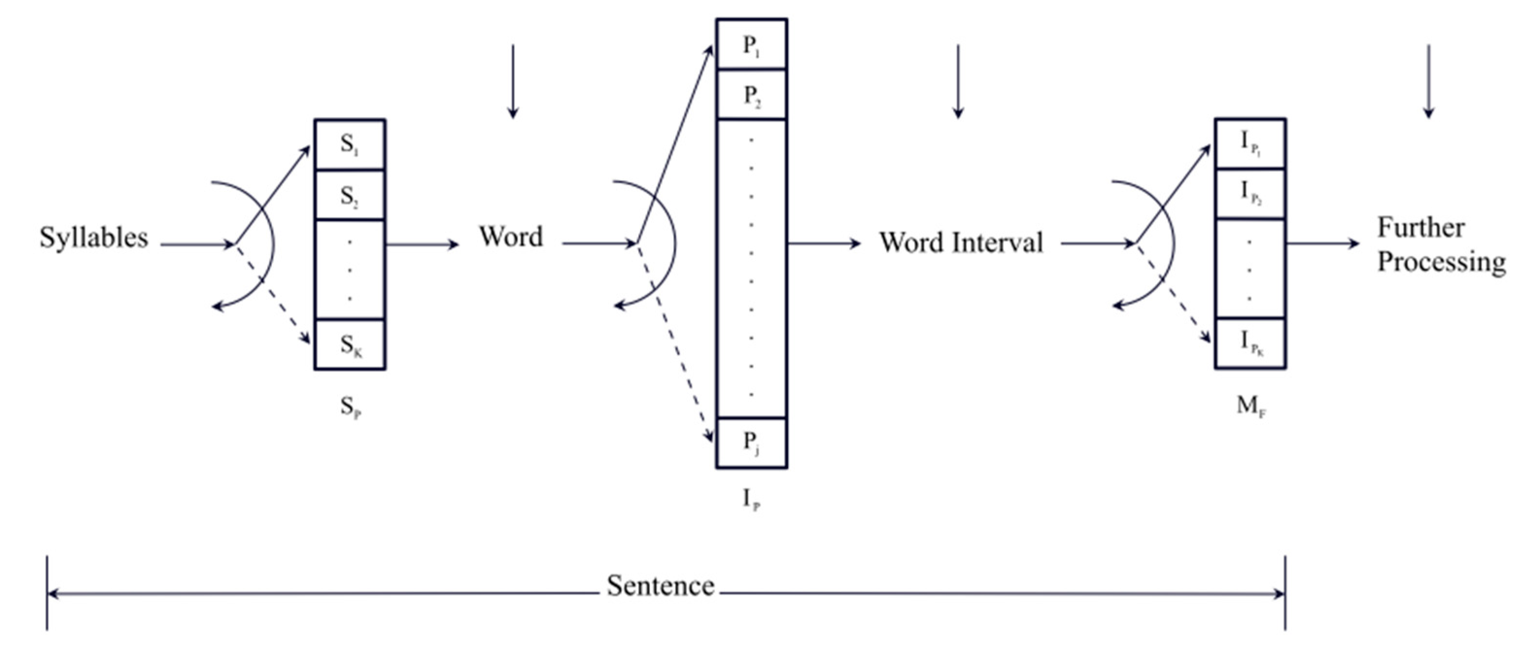
Figure 2.
English: (a) Scatterplot between words and syllables; (b) scatterplot between characters and syllables (155 samples).
Figure 2.
English: (a) Scatterplot between words and syllables; (b) scatterplot between characters and syllables (155 samples).
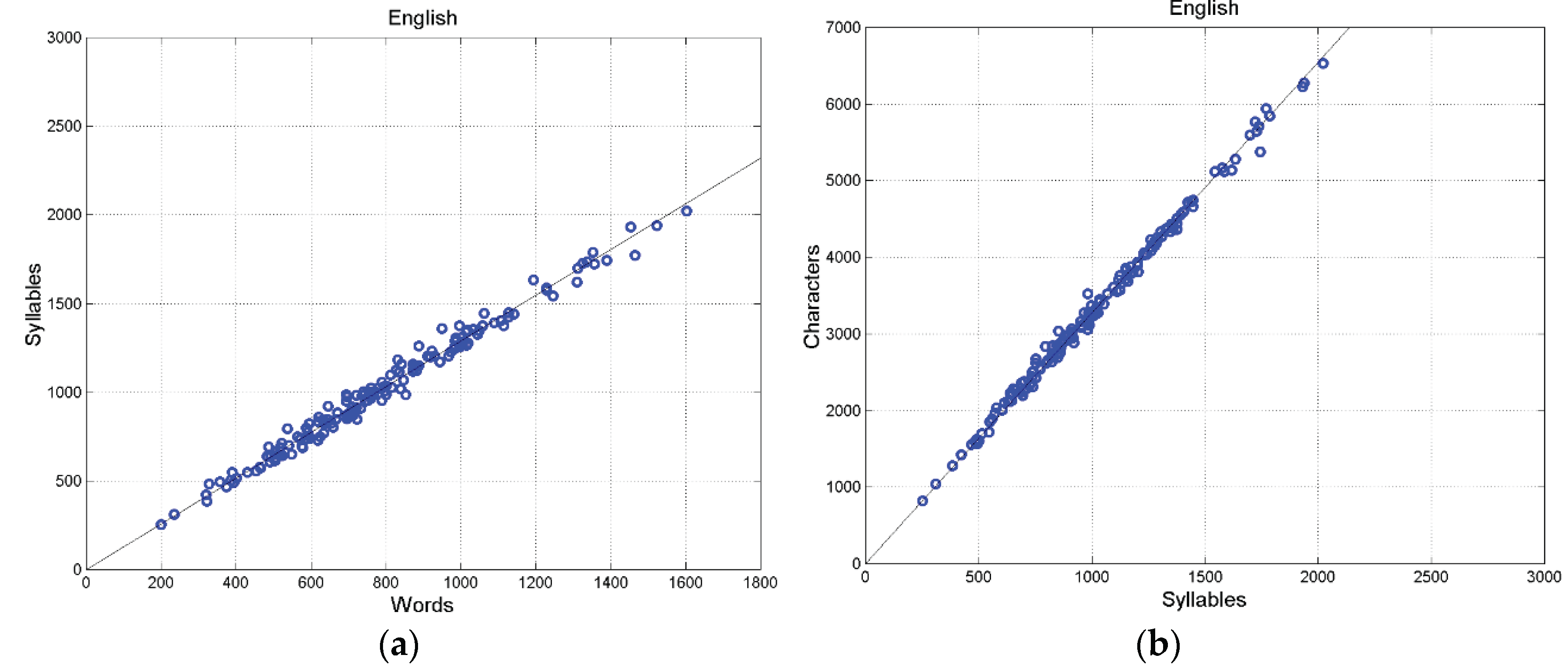
Figure 3.
English: Upper panel: Scatterplot between and words; Lower panel: scatterplot between and characters (155 samples). The mean value is drawn with the cyan line.
Figure 3.
English: Upper panel: Scatterplot between and words; Lower panel: scatterplot between and characters (155 samples). The mean value is drawn with the cyan line.
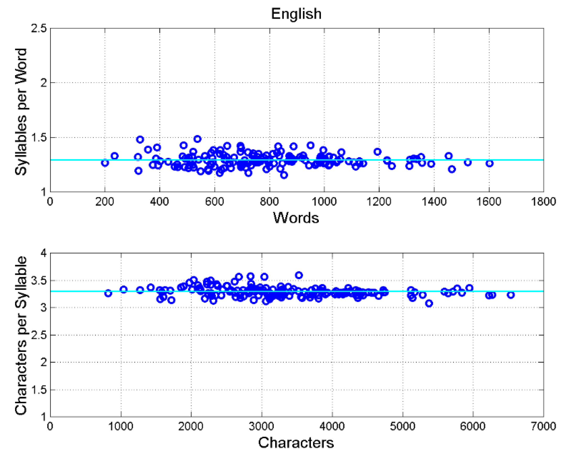
Figure 4.
Flow–chart of the first STM processor linking syllables to characters. The multiplying factor is given in Table 3 for some languages..
Figure 4.
Flow–chart of the first STM processor linking syllables to characters. The multiplying factor is given in Table 3 for some languages..
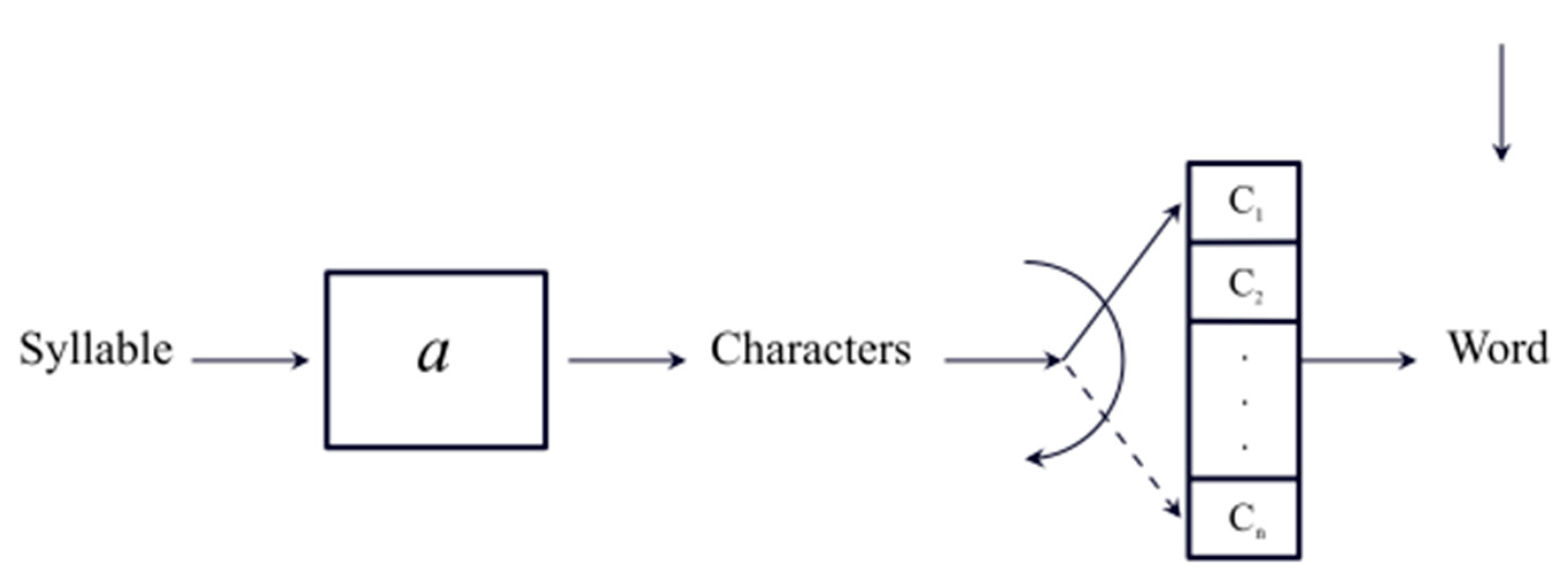
Figure 5.
Histogram of and three–parameter lognormal model, pooled data of Italian and Portuguese ( samples).
Figure 5.
Histogram of and three–parameter lognormal model, pooled data of Italian and Portuguese ( samples).
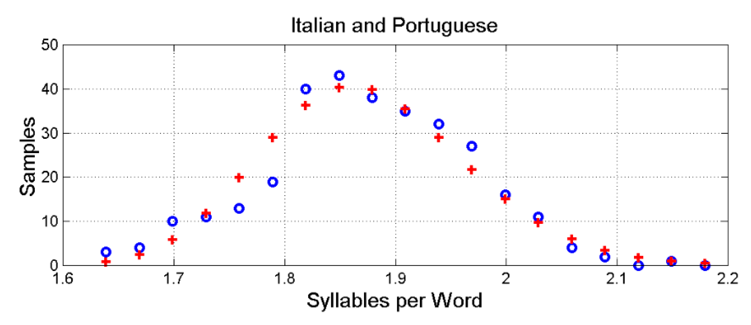
Figure 6.
English: (a) Scatterplot between and , correlation coefficient between the logarithms of the variables is ; (b) Scatterplot between and , ; (c) Scatterplot between and , .
Figure 6.
English: (a) Scatterplot between and , correlation coefficient between the logarithms of the variables is ; (b) Scatterplot between and , ; (c) Scatterplot between and , .
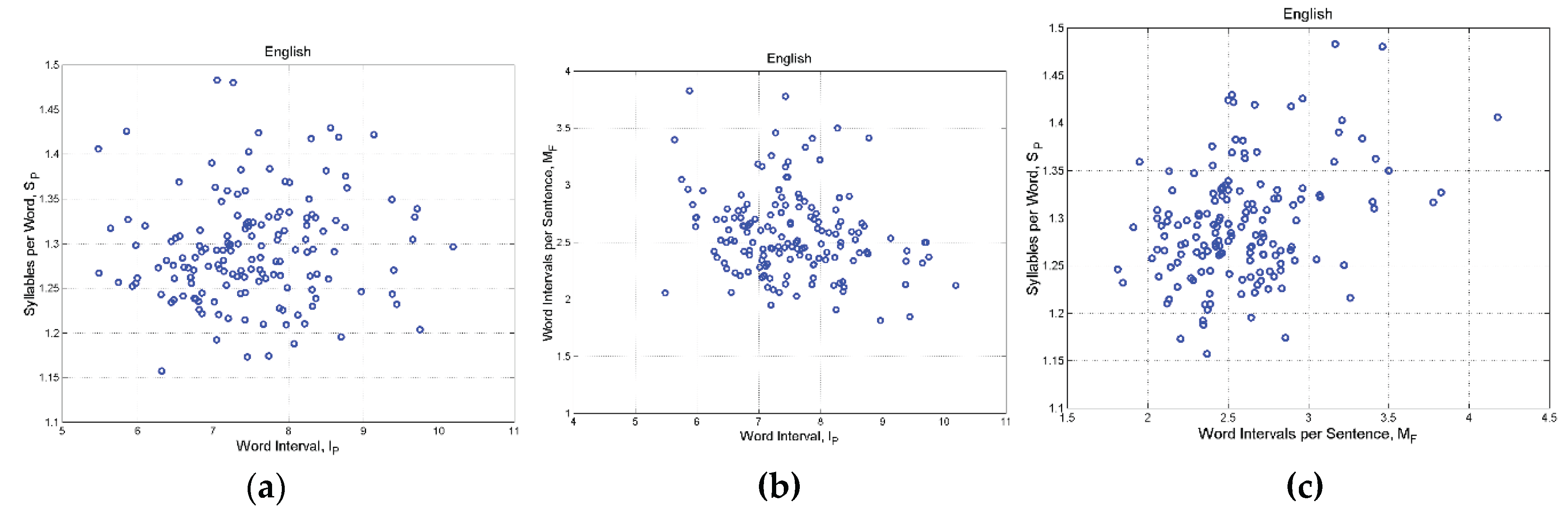
Figure 7.
Greek: (a) Scatterplot between and , the correlation coefficients between the logarithms of the variables is (b) Scatterplot between and , ; (c) Scatterplot between and , .
Figure 7.
Greek: (a) Scatterplot between and , the correlation coefficients between the logarithms of the variables is (b) Scatterplot between and , ; (c) Scatterplot between and , .
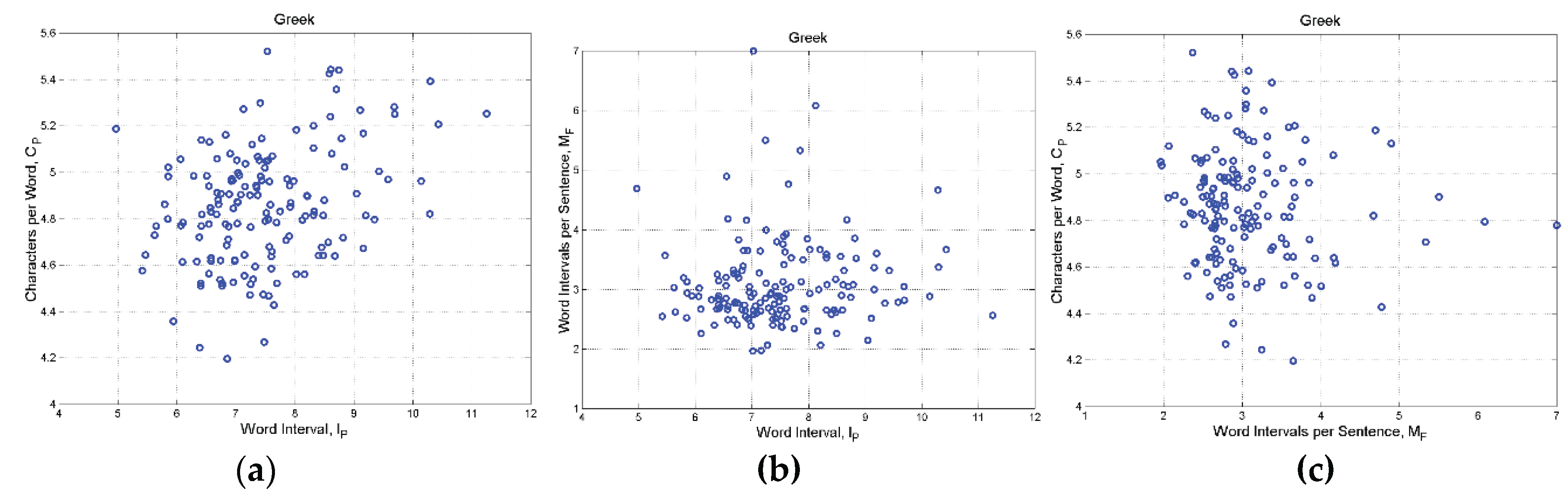
Figure 8.
(a) Log–normal probability density function of ; (b) Log–normal probability density function of
Figure 8.
(a) Log–normal probability density function of ; (b) Log–normal probability density function of
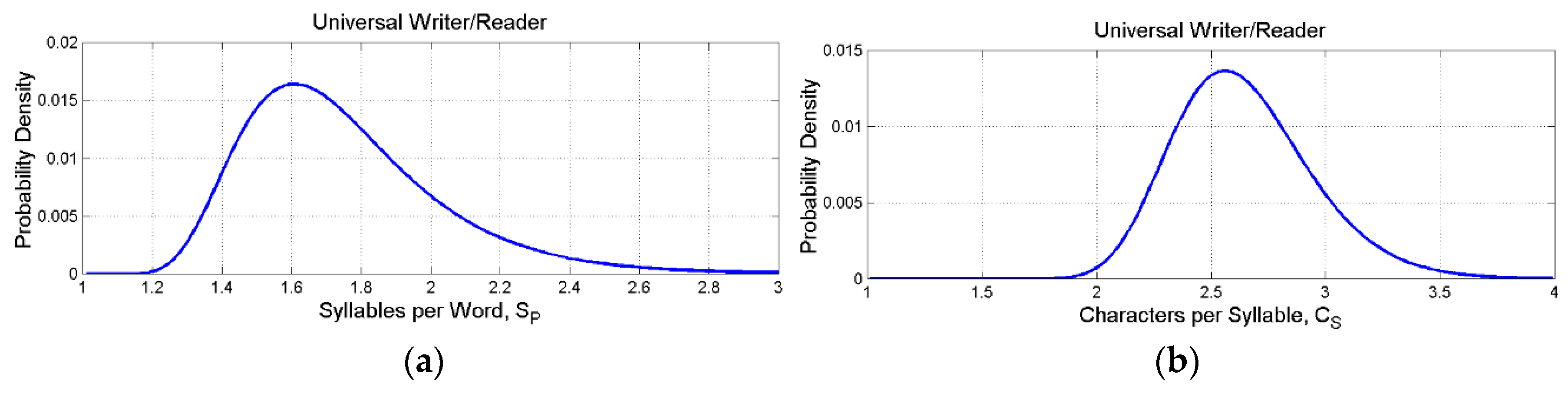
Figure 9.
(a) Log–normal probability density function of ; (b) Log–normal probability density function of .
Figure 9.
(a) Log–normal probability density function of ; (b) Log–normal probability density function of .
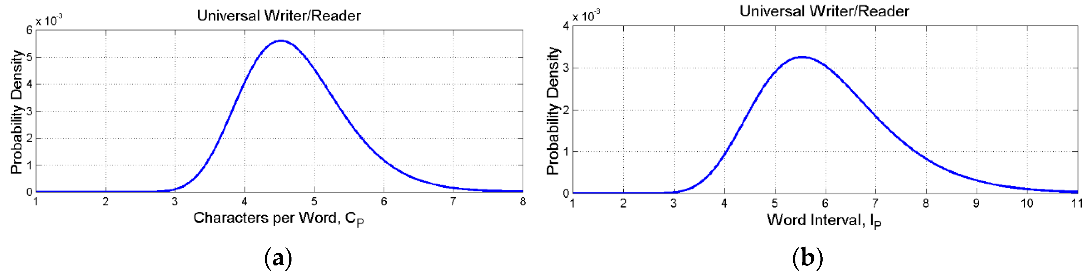
Figure 10.
(a) Log–normal probability density function of ; (b) Log–normal probability density function of .
Figure 10.
(a) Log–normal probability density function of ; (b) Log–normal probability density function of .
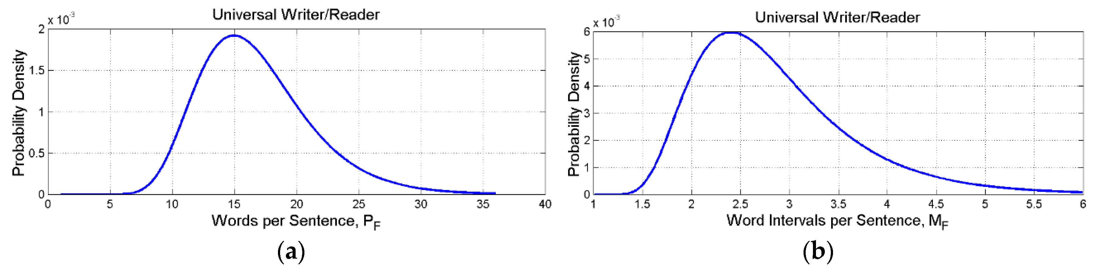
Figure 11.
Experimental (blue line, Monte Carlo simulations) probability density function of and its Gaussian model (black line).
Figure 11.
Experimental (blue line, Monte Carlo simulations) probability density function of and its Gaussian model (black line).
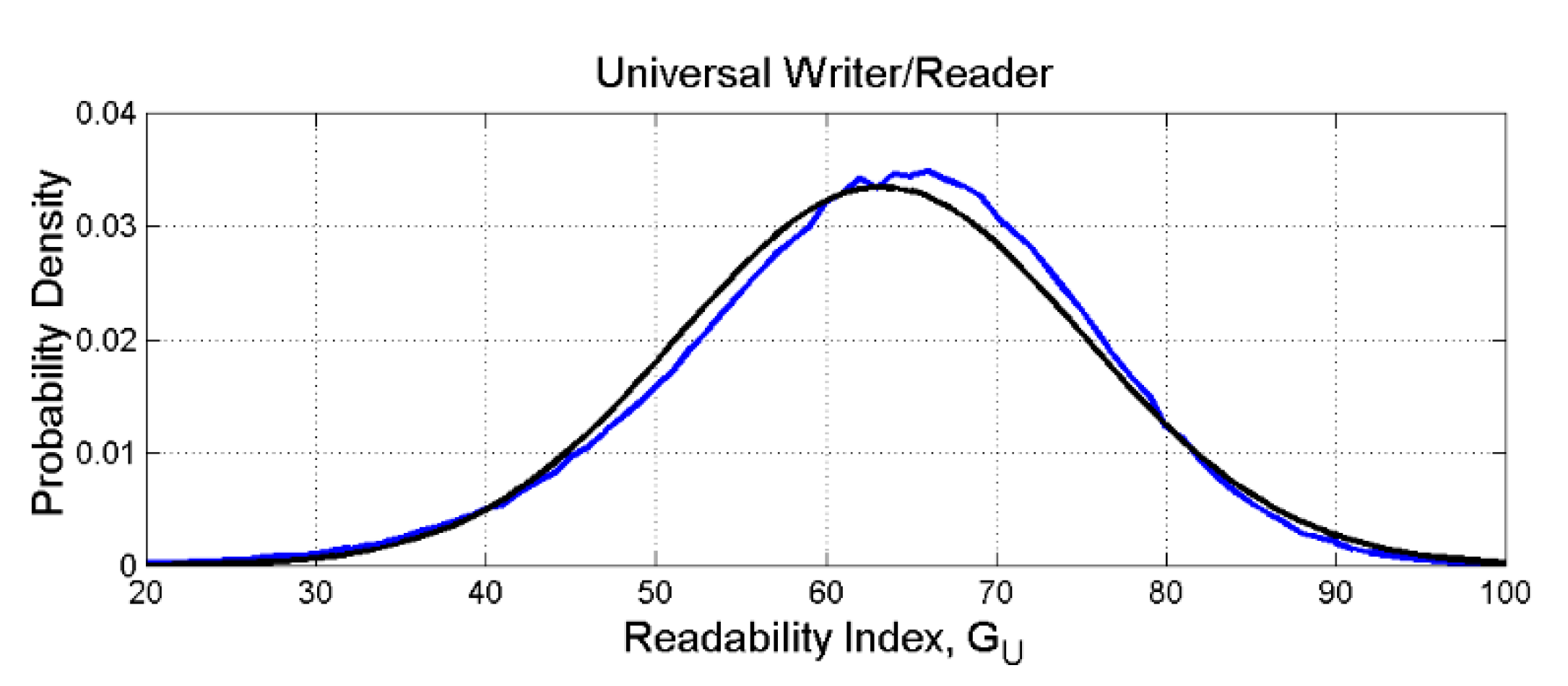
Figure 12.
Chart to estimate the number of school–years for a given , according to text reading difficulty (redrawn from Ref. [100]).According to Figure 12, texts with (universal mean value) would be “easy” to read by readers of about 8 school–years. The texts at standard deviation, namely and , would require, respectively, about 10 and 5.5 school–years.
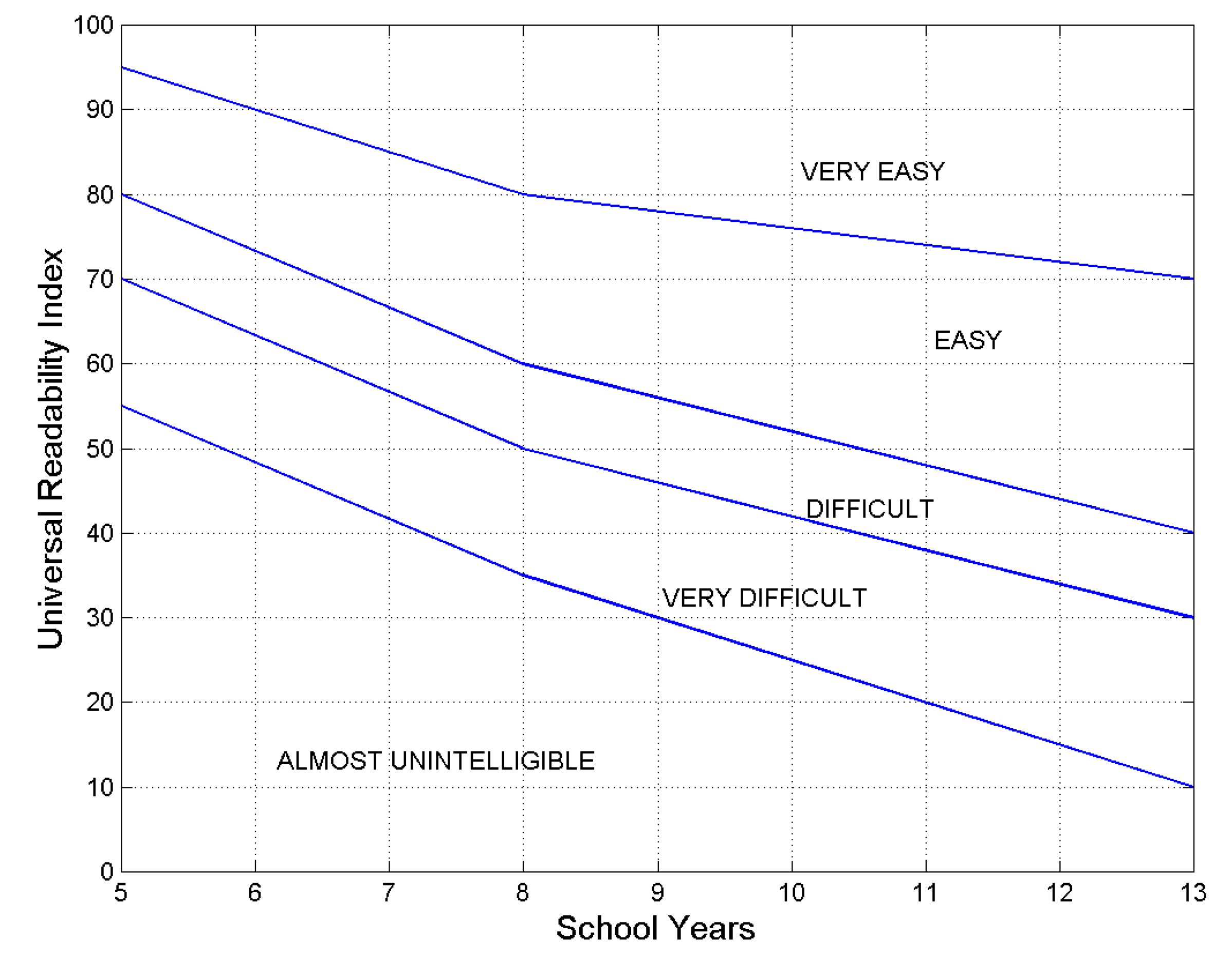
Figure 13.
Probability (%) that the readability index is greater than a certain value, versus number of school–years. Notice that in the ordinate scale decreases (reading difficulty increases) as increases. Examples of application: The horizontal red line – set, in this example, at 50% probability (i.e., it corresponds to ) – can cross texts declared “very difficult”, “difficult”, “easy” as the number of school years increase, therefore indicating that 50% of the texts are differently readable by readers of diverse schooling. The other red lines indicate standard deviation of . The magenta line set, in this example, at 8 school–years, shows that can cross percentages of texts declared “very easy”, “easy”, “difficult”, “very difficult”, “almost unintelligible”, therefore indicating percentages of texts with diverse reading difficulty.
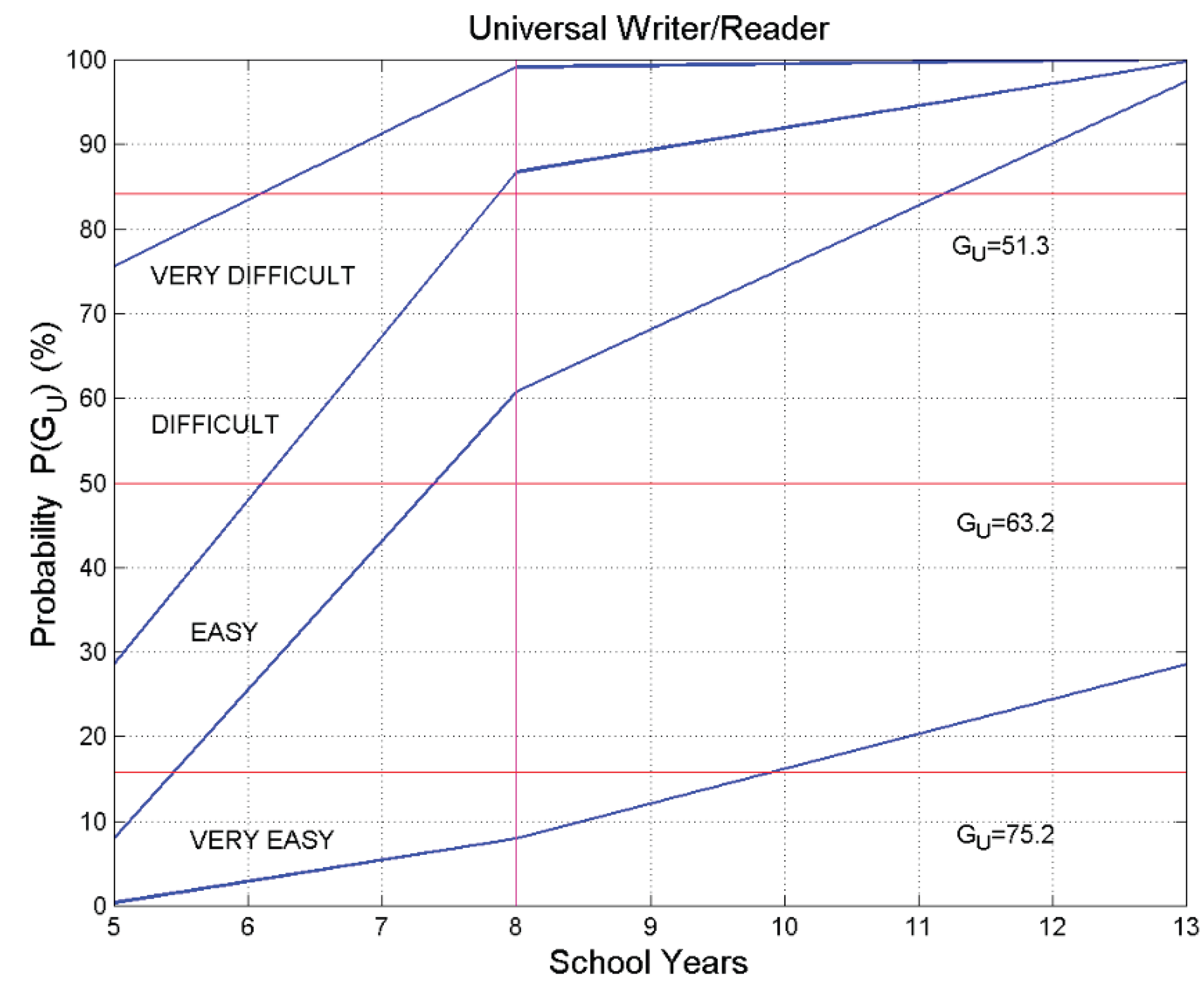
Table 1.
Mean value (left number of column, indicated by ) and standard deviation (right number, indicated by ) of the the surface deep−language parameters in the indicated language of the New Testament books (Matthew, Mark, Luke, John, Acts, Epistle to the Romans, Apocalypse,), calculated from 155 samples in each language. For example, in Greek with standard deviation . The list concerning the genealogy of Jesus of Nazareth reported in Matthew 1.1−1.17 17 and in Luke 3.23−3.38 was deleted for not biasing the statistics of linguistic variables. The source of the digital texts considered is reported in [78]. Languages with “*”: the statistics of and were calculated for the total number of samples (155 chapters per language); Languages with “°” the statistics of and were calculated only for Matthew (28 chapters per language).
| Language | Language Family | ||||||
|---|---|---|---|---|---|---|---|
| Greek | Hellenic | 23.07 6.65 | 7.47 1.09 | 4.86 0.25 | 3.08 0.73 | –– | –– |
| Latin | Italic | 18.28 4.77 | 5.07 0.68 | 5.16 0.28 | 3.60 0.77 | –– | –– |
| Esperanto | Constructed | 21.83 5.22 | 5.05 0.57 | 4.43 0.20 | 4.30 0.76 | –– | –– |
| French* | Romance | 18.73 2.51 | 7.54 0.85 | 4.20 0.16 | 2.50 0.32 | 1.47 0.05 | 2.85 0.05 |
| Italian* | Romance | 18.33 3.27 | 6.38 0.95 | 4.48 0.19 | 2.89 0.40 | 1.90 0.09 | 2.35 0.04 |
| Portuguese* | Romance | 16.18 3.25 | 5.54 0.59 | 4.43 0.20 | 2.93 0.56 | 1.85 0.09 | 2.40 0.05 |
| Romanian° | Romance | 18.00 4.19 | 6.49 0.74 | 4.34 0.19 | 2.78 0.65 | 1.82 0.05 | 2.35 0.04 |
| Spanish | Romance | 19.07 3.79 | 6.55 0.82 | 4.30 0.19 | 2.91 0.47 | 1.90 0.16 | 2.27 0.16 |
| Danish° | Germanic | 15.38 2.15 | 5.97 0.64 | 4.14 0.16 | 2.59 0.33 | 1.43 0.04 | 2.89 0.03 |
| English* | Germanic | 19.32 3.20 | 7.51 0.93 | 4.24 0.17 | 2.58 0.39 | 1.29 0.06 | 3.29 0.12 |
| Finnish° | Germanic | 17.44 4.09 | 4.94 0.56 | 5.90 0.31 | 3.54 0.75 | 2.27 0.05 | 2.57 0.03 |
| German* | Germanic | 17.23 2.77 | 5.89 0.60 | 4.68 0.19 | 2.94 0.45 | 1.51 0.07 | 3.10 0.07 |
| Icelandic | Germanic | 15.72 2.58 | 5.69 0.67 | 4.34 0.18 | 2.77 0.39 | –– | –– |
| Norwegian° | Germanic | 15.21 1.43 | 7.75 0.84 | 4.08 0.13 | 1.98 0.22 | 1.41 0.03 | 2.89 0.04 |
| Swedish° | Germanic | 15.95 2.17 | 8.06 1.35 | 4.23 0.18 | 2.01 0.31 | 1.50 0.04 | 2.80 0.05 |
| Bulgarian | Balto−Slavic | 14.97 2.61 | 5.64 0.64 | 4.41 0.19 | 2.67 0.43 | –– | –– |
| Czech° | Balto−Slavic | 13.20 3.10 | 4.89 0.65 | 4.51 0.21 | 2.71 0.61 | 1.80 0.05 | 1.80 0.05 |
| Croatian° | Balto−Slavic | 15.32 3.54 | 5.62 0.75 | 4.39 0.22 | 2.72 0.49 | 1.87 0.06 | 2.34 0.04 |
| Polish° | Balto−Slavic | 12.34 1.93 | 4.65 0.43 | 5.10 0.22 | 2.67 0.40 | 1.95 0.06 | 2.60 0.05 |
| Russian | Balto−Slavic | 17.90 4.46 | 4.28 0.46 | 4.67 0.27 | 4.18 0.92 | –– | –– |
| Serbian | Balto−Slavic | 14.46 2.42 | 5.81 0.69 | 4.24 0.20 | 2.50 0.39 | –– | –– |
| Slovak | Balto−Slavic | 12.95 2.10 | 5.18 0.61 | 4.65 0.23 | 2.51 0.36 | –– | –– |
| Ukrainian | Balto−Slavic | 13.81 2.18 | 4.72 0.41 | 4.56 0.26 | 2.95 0.58 | –– | –– |
| Estonian° | Uralic | 17.09 3.89 | 5.45 0.66 | 4.89 0.24 | 3.14 0.64 | 1.86 0.05 | 2.61 0.03 |
| Hungarian° | Uralic | 17.37 4.54 | 4.25 0.45 | 5.31 0.29 | 4.09 0.93 | 2.15 0.07 | 2.47 0.03 |
| Albanian | Albanian | 22.72 4.86 | 6.52 0.78 | 4.07 0.22 | 3.48 0.61 | –– | –– |
| Armenian | Armenian | 16.09 3.07 | 5.63 0.52 | 4.75 0.40 | 2.86 0.47 | –– | –– |
| Welsh | Celtic | 24.27 4.75 | 5.84 0.44 | 4.04 0.15 | 4.16 0.76 | –– | –– |
| Basque | Isolate | 18.09 4.31 | 4.99 0.52 | 6.22 0.27 | 3.63 0.81 | –– | –– |
| Hebrew | Semitic | 12.17 2.04 | 5.65 0.59 | 4.22 0.17 | 2.16 0.33 | –– | –– |
| Cebuano | Austronesian | 16.15 1.71 | 8.82 1.01 | 4.65 0.10 | 1.85 0.22 | –– | –– |
| Tagalog | Austronesian | 16.98 3.24 | 7.92 0.82 | 4.83 0.17 | 2.16 0.44 | –– | –– |
| Chichewa | Niger−Congo | 12.89 1.79 | 6.18 0.87 | 6.08 0.18 | 2.10 0.25 | –– | –– |
| Luganda | Niger−Congo | 13.65 2.78 | 5.74 0.82 | 6.23 0.23 | 2.39 0.40 | –– | –– |
| Somali | Afro−Asiatic | 19.57 5.50 | 6.37 1.01 | 5.32 0.16 | 3.06 0.65 | –– | –– |
| Haitian | French Creole | 14.87 1.83 | 6.55 0.71 | 3.37 0.10 | 2.28 0.26 | –– | –– |
| Nahuatl | Uto−Aztecan | 13.36 1.70 | 6.47 0.91 | 6.71 0.24 | 2.08 0.24 | –– | –– |
Table 2.
Comparison between mean values of and for Matthew (28 samples per language) and the NT data bank (155 samples per language) in the indicated languages. The standard deviation is reported in parentheses.
Table 2.
Comparison between mean values of and for Matthew (28 samples per language) and the NT data bank (155 samples per language) in the indicated languages. The standard deviation is reported in parentheses.
| Language | ||||||
|---|---|---|---|---|---|---|
| Matthew | NT | Matthew | NT | |||
| French | 1.46 (0.04) | 1.47 (0.05) | 2.86 (0.05) | 2.85 (0.05) | ||
| Italian | 1.89 (0.05) | 1.90 (0.08) | 2.27 (0.04) | 2.35 (0.04) | ||
| Portuguese | 1.84 (0.07) | 1.85 (0.08) | 2.42 (0.04) | 2.40 (0.05) | ||
| English | 1.27 (0.04) | 1.29 (0.06) | 3.29 (0.06) | 3.29 (0.11) | ||
| German | 1.50 (0.04) | 1.51 (0.07) | 3.10 (0.06) | 3.10 (0.07) | ||
Table 3.
Slope and correlation coefficient of the linear relationship , for the indicated language. The correlation coefficients are reported with four digits because they are all similar.
Table 3.
Slope and correlation coefficient of the linear relationship , for the indicated language. The correlation coefficients are reported with four digits because they are all similar.
| Language | Syllables versus Words | Characters versus Syllables | ||||
|---|---|---|---|---|---|---|
| Slope | Correlation coefficient | Slope | Correlation coefficient | |||
| French | 1.470 | 0.9949 | 2.849 | 0.9990 | ||
| Italian | 1.905 | 0.9912 | 2.347 | 0.9990 | ||
| Portuguese | 1.850 | 0.9909 | 2.401 | 0.9987 | ||
| English | 1.289 | 0.9930 | 3.275 | 0.9968 | ||
| German | 1.509 | 0.9914 | 3.087 | 0.9984 | ||
Table 4.
Fundamental statistics of the deep–language parameters.
| Deep–language parameter | ||||||
|---|---|---|---|---|---|---|
| –0.358 | 0.373 | 1.61 | 1.70 | 1.75 | 0.29 | |
| 0.479 | 0.184 | 2.56 | 2.62 | 2.64 | 0.31 | |
| 1.297 | 0.199 | 4.62 | 4.66 | 4.73 | 0.75 | |
| 1.581 | 0.261 | 5.79 | 5.86 | 6.03 | 1.33 | |
| 2.716 | 0.286 | 16.04 | 16.12 | 16.76 | 4.60 | |
| 0.526 | 0.434 | 2.50 | 2.69 | 2.86 | 0.85 |
Table 5.
Probability ranges corresponding to , , standard deviations of the log–normal model (Table 4), for the indicated deep–language parameters.
Table 5.
Probability ranges corresponding to , , standard deviations of the log–normal model (Table 4), for the indicated deep–language parameters.
| Probability range (%) | ||||||
|---|---|---|---|---|---|---|
Disclaimer/Publisher’s Note: The statements, opinions and data contained in all publications are solely those of the individual author(s) and contributor(s) and not of MDPI and/or the editor(s). MDPI and/or the editor(s) disclaim responsibility for any injury to people or property resulting from any ideas, methods, instructions or products referred to in the content. |
© 2025 by the authors. Licensee MDPI, Basel, Switzerland. This article is an open access article distributed under the terms and conditions of the Creative Commons Attribution (CC BY) license (http://creativecommons.org/licenses/by/4.0/).
Copyright: This open access article is published under a Creative Commons CC BY 4.0 license, which permit the free download, distribution, and reuse, provided that the author and preprint are cited in any reuse.


