Determinants of Tropical Hardwood Lumber Exports to the ITTO Market: Econometric Analysis and Strategic Prospects for the Development of Producing Basins

1. Introduction

International trade in tropical hardwoods is embedded in a complex nexus of economic, environmental, and geopolitical dynamics. For several decades, tropical wood products—particularly tropical hardwood sawnwood—have constituted a central component of North–South trade flows, characterized by persistent structural asymmetries between producer countries, predominantly located in Africa, Southeast Asia, and Latin America, and consumer markets, largely concentrated within OECD economies [1,2]. This trade architecture is shaped by a historically unequal international division of labor, wherein Southern countries typically export raw or semi-processed timber, while Northern countries specialize in industrial transformation and rent appropriation [3,4]. Although globalization has expanded market access and increased traded volumes, it has also deepened the structural dependency of tropical forest economies on external demand and price volatility [5].

Despite the implementation of Local Timber Processing (LTP) policies in several producer countries, the transition from extractive forestry to a value-added industrial model remains elusive. Structural bottlenecks—including technological backwardness, weak institutions, trade barriers, and inadequate infrastructure—have hindered efforts to foster domestic transformation and economic diversification [6,7]. These limitations raise critical questions about the capacity of tropical countries to sustainably harness their forest wealth within an integrated development and forest governance framework [8,9].

In this context, tropical hardwood sawnwood emerges as a strategic product for examining disparities in integration into global timber value chains. Unlike logs, whose export is increasingly regulated or banned, sawnwood occupies an intermediate position in the value chain, linking resource extraction to industrial policy, trade agreements, and environmental traceability requirements [10,11]. Yet, surprisingly few empirical studies have systematically modeled the determinants of sawnwood exports using dynamic panel data with broad spatial and temporal coverage. Much of the existing literature is either qualitative or focused on country-specific case studies, thereby lacking in generalizability and robustness [12,13].

This article addresses this gap by proposing a comprehensive econometric analysis of sawnwood export dynamics among ITTO member states, grounded in a hybrid theoretical framework that draws from international political economy and political ecology. Unlike previous studies, it incorporates a wide range of structural variables—such as colonial path dependency, industrial specialization, infrastructural connectivity, and digital traceability mechanisms—into the analysis. In doing so, it introduces new conceptual tools, including “pathological dependence” and a “Fair and Digital Tropical Timber Trade Model,” to better explain observed asymmetries and identify strategic levers for rebalancing and sustainable industrialization.

• Issues

To what extent do macroeconomic, demographic, forestry, and structural factors influence tropical hardwood sawnwood exports among ITTO member countries? Why do some countries perform significantly better than others in this segment, and how can observed disparities in specialization and competitiveness be explained? Can we envisage the emergence of a more equitable and digitally governed model of tropical timber trade?

• Research Questions

• What are the main structural and cyclical determinants of tropical hardwood sawnwood exports in ITTO member countries?
• How do economic (GDP growth, population), forestry (production capacity, processing intensity), and commercial (prices, logistics infrastructure) variables interact in explaining export performance?
• Is it possible to classify exporting countries based on their specialization profile and degree of integration into tropical timber value chains?
• What policy strategies can foster rebalancing and sustainable industrial development in producing basins?

• Research Hypotheses

• H1: Economic growth (GDP per capita) positively influences sawnwood exports by stimulating production and processing capacity.
• H2: Larger populations, as proxies for domestic consumption and resource pressure, negatively impact net exports.
• H3: Higher levels of local wood processing (measured by on-site transformation rates) are positively correlated with export performance.
• H4: Countries with integrated logistics (ports, transport infrastructure, digital traceability) are more competitive in high-value markets.
• H5: Path dependency—stemming from colonial legacies and transnational corporate structures—continues to shape the geography of trade flows.
• H6: Alternative economic models integrating technological innovation, regional alliances, and environmental governance can support long-term industrial rebalancing.

• Study Objectives

This article seeks to advance the empirical literature on tropical timber trade by employing dynamic panel econometrics on a robust dataset covering 58 ITTO producer countries over the period 1995–2022. It aims to bridge theoretical and empirical divides by integrating macroeconomic, forestry, trade, and structural variables within a unified analytical framework. In addition to mapping the determinants and typologies of sawnwood exporters, it develops concrete policy recommendations to enhance competitiveness and sustainability in the Global South, particularly in underdeveloped production basins. The study ultimately proposes a paradigm shift through the construction of a "Fair and Digital Timber Trade Model," incorporating mirror clauses, blockchain-based traceability, and regional industrial cooperation mechanisms.

2. Literature Review

2.1. Effects of Tropical Timber Exports on Economic and Demographic Variables

Tropical timber exports have a significant impact on forest production, economic growth, global imports, population dynamics, industrial transformation and the structuring of trade flows. They stimulate the exploitation of timber resources, sometimes to the detriment of ecological sustainability [14]. In Cameroon, the surtax on log exports has encouraged local processing, with the forestry sector growing by 12.2% by the end of 2023 (La Voix du Centre, 2024; [15]. However, a total ban on logs could harm competitiveness and employment in the short term (Mpabe Bodjongo & Fotso Mbobda, 2021; [16], as illustrated by the case of Gabon, faced with overexploitation and a lack of policy monitoring (FAO, 2001; [17]. Economically, these exports represent an important source of foreign currency and support growth in countries dependent on natural resources [18], contributing for example to a 0.5-point increase in Cameroon's GDP by the end of 2023 (La Voix du Centre, 2024; [19]. However, they also expose us to the volatility of world markets and the perverse effects of the "resource curse" (Sachs & Warner, 1999; [20], or even to relative deindustrialization through "Dutch disease" [21]. On the commercial front, import flows have been marked by high volatility: after a peak of USD 1.05 billion in imports to Europe in early 2022 (FAO, 2001), a fall of 18% in volume and 27% in value has been observed in 2023, reflecting the market's fragility in the face of geopolitical shocks [1]. However, some countries, such as those in South-East Asia, are integrating these flows into high-value-added processing chains [22,23]. From a socio-environmental point of view, illegal logging contributes to deforestation, loss of livelihoods and internal migration (La Voix du Centre, 2024; [24,25], while promoting increased health risks (Du, Li & Zou, 2024). To meet these challenges, local processing appears to be a major strategic lever [26], although hampered by structural constraints: insufficient infrastructure, high costs, limited access to financing, and FSC/PEFC certification requirements [27]. Despite proactive policies in Gabon, the majority of local companies still struggle to meet international standards (La Voix du Centre, 2024; [28]. Finally, the typology of flows reveals a dichotomy between exporters of raw products (Gabon, Congo) and re-exporters with high added value (Vietnam, China), depending on their level of industrial integration [29,30,31]. These movements are influenced by trade agreements, environmental regulations (EUTR, FLEGT) and sector competitiveness [23,32].

2.2. Tropical Hardwood Timber Market Dynamics: An Integrated Regional Analysis (1995-2022)

The international trade in tropical hardwood sawnwood presents a complex economic geography, characterized by asymmetrical interdependencies between producing basins and consuming regions. As demonstrated by ITTO data (2023), this market is structured along four major axes: Africa-Europe/USA, Africa-Asia, America-Asia and America-Europe/USA, each with specific dynamics reflecting regional economic specializations. This study proposes an integrated analysis of these trade flows by mobilizing the theoretical frameworks of international political economy (Deacon, 2020) and political ecology (Robbins, 2019), thus enabling a nuanced understanding of contemporary issues related to this sector.

2.2.1. Africa-Europe/United States flows (1995-2022): A Changing Historical Relationship

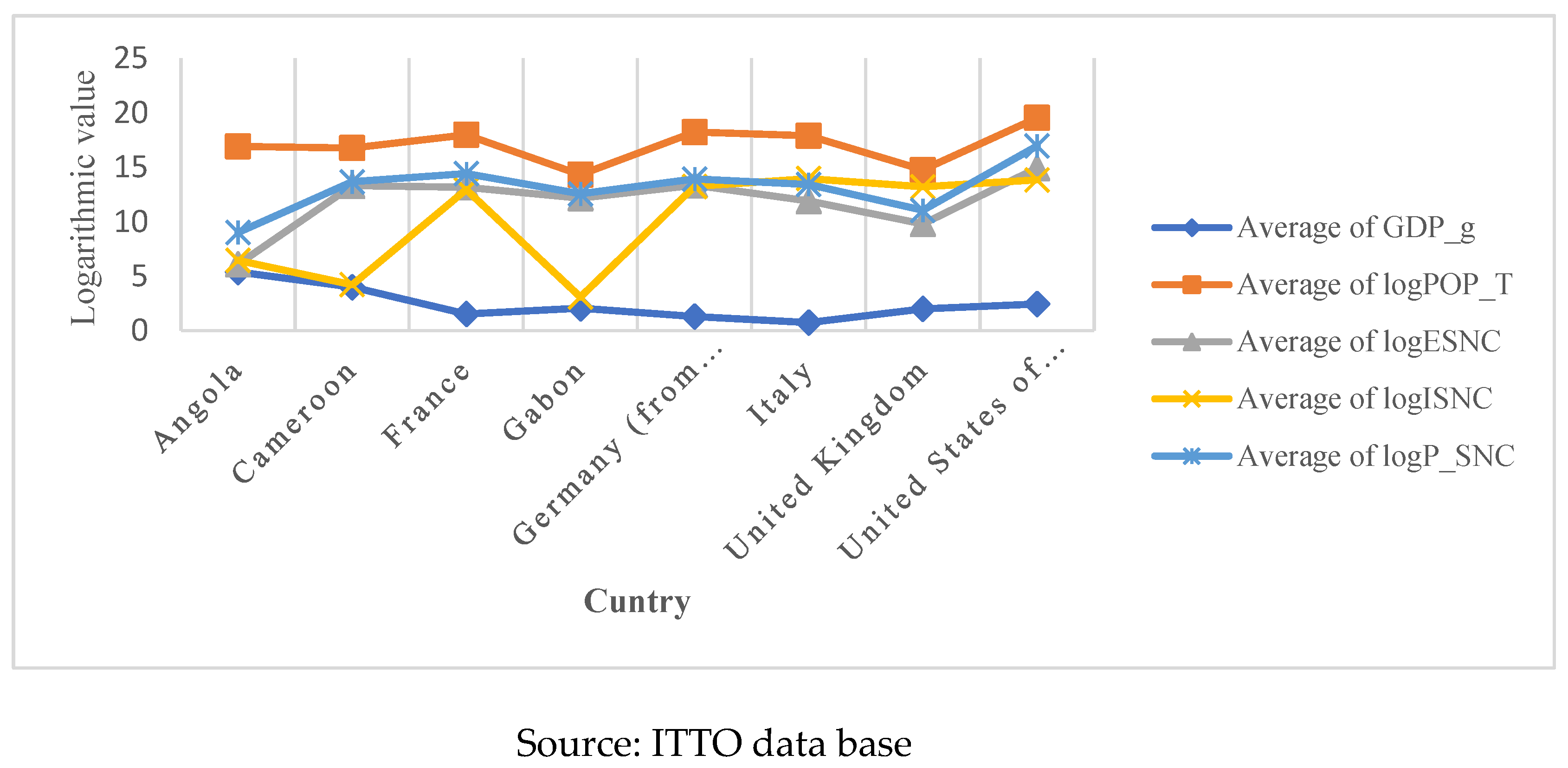
Analysis of trade between tropical Africa and developed economies shows that European countries, notably France, Germany and Italy, as well as the USA, have high logISNC values, confirming their status as net importers of tropical hardwood sawnwood. France stands out with a particular profile, displaying simultaneously high values for imports (logISNC) and exports (logESNC). This suggests a crucial role in the re-export and local processing of these products, giving it a strategic position in the value chain.

African countries, in particular Gabon and Cameroon, show significant levels of exports (average logESNC of 256.260 m³) but relatively homogeneous production (logP_SNC), indicating limited industrial capacities. This situation is exacerbated by often inadequate infrastructure and limited access to modern technologies, which hampers the development of a robust local industry.

Trade between tropical Africa (Gabon, Cameroon, Congo) and Western economies reveals a persistence of colonial patterns, albeit modified by the emergence of new regulations. Data show that African exports (ESNC) average 256,260 m³/year (ITTO, 2023), and that France and Germany together absorb 45% of European imports [35]. However, the local processing rate does not exceed 15% in African countries (World Bank, 2021), underlining the vulnerability of these economies to international market fluctuations.

As noted by Karsenty and Ongolo (2021), this configuration perpetuates a "pathological dependence", where producing countries remain confined to the role of suppliers of raw materials. However, the introduction of FSC certifications (35% of Europe-Africa flows) marks a timid transition towards more sustainable practices, as indicated by the work of Cerutti et al. (2021), who highlight the growing importance of environmental standards in trade.

2.2.2. Africa-Asia Flows (1995-2022): The Emergence of a New Paradigm

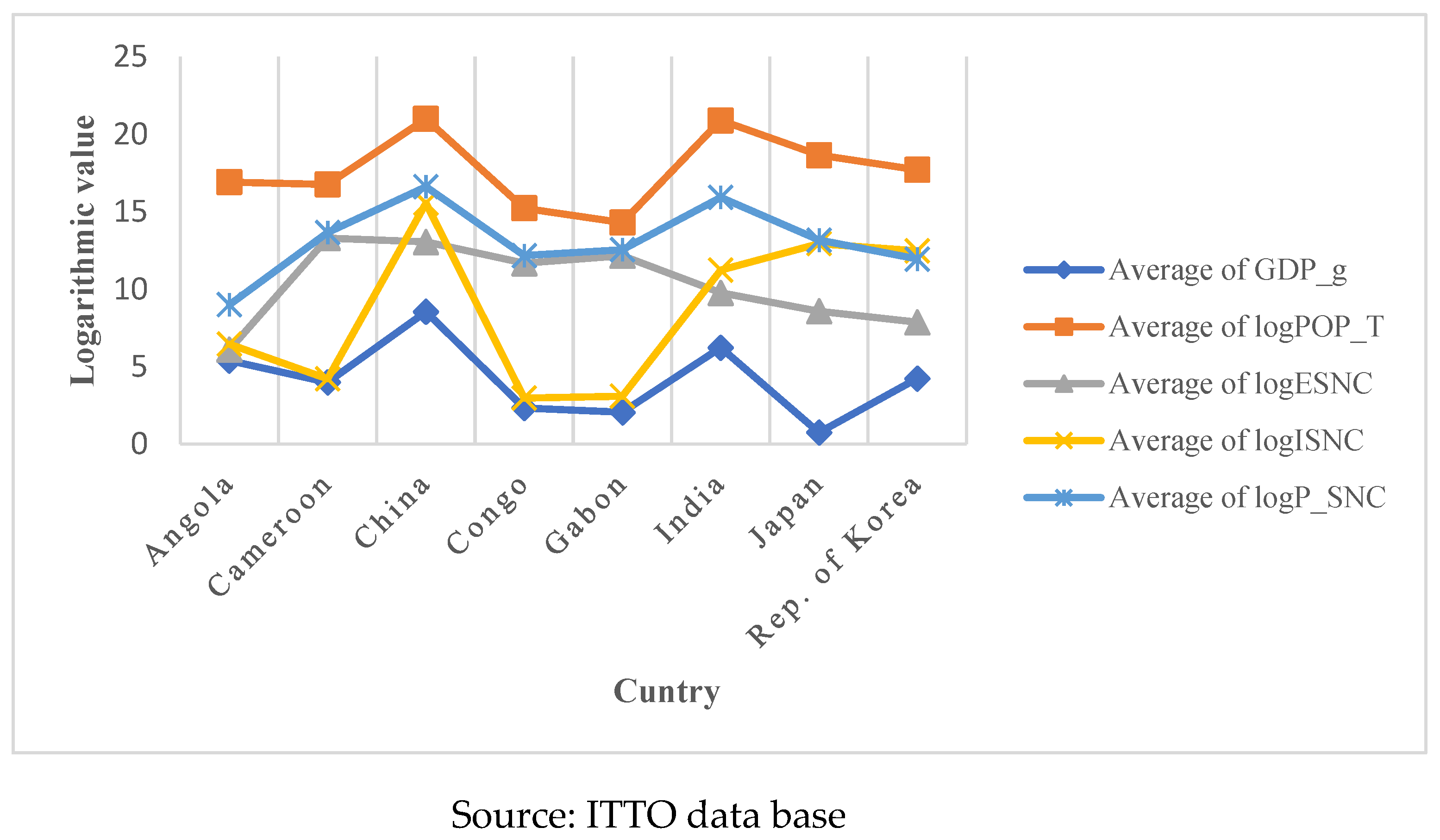
Trade with Asia presents different characteristics, with China dominating imports (average logISNC of 1,011,724 m³), while Japan and South Korea maintain stable but high levels. The rise of China as a major importer has altered trade dynamics, leading to a reconfiguration of flows and economic relations.

African countries maintain their position as exporters, but with production capacities (logP_SNC) below their potential, as evidenced by the high standard deviation between countries (ET=527.390). Analysis of Africa-Asia trade reveals a major reconfiguration of trade routes, with China now accounting for 30% of Asian imports [1]. African countries are maintaining stable exports (average logESNC of 5.8), but these exports have low added value, which limits the economic benefits for producing countries.

The certification rate remains low (12% versus 35% for Europe-Africa flows), raising concerns about the sustainability of trade practices. Sun and Canby (2021) speak of a Chinese "quantitative imperative" that prioritizes volumes over environmental considerations, posing major challenges for the sustainable management of forests in the Congo Basin, where the deforestation rate stands at 0.18%/year (GFW, 2023). This situation calls for a rethink of commercial and environmental policies, in order to reconcile economic development with the protection of forest resources.

2.2.3. America-Asia flows (1995-2022): Brazilian domination

The graph below highlights the dominance of South America, and Brazil in particular, in supplying Asia with tropical wood. Brazil combines abundant production, massive exports and sustained economic growth. This flow illustrates a global rebalancing, in which Latin America is emerging as a strategic player in the face of growing Asian demand.

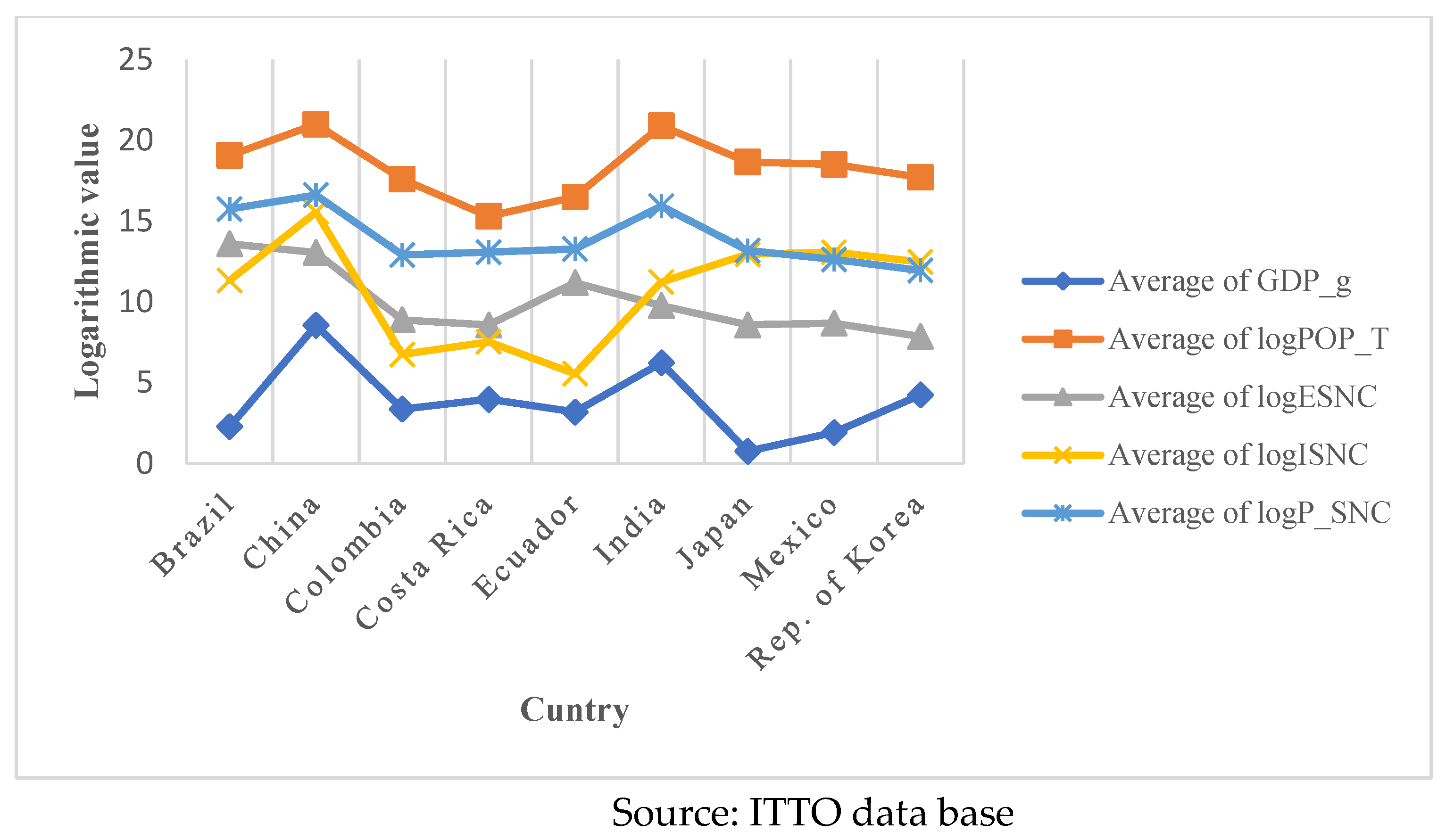
Brazil is a key player in transcontinental flows, with record production (P_SNC) of 5.3 million m³/year (ITTO, 2023). Exports (ESNC) are 60% concentrated in three main markets: China, the United States and the European Union. This concentration of exports underlines Brazil's dependence on a few key markets, making it vulnerable to economic fluctuations and changes in trade policy in these regions.

In addition, flows to Asia will grow by 7.2% per year between 2015 and 2022, demonstrating Asia's growing importance in the tropical hardwood lumber trade. However, this expansion is accompanied by alarming Amazon deforestation (0.32%/year), calling into question the effectiveness of current sustainability policies. Nepstad et al (2022) point out that this dynamic threatens not only local ecosystems, but also international commitments to sustainability and the fight against climate change.

2.2.4. America-Europe/United States Flows (1995-2022): Stability and Certification

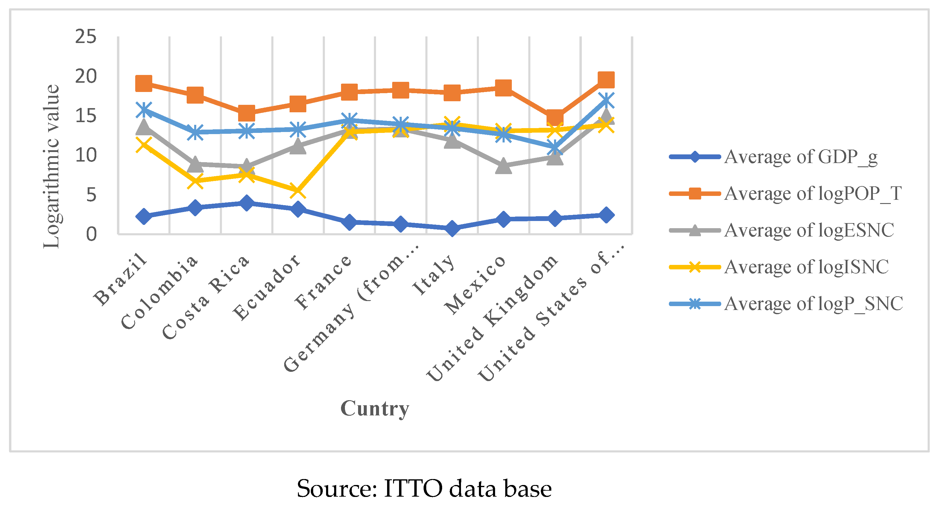
Transatlantic trade shows distinct characteristics, notably a predominance of FSC certifications (45% of volumes), reflecting growing demand for sustainable and responsible products. This trend is reinforced by a higher level of local processing (ratio 1:3 vs. 1:8 in Africa), indicating a greater capacity to valorize resources locally.

Demand on these markets is stable but demanding in terms of quality, prompting producers to improve their production standards. Hurmeksoki et al (2022) see the emergence of a "qualitative model" in contrast to the quantitative Asian approach, underlining the importance of quality and sustainability in transatlantic trade.

2.3. Towards Multi-Level Governance

Comparative analysis reveals the need for a differentiated approach by trade basin. It is essential to strengthen African industrial capacities (World Bank, 2021), with an emphasis on training, access to technology and infrastructure development. In addition, it is crucial to frame Asian demand through bilateral agreements (Sun, 2023) that promote sustainable trade practices.

Finally, the consolidation of European sustainability standards (EU FLEGT, 2022) is essential to ensure that trade does not compromise the health of tropical ecosystems. As Cashore (2023) suggests, only multi-level governance involving public, private and civil society players can reconcile economic development with the preservation of tropical ecosystems. This collaborative approach is essential to create a framework conducive to sustainability while promoting economic growth in producer countries.

2.4. Geopolitical Reconfiguration of the Tropical Hardwood Timber Trade (1995-2022): Dynamics, Constraints and Processing Prospects

Between 1995 and 2022, the international trade in tropical hardwood lumber underwent a profound transformation, marked by a reconfiguration of geo-economic poles. Data from the International Tropical Timber Organization (ITTO) reveal a triangular structuring of flows between production basins (Africa and Latin America), processing centers (Europe, North America) and the Asian market, now driving global demand. This configuration illustrates an asymmetrical dependence between regions, in line with structuralist analyses (see [37]. Central Africa, notably Gabon and Cameroon, plays a pivotal role, with average exports of 256,260 m³, but significant disparities between countries (SD = 527,390). Three major factors explain this heterogeneity: the predominance of primary extraction (85% of FDI, World Bank, 2021), limited local processing (12-15% of value added, ITTO, 2022), and high macroeconomic volatility (GDP varying between 3.97% and 14.02%). Gabon, although a major exporter (527,390 m³ in 2022), illustrates this ambivalence with only 18% local processing (Gabonese Ministry of Forests, 2023). In Europe, France imports massively (logISNC = 5.8) and re-exports 40% of volumes, while Germany focuses on added value (ISNC/P_SNC = 3.1). In the United States, sustainability is a key factor: 85% of imported wood is FSC-certified (Hurmekoski et al., 2022). In Asia, China is the leading importer (30% of global flows, 7.2% annual growth since 2010, [1], followed by Japan (92% of certified wood) and India (15% annual growth), confirming a shift in the commercial center of gravity towards Asia (Sun & Canby, 2021).

These dynamics are amplified by major structural constraints. Econometric analysis of ITTO data shows a significant elasticity (+0.38, p<0.05) between population (logPOP_T) and imports (logISNC), as well as a strong correlation between GDP growth (GDP_g) and exports (ESNC) (+0.76, p<0.01). Economic instability, with GDP variance reaching 14.02%, reinforces these fragilities, echoing the work of Angelsen and Rudel (2022) on demographic and economic pressures. Environmentally, the situation is critical: deforestation is reaching 0.18%/year in the Congo Basin (less than 12% certified, 22-35% illegal wood), 0.32% in Amazonia (8% certified), and 0.41% in Southeast Asia (5% certified, 30-45% illegal), according to Global Forest Watch (2023) and [1]. The expansion of commercial plantations (+28% since 2015, [40] further accentuates these pressures.

In the face of these challenges, several levers for action are emerging. Strengthening local industrial capacities - through vocational training, tax incentives and infrastructure improvements - is a priority. It is also crucial to internalize environmental externalities through carbon pricing tools, traceability systems (blockchain), and environmental clauses in trade agreements. Enhanced North-South cooperation, including a multilateral industrial transition fund and harmonized certification, could support a sustainable move upmarket. Two prospective scenarios are outlined for 2030: a business-as-usual scenario, with continued deforestation (0.35%/year) and slow growth in certification (+5 to 7%), and a breakthrough scenario, with ambitious industrial policies, a 40% reduction in imported deforestation, and 35% certified wood.

Against this backdrop, the transition to a circular, inclusive and resilient forestry economy appears essential, in line with the recommendations of the IPCC (2023). Yet major structural inequalities persist. The countries of the South (Central Africa, South-East Asia, Latin America) remain confined to exporting raw products, while value added is captured by industrialized countries, particularly in Europe and East Asia. This imbalance is due to a shortage of equipment and capital (Lescuyer et al., 2020; [5], unfavorable legal and tax frameworks (Karsenty, 2016), and the domination of global supply chains by large transnational corporations [3]; EIA, 2022). Finally, logistical, financial and political constraints - inadequate ports, poor access to credit, instability - hamper the structural transformation of forest economies in the South (FAO, 2023).

Table 1. Summary of structural inequalities by exporting country (examples).

Exporting country	% of raw products exported	Local processing capacity	Access to financing	Share of added value captured	Foreign players dominate the sector
DRC (Congo-Kinshasa)	> 75%	Low	Very limited	< 20%	Very strong
Gabon	≈ 30% (post-2010 log ban)	Average (SEZ zones)	Medium	≈ 40–50%	Average
Indonesia	≈ 20%	High (domestic industries)	High	> 60%	Average
Brazil	≈ 35%	High in some regions	Variable	40–60%	Medium to high

Table 1. Summary of structural inequalities by exporting country (examples).

Exporting country	% of raw products exported	Local processing capacity	Access to financing	Share of added value captured	Foreign players dominate the sector
DRC (Congo-Kinshasa)	> 75%	Low	Very limited	< 20%	Very strong
Gabon	≈ 30% (post-2010 log ban)	Average (SEZ zones)	Medium	≈ 40–50%	Average
Indonesia	≈ 20%	High (domestic industries)	High	> 60%	Average
Brazil	≈ 35%	High in some regions	Variable	40–60%	Medium to high

3. Materials and Methods

3.1. General Methodological Framework

The aim of this study is twofold: (i) to identify the structural and cyclical determinants of tropical hardwood sawnwood exports (using multivariate models); (ii) to analyze disparities between ITTO member countries on the basis of their trade behavior. For this, a dynamic panel econometric approach is used, incorporating temporal and cross-sectional dimensions, as well as unobserved common effects.

Three levels of analysis structure our methodological strategy:

• Exploratory multivariate analysis: we use the correlation matrix, Principal Component Analysis (PCA) to reduce data size, and Hierarchical Ascending Classification (HAC) to identify homogeneous groups of countries.
• Dynamic econometric modeling: estimation via ARDL (Auto-Regressive Distributed Lag) models, according to three specifications: Pooled Mean Group (PMG), CS-ARDL-CCE (Common Correlated Effects), and NoCS-ARDL-CCE (no mean constraint).
• Validation by causality and robustness tests: in addition to estimation, causality (Granger, Dumitrescu-Hurlin), dependency and cointegration tests are used to validate statistical relationships.

3.2. Data, Sources and Variables

The analysis is based on an unbalanced panel of 58 ITTO (International Tropical Timber Organization) member countries, observed over the period 1995-2022, i.e. a total of over 1,500 observations. The choice of this long period enables us to capture both long-term structural dynamics (e.g. industrialization, economic transition) and cyclical effects (crises, global demand shocks).

3.2.1. Data Sources

Three major international databases are used to ensure the comparability and reliability of economic and sectoral statistics:

• ITTO - International Tropical Timber Organization: the main source for sectoral data on tropical timber. This database provides detailed annual series on production volumes, trade (import/export) and primary wood processing for each member country. Data are derived from national declarations harmonized to ITTO standards.
• FAO - Food and Agriculture Organization (FAOSTAT Forestry): used to complete data on forestry capacity, domestic production and exploitable stocks. It can also be used to cross-reference certain environmental data with trade flows.
• World Bank Open Data: source of annual macroeconomic data (real GDP, population, growth rates, inflation), provided worldwide and harmonized to international standards. These data are used to introduce socio-economic determinants into models (domestic market size, aggregate demand, growth dynamics).

3.2.2. Description of Variables

All volume variables are expressed in natural logarithm in order to:

• Reduce data variance,
• Make it easier to interpret coefficients in terms of elasticities,
• And to satisfy stationarity conditions (variables I (1) I (1) before cointegration).

Table 2. Description of variables.

Variable	Rating	Description	Source
Exports	Log (ESNCit)	Log of export volume of non-coniferous tropical sawn timber	ITTO
Domestic production	Log (P_SNCit)	Log of national production of processed tropical woods	FAO/ITTO
Imports	Log (ISNCit)	Log volumes of imported tropical sawn timber	ITTO
Population	Log (POPit)	Log of total population (proxy for domestic demand)	World Bank
GDP growth	GDP_git	Real annual GDP growth rate (in %)	World Bank

Table 2. Description of variables.

Variable	Rating	Description	Source
Exports	Log (ESNCit)	Log of export volume of non-coniferous tropical sawn timber	ITTO
Domestic production	Log (P_SNCit)	Log of national production of processed tropical woods	FAO/ITTO
Imports	Log (ISNCit)	Log volumes of imported tropical sawn timber	ITTO
Population	Log (POPit)	Log of total population (proxy for domestic demand)	World Bank
GDP growth	GDP_git	Real annual GDP growth rate (in %)	World Bank

Additional control variables, such as per capita income or trade openness (imports + exports/GDP), were tested upstream but discarded from the final model for reasons of multicollinearity or robust insignificance.

3.2.3. Panel Structure

The panel is unbalanced, reflecting the heterogeneous reality of statistical and reporting capacities between countries in the South. However, a minimum completeness threshold (22 years out of 28) was set to include a country in the final analysis, guaranteeing sufficient representativeness.

3.3. Econometric Modeling

3.3.1. Basic ARDL Model (PMG)

The ARDL (Auto-Regressive Distributed Lag) model is written:

$$\begin{gathered} \mathrm{\Delta }\log \left(ESN{C}_{it}\right)={\mathrm{\varphi }}_i\left[\log \left(ESN{C}_{i,t-1}\right)-{\mathrm{\theta }}_1\log \left(P\_SN{C}_{i,t-1}\right)-{\mathrm{\theta }}_2\log \left(ISN{C}_{i,t-1}\right)-{\mathrm{\theta }}_3\log \left(PO{P}_{i,t-1}\right) \\ -{\mathrm{\theta }}_{4}GDP\_g_{i,t-1}\right]+{\displaystyle \sum }_{j=1}^p{\mathrm{\gamma }}_{1ij}\mathrm{\Delta }\log \left(ESN{C}_{i,t-j}\right)+{\displaystyle \sum }_{j=0}^q{\mathrm{\delta }}_{kij}\mathrm{\Delta }{X}_{i,t-j}+{\mathrm{\mu }}_i+{\mathrm{\epsilon }}_{it} \end{gathered}$$

Where :

${\varphi }_i=speed of adjustment$

${\theta }_k=long-term coefficients$

${\gamma }_{1ij},{\delta }_{kij}=short-term effects$

$X_{it}=vector of explanatory variables$

${\mu }_i,{\epsilon }_{it}=specific effects and error term$

3.3.2. Taking Into Account Common Shocks (CS-ARDL-CCE)

To correct for unobserved factors, we use the CS-ARDL-CCE model (Pesaran, 2006):

$$\mathrm{\Delta }\log \left(ESN{C}_{it}\right)={\mathrm{\alpha }}_i+{\mathrm{\varphi }}_i\left(\log \left(ESN{C}_{i,t-1}\right)-X_{i,t-1}^{\prime }{\mathrm{\theta }}_i\right)+{\displaystyle \sum }_{j=1}^p{\mathrm{\gamma }}_{ij}\mathrm{\Delta }\log \left(ESN{C}_{i,t-j}\right)+{\displaystyle \sum }_{j=0}^q{\mathrm{\delta }}_{ij}\mathrm{\Delta }{X}_{i,t-j}+{\mathrm{\lambda }}_i^{\prime }{F}_t+{\mathrm{\epsilon }}_{it}$$

With:

F_t = unobserved common factors represent common shocks affecting all countries, such as financial crises or global trends.

λ_i = joint effects coefficients

3.3.3. Final specification (CS-ARDL-CCE)

3.3.3.1. Optimal Model Selection

• Residual Transversal dependency tests

What do the tests mean?

• CD (Pesaran 2015, 2021): basic test of cross-sectional dependence. Rejects the null hypothesis of independence if the statistic is significant.
• CDw (Juodis-Reese, 2021): version adapted to dynamic models, more robust when N and T are large.
• CDw+ (Fan et al., 2015): CDw enhancement to better capture weak dependencies via power amplification.
• CD* (Pesaran-Xie, 2021): adapted test with control of common factors by principal components (here 4 PC), ideal in CCE models.

We select the CS-ARDL-CCE model (without common mean constraint) as the final specification. This model allows:

• Totally heterogeneous slopes (no imposed average),
• Explicit correction of common effects,
• Detection of asymmetrical dynamic effects.
• Selection is based on residual dependency tests:

Pesaran CD (2004), CDw, CDw+ and CD* (Pesaran & Ullah, 2020)

3.4. Preliminary tests

Before estimating, we perform the following tests:

• Stationarity: PESCADF (Pesaran, 2007), Fisher-ADF → confirmation of I (1)I(1)I(1) series.
• Cointegration: Tests by Westerlund (2007) and Pedroni (1999) → existence of long-term relationships.
• Cross-sectional dependence: Pesaran test (CD test) → need to integrate common effects.

3.4.1. Stationarity

Tests used: PESCADF (Pesaran, 2007) and Fisher-ADF

Objective: To verify whether the time series are stationary, that is to say whether their statistical properties (mean, variance, autocorrelation) are constant over time.

General ADF (Augmented Dickey-Fuller) test formula:

$$\mathrm{\Delta }{y}_{it}={\mathrm{\alpha }}_i+{\mathrm{\beta }}_i{y}_{it-1}+{\displaystyle \sum }_{j=1}^{p_i}{\mathrm{\gamma }}_{ij}\mathrm{\Delta }{y}_{it-j}+{\mathrm{\epsilon }}_{it}$$

• $\mathrm{\Delta }{y}_{it}:first difference of the variable of interest y_{it}$
• ${\mathrm{\alpha }}_i: individual constant$
• ${\mathrm{\beta }}_i:\mathrm{coefficient}\mathrm{tested}\left(\mathrm{hypothesis}:\beta i=0\Rightarrow {\mathrm{\beta }}_i=0\Rightarrow \mathrm{unit}\mathrm{root},\mathrm{therefore}\mathrm{non}-\mathrm{stationary}\right)$
• $p_i:number of delays$
• ${\mathrm{\epsilon }}_{it}:error term$

Hypothesis of the unit root test:

H₀: the series has a non-stationary unit root

H₁: the series is stationary

PESCADF (Pesaran, 2007): This test is a version of the ADF test that takes into account cross-sectional dependence (cross-sectional dependence) via a group averaging method.

Conclusion: The tests conclude to integrated series of order 1, ie I(1)I(1), which means that the data becomes stationary after differentiation once

3.4.2. Co-Integration

Tests used: Westerlund (2007) and Pedroni (1999)

Objective: To verify the existence of a long-term equilibrium relationship between non-stationary variables I(1)I(1).

• a) Pedroni test (1999)

The basic co-integration model is:

$$y_{it}={\mathrm{\alpha }}_i+{\mathrm{\delta }}_{i}t+{\mathrm{\beta }}_{1i}{x}_{1it}+{\mathrm{\beta }}_{2i}{x}_{2it}+\cdots +{\mathrm{\beta }}_{Ki}{x}_{Kit}+{\mathrm{\epsilon }}_{it}$$

• $y_{it}: dependante variable$
• $x_{kit}: \mathrm{independante}\mathrm{variables}$
• ${\mathrm{\alpha }}_i,{\mathrm{\delta }}_i:individuel effects and trend$
• ${\mathrm{\epsilon }}_{it}:residual \left(which must be stationary if cointegration\right)$

H₀: no cointegration

H₁: present cointegration (stationary residues)

b) Westerlund test (2007)

Based on the short-term adjustments of an ECM model (error correction model):

$$\mathrm{\Delta }{y}_{it}={\mathrm{\alpha }}_i+{\mathrm{\varphi }}_i\left(y_{it-1}-{\mathrm{\beta }}_i{x}_{it-1}\right)+\sum {\mathrm{\gamma }}_{ij}\mathrm{\Delta }{y}_{it-j}+\sum {\mathrm{\delta }}_{ij}\mathrm{\Delta }{x}_{it-j}+{\mathrm{\epsilon }}_{it}$$

• ${\mathrm{\varphi }}_i:adjustment term towards equilibrium$
• $\mathit{N}\mathit{u}\mathit{l}\mathit{l} \mathit{h}\mathit{y}\mathit{p}\mathit{o}\mathit{t}\mathit{h}\mathit{e}\mathit{s}\mathit{i}\mathit{s}: \varphi i=0\Rightarrow no return to equilibrium\to no cointegration$
• $\mathit{A}\mathit{l}\mathit{t}\mathit{e}\mathit{r}\mathit{n}\mathit{a}\mathit{t}\mathit{i}\mathit{v}\mathit{e} \mathit{h}\mathit{y}\mathit{p}\mathit{o}\mathit{t}\mathit{h}\mathit{e}\mathit{s}\mathit{i}\mathit{s}:\varphi i<0\Rightarrow adjustment to equilibrium\to cointegration$
• Conclusion: Both tests confirm the existence of long-term relationships between variables.

3.4.3. Dependency Between Cross Sections

Test used: Pesaran CD (Cross-sectional Dependence) Test

Formula:

$$CD=2TN\left(N-1\right)\sum i=1N-1\sum j=i+1N{\rho }^{i}j,\hspace{1em}\hspace{1em}CD=\sqrt{{\displaystyle \frac{2T}{N\left(N-1\right)}}}{\displaystyle \sum }_{i=1}^{N-1}{\displaystyle \sum }_{j=i+1}^N\widehat{{\mathrm{\rho }}_{ij}}$$

• $\widehat{{\mathrm{\rho }}_{ij}}:correlation of residuals between units i and j$
• $T : number of periods$
• $N : number of countries$

Hypothesis:

H₀: independence between cross units

H₁: dependency between units (non-zero correlations)

Conclusion: The rejection of H₀ indicates the presence of dependence between countries. It is therefore necessary to integrate common effects or global factors into the models

3.5. Causality Tests

3.5.1. Dumitrescu-Hurlin Test (2012)

$$\begin{gathered} Granger-typecausalityinaheterogeneouspanel: \\ {y}_{it}={\mathrm{\alpha }}_i+{\displaystyle \sum }_{k=1}^K{\mathrm{\gamma }}_{ik}{y}_{it-k}+{\displaystyle \sum }_{k=1}^K{\mathrm{\beta }}_{ik}{x}_{it-k}+{\mathrm{\epsilon }}_{it} \end{gathered}$$

• $\mathrm{Hypothesis}:$

• $H_0: {\mathrm{\beta }}_{i1}={\mathrm{\beta }}_{i2}=\cdots ={\mathrm{\beta }}_{iK}=0\forall i\Rightarrow no causality$
• $H_1:\exists i\in \left[1,N\right],{\mathrm{\beta }}_{ik}\ne 0 for at least one k Rightarrow causality present$
• $H_0:x_{it}\nrightarrow y_{it} \left(absence of causality from x to y\right)$
• $H_1:x_{it}\to y_{it}\left(presence of causality\right)$

3.5.2. HPJ Test (Het Panel Joint)

• Proposed to detect a joint causality in a heterogeneous panel, robust to individual specificities. General formulation: Based on the aggregation of individual causality test statistics, taking into account the structural heterogeneity of the panel.

HPJ test interest:

• Suitable for panels with transverse dependency
• More robust than conventional Granger tests in a heterogeneous context
• Allows to conclude a global causality while allowing different effects according to the units

3.6. Methodological Contributions

• Dynamic ARDL models coupled with robust CCE models
• Advanced panel causality tests
• An approach tailored to the specific needs of tropical markets
• Dynamic and structural modeling of the tropical timber trade.
• Consideration of international interdependencies.
• Explicit decoupling of short- and long-term effects.
• Multi-level validation of economic relationships (stationarity, cointegration, causality).

4. Results

This section may be divided by subheadings. It should provide a concise and precise description of the experimental results, their interpretation, as well as the experimental conclusions that can be drawn.

4.1. Exploratory and Structural Analysis of the ITTO Market

4.1.1. Variable Correlation

Table 3. Pearson correlation matrix (with significance).

Variable	Log (ESNCit)	Log (ISNCit)	Log (P_SNCit)	Log (POP_Tit)	GDP_git
Log (ESNCit)	1.00
Log (ISNCit)	0.14**	1.00
Log (P_SNCit)	0.66***	0.40***	1.00
Log (POP_Tit)	0.14**	0.48***	0.53***	1.00
GDP_git	-0.12**	0.00	0.08	0.15***	1.00

Stars indicate significance: *: p < 0.05, **: p < 0.01 and ***: p < 0.001.

Table 3. Pearson correlation matrix (with significance).

Variable	Log (ESNCit)	Log (ISNCit)	Log (P_SNCit)	Log (POP_Tit)	GDP_git
Log (ESNCit)	1.00
Log (ISNCit)	0.14**	1.00
Log (P_SNCit)	0.66***	0.40***	1.00
Log (POP_Tit)	0.14**	0.48***	0.53***	1.00
GDP_git	-0.12**	0.00	0.08	0.15***	1.00

Stars indicate significance: *: p < 0.05, **: p < 0.01 and ***: p < 0.001.

To better understand the dynamics between the main variables in the non-coniferous hardwood trade, a Pearson correlation matrix was calculated. The results show a strong positive correlation between national production (logP_SNC) and exports (logESNC) (r = 0.66, p < 0.001), suggesting that countries with higher production are also those that export more.

Moderately positive correlations also appear between total population (logPOP_T) and imports (logISNC) (r = 0.48, p < 0.001), which may indicate that a large population increases demand for non-coniferous wood. In contrast, GDP growth (GDP_g) is weakly correlated with the other variables, and even slightly negatively correlated with logESNC (r = -0.12, p < 0.01), highlighting a certain independence between macroeconomic performance and timber trade flows in the observed sample.

4.1.2. Principal Component Analysis (PCA)

PCA on centered-reduced data shows that the first two components together explain 78.2% of the total variance:

• Axis 1 (52.3% of variance):

This first factor contrasts countries with high production/export (logP_SNC, logESNC) with those whose structure is based more on domestic demand (logISNC, logPOP_T).

Figure 1. Correlation Matrix.

Figure 1. Correlation Matrix.

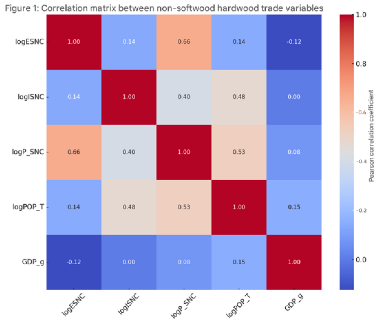
Figure 2. Projection of countries into the factorial plan.

Figure 2. Projection of countries into the factorial plan.

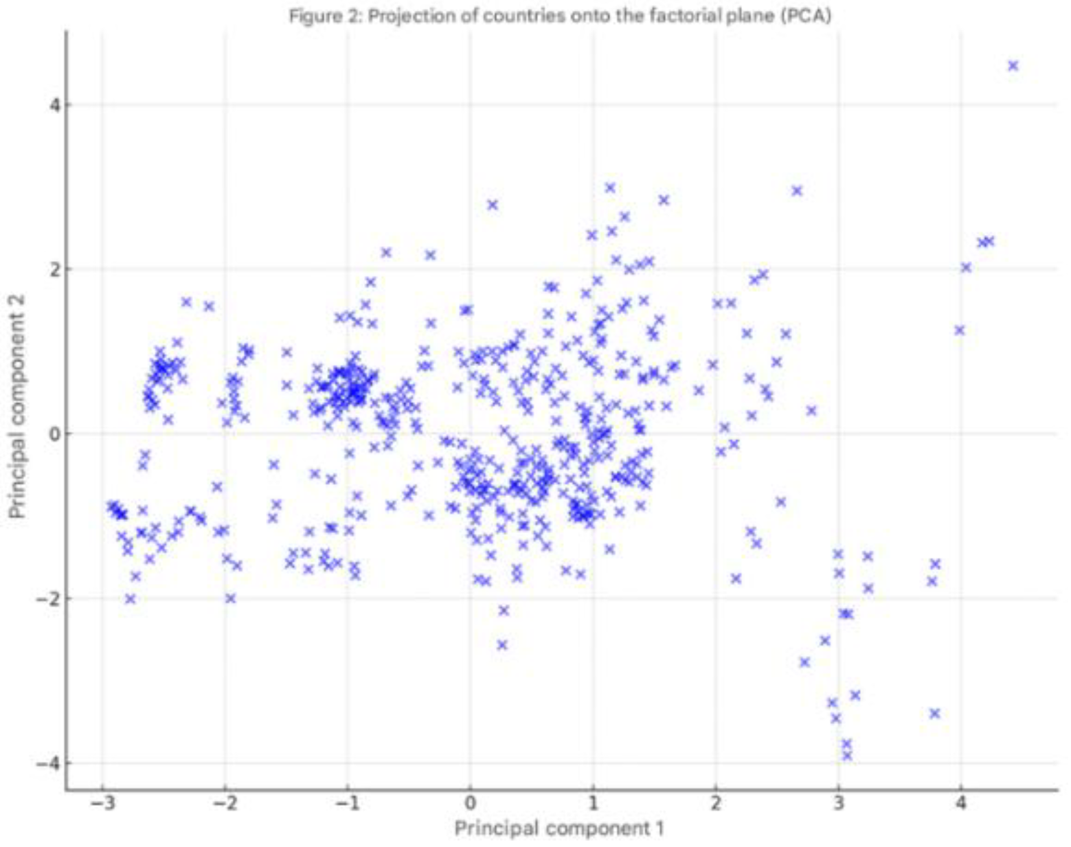
• Axis 2 (25.9% of variance):

This secondary factor is dominated by GDP growth (GDP_g), which appears to vary independently of the other trade dimensions. Projection onto the factorial plane shows a clear distinction between tropical producing countries (more to the left of the F1 axis) and importing countries (to the right of F1), confirming the results of the CAH typology.

These results highlight an asymmetrical pattern of trade in non-coniferous hardwood, in which tropical African countries appear as suppliers, and the major demographic powers (Asia and the West) as the main consumers. The influence of population on import volumes confirms the role of demographics as a driver of demand, while the absence of a strong link with GDP growth suggests that the timber trade remains dependent on structural (resources, industry, logistics) rather than cyclical logics.

4.1.3. Typological Analysis (Hierarchical Ascending Classification)

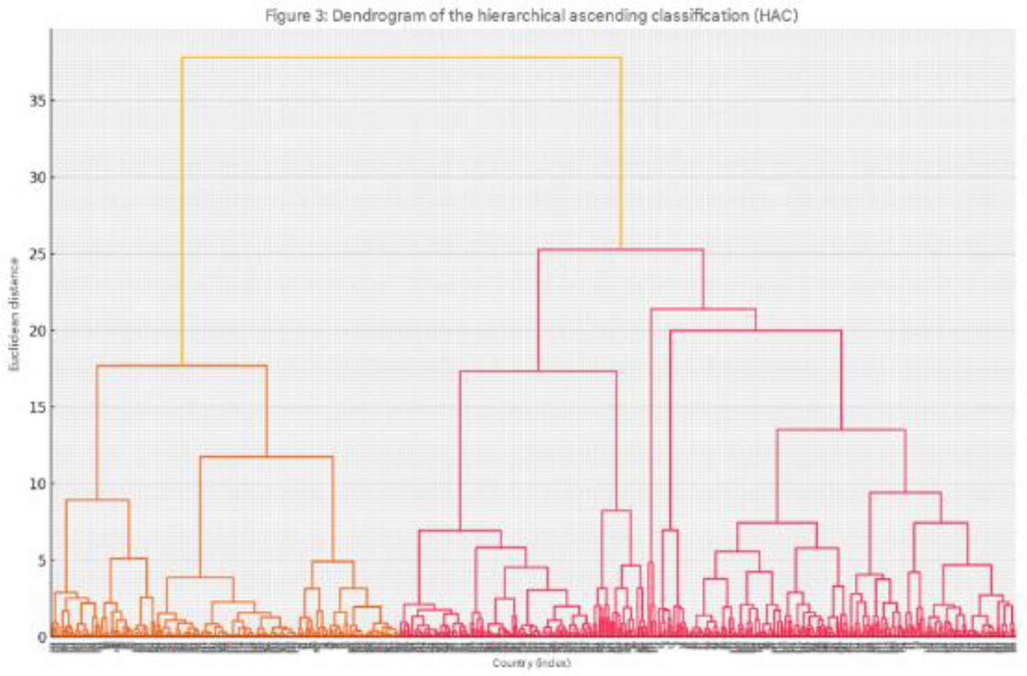
Hierarchical Ascending Classification (HAC) applied to standardized data has enabled us to group countries into four distinct types:

• Group 1: Producer-exporters: These countries, like Gabon and Congo, have high production (logP_SNC) and high exports (logESNC), but a lower population (logPOP_T), reflecting an outward focus. Brazil, on the other hand, has a large population but low domestic consumption, due to low industrialization, low average income and other internal factors.
• Group 2: Importers with large populations: This group includes countries such as China and India, characterized by strong domestic demand, reflected in high imports (logISNC) and a very large population.
• Group 3: Players with little commercial involvement: Countries such as Angola and Cameroon appear here, with low production, import and export volumes. This group is often linked to economic instability or a lack of integration into international timber trade circuits.
• Group 4: Import-export countries group: Import-export countries play a key role in the global flow of tropical sawnwood. They import raw materials (logs or rough sawn timber) for processing, storage or re-export to other markets, often with added value. Mainly made up of the USA, Germany, the Netherlands, Belgium, Vietnam, France and Singapore. Importing and re-exporting countries are essential but controversial links in the flow of tropical sawnwood. Their role enables efficient market globalization, but also accentuates the risks of illegal deforestation and value capture to the detriment of producer countries.

Figure 3. Dendrogram of the hierarchical ascending classification (HAC).

Figure 3. Dendrogram of the hierarchical ascending classification (HAC).

4.2. Dynamic Analysis of the Effects of Non-Coniferous Hardwood Exports

4.2.1. Descriptive Analysis in N and Large T Panels

The descriptive analysis provides a detailed interpretation of the international trade in non-coniferous timber. The analysis is structured according to the sections and what each test brings to the large N and T panel study. Table 3 summarizes the characteristics of the panel variables:

Table 3. Characteristics of panel variables.

Variable	Average (total standard deviation)	Standard deviation between (cross-sectional)	Intra standard deviation (over time)
ESNCit	256 260.4 (527 390,4)	527 390.4	204 238.6
P_SNCit	2 061 532 (5 304 556)	5 304 556	2 978 146
ISNCit	341 003.7 (1 011 724)	1 011 724	498 396,1
POP_Tit	100M (272M)	272M	24.3M
GDP_git	5.38 % (14.02 %)	14.02 %	3.97 %

Table 3. Characteristics of panel variables.

Variable	Average (total standard deviation)	Standard deviation between (cross-sectional)	Intra standard deviation (over time)
ESNCit	256 260.4 (527 390,4)	527 390.4	204 238.6
P_SNCit	2 061 532 (5 304 556)	5 304 556	2 978 146
ISNCit	341 003.7 (1 011 724)	1 011 724	498 396,1
POP_Tit	100M (272M)	272M	24.3M
GDP_git	5.38 % (14.02 %)	14.02 %	3.97 %

Interpretation: Standard deviations between (cross-sectional) are very high, especially for production and imports, suggesting considerable heterogeneity between countries. Intra standard deviations (within/time variation) are also high, indicating significant evolutions over time. GDP growth varies little over time, but varies more between countries. Exports are relatively stable compared to production, but remain highly dispersed across countries.

4.2.2. Cross-Sectional Dependence (CSD) test

Several tests here for variable logs (logESNC, logISNC, etc.).

Table 4. Cross-sectional dependence test for variables of interest.

Variable	CD	CDw	CDw+	CSD
Log (ESNCit)	9.17 (0.000)	-2.62 (0.009)	2627.31 (0.000)	6.71 (0.000)
Log (P_SNCit)	10.47 (0.000)	-1.71 (0.087)	3462.08 (0.000)	6.35 (0.000)
Log (ISNCit)	-1.83 (0.067)	-1.82 (0.069)	3654.34 (0.000)	-0.99 (0.324)
Log (POP_Tit)	66.13 (0.000)	-2.93 (0.003)	7270.86 (0.000)	-1.25 (0.211)
GDP_git	78.51 (0.000)	1.63 (0.104)	3296.22 (0.000)	-2.70 (0.007)

Table 4. Cross-sectional dependence test for variables of interest.

Variable	CD	CDw	CDw+	CSD
Log (ESNCit)	9.17 (0.000)	-2.62 (0.009)	2627.31 (0.000)	6.71 (0.000)
Log (P_SNCit)	10.47 (0.000)	-1.71 (0.087)	3462.08 (0.000)	6.35 (0.000)
Log (ISNCit)	-1.83 (0.067)	-1.82 (0.069)	3654.34 (0.000)	-0.99 (0.324)
Log (POP_Tit)	66.13 (0.000)	-2.93 (0.003)	7270.86 (0.000)	-1.25 (0.211)
GDP_git	78.51 (0.000)	1.63 (0.104)	3296.22 (0.000)	-2.70 (0.007)

• Interpretation:

Most CD tests are significant, indicating cross-sectional dependence (CSD). This means that shocks or developments in one country influence other countries. This is common in trade models (interdependence via trade).

• Variables such as logESNC and logISNC clearly show a strong CSD.
• The logP_SNC variable is less affected (non-significant at 5% on several tests), suggesting more independent behavior.

Conclusion: CSD is present → we need to use estimators robust to this dependence, such as those by Pesaran or Westerlund.

4.2.3. Slope Heterogeneity Test

Table 5. Multiple slope heterogeneity tests.

Test	Statistics	p-value	Adjusted statistics	Adjusted p-value
Pesaran-Yamagata (CSA)	1.327	0.185	2.064	0.039
PY (AR adjusted)	2.807	0.005	3.285	0.001
Blomquist & Westerlund	2.807	0.005	3.285	0.001
PY (Single)	-7.222	0.000	2.319	0.020

Table 5. Multiple slope heterogeneity tests.

Test	Statistics	p-value	Adjusted statistics	Adjusted p-value
Pesaran-Yamagata (CSA)	1.327	0.185	2.064	0.039
PY (AR adjusted)	2.807	0.005	3.285	0.001
Blomquist & Westerlund	2.807	0.005	3.285	0.001
PY (Single)	-7.222	0.000	2.319	0.020

• Interpretation:

The tests reveal significant slope heterogeneity in the panel data, indicating that the relationships between explanatory variables and exports, for instance, differ substantially from one country to another. This is a critical feature in large-N panels and justifies the use of variable-coefficient models, such as heterogeneous fixed-effects models or MG and CCEMG estimators. The findings support the application of both static and dynamic modeling in wide panels, based on several key elements: first, the strong heterogeneity across countries, as evidenced by descriptive statistics and heterogeneity tests; second, the presence of significant cross-sectional dependence, which calls for robust estimators like Driscoll-Kraay or Pesaran’s CCE approach. Furthermore, the data exhibit marked dynamic behavior, which justifies the inclusion of lagged terms in the models, in line with dynamic panel specifications. Lastly, the considerable intra- and inter-country variation underscores the necessity of incorporating fixed or variable effects over time and across countries.

4.2.4. Summary of Preliminary Statistical Analysis for the Dynamics of Non-Coniferous Hardwood Export Effects

Descriptive analysis of the data reveals considerable heterogeneity between ITTO member countries in terms of exports, production and imports of sawn non-coniferous timber. The high standard deviations between countries (e.g. 5,304,556 m³ for production) reflect marked structural differences in industrial capacities and trade dynamics. In addition, significant temporal variations, particularly within exports and imports, underline the need to model these data using dynamic approaches.

The results of cross-sectional dependence tests (CSD) reveal significant interdependence between countries for the model's main variables (exports, imports, GDP growth, etc.), confirmed by significant CD, CDw+ and CD* statistics at conventional thresholds (p < 0.01). This dependence can be explained by trade or macroeconomic spillover effects, reinforcing the need to use estimators robust to CSD, such as Common Correlated Effects (CCE) or Driscoll-Kraay.

Furthermore, tests for slope heterogeneity (Pesaran-Yamagata, Blomquist-Westerlund) show highly significant p-values (< 0.05), indicating that coefficients vary substantially from country to country. Thus, the relationships between macroeconomic determinants and timber trade flows cannot be assumed to be homogeneous. This characteristic justifies the use of panel models with heterogeneous coefficients, such as Mean Group (MG) or Pooled Mean Group (PMG), to better capture the structural diversity of trade behavior within the panel.

4.2.5. Stationarity Tests (Unit Root)

In order to verify the stationarity properties of the series used in the dynamic modeling of non-coniferous sawnwood exports, several unit root tests adapted to panel data were applied: the PESCADF test and the Fisher-ADF test.

4.2.5.1. PESCADF Test Results

Table 6 of the PESCADF test shows that, for all variables except GDP growth (GDP_g), the Z[t-bar] statistics at level are positive and insignificant (p-values > 0.05), indicating non-stationarity at level.

At first difference, all variables, including GDP_g, become significant with zero p-values, suggesting that they become stationary after differentiation. This shows that the logESNC, logP_SNC, logISNC, logPOP_T, and GDP_g series are integrated of order 1, i.e. I (1).

4.2.5.2. Fisher Test Results (ADF)

The results of the Fisher test (ADF) confirm the above findings. Using the P, Z and L* statistics at level, the p-values are generally insignificant (e.g. logISNC and logPOP_T have p-values of 0.436 and 1.000 respectively).

Table 7. Test de Fisher (ADF).

Statistics			Variable independent
			Log (ESNCit)	Log (P_SNCit)	Log (ISNCit)	Log (POP_Tit)	Log (GDP_git)
P	Level	Statistic	213.348	167.903	117.801	6.9392	139.972
		p-value	0.000	0.001	0.436	1.000	0.064
	First diference	Statistic	283.441	284.803	329.185	245.620	490.484
		p-value	0.000	0.000	0.000	0.000	0.000
Z	Level	Statistic	-2.7162	-2.153	1.597	12.0549	-2.0567
		p-value	0.0033	0.0157	0.9449	1.000	0.0199
	First diference	Statistic	-9.0499	-7.732	-10.158	-8.9184	-14.502
		p-value	0.000	0.000	0.000	0.000	0.000
L*	Level	Statistic	-3.5572	-2.7288	1.5959	11.842	-2.0207
		p-value	0.0002	0.0034	0.9442	1.000	0.0221
	First diference	Statistic	-9.2656	-8.5826	-10.854	-8.3583	-17.239
		p-value	0.000	0.000	0.000	0.000	0.000
Pm	Level	Value	6.391	3.407	0.118	-7.160	1.573
		p-value	0.000	0.0003	0.4529	1.000	0.0578
	First diference	Value	-9.265	11.082	13.996	8.51	24.586
		p-value	0.000	0.000	0.000	0.000	0.000

Table 7. Test de Fisher (ADF).

Statistics			Variable independent
			Log (ESNCit)	Log (P_SNCit)	Log (ISNCit)	Log (POP_Tit)	Log (GDP_git)
P	Level	Statistic	213.348	167.903	117.801	6.9392	139.972
		p-value	0.000	0.001	0.436	1.000	0.064
	First diference	Statistic	283.441	284.803	329.185	245.620	490.484
		p-value	0.000	0.000	0.000	0.000	0.000
Z	Level	Statistic	-2.7162	-2.153	1.597	12.0549	-2.0567
		p-value	0.0033	0.0157	0.9449	1.000	0.0199
	First diference	Statistic	-9.0499	-7.732	-10.158	-8.9184	-14.502
		p-value	0.000	0.000	0.000	0.000	0.000
L*	Level	Statistic	-3.5572	-2.7288	1.5959	11.842	-2.0207
		p-value	0.0002	0.0034	0.9442	1.000	0.0221
	First diference	Statistic	-9.2656	-8.5826	-10.854	-8.3583	-17.239
		p-value	0.000	0.000	0.000	0.000	0.000
Pm	Level	Value	6.391	3.407	0.118	-7.160	1.573
		p-value	0.000	0.0003	0.4529	1.000	0.0578
	First diference	Value	-9.265	11.082	13.996	8.51	24.586
		p-value	0.000	0.000	0.000	0.000	0.000

• However, at first difference, all statistics become highly significant (p < 0.01), indicating stationarity of the series after differentiation. This consistency between tests justifies the first-difference approach for subsequent dynamic analyses.

4.2.6. Cointegration Tests

Confirmation of the order of integration of the variables enables us to examine the existence of a cointegrating relationship between exports of non-coniferous sawn timber (logESNC) and the explanatory variables. Two types of test are used: the Westerlund test and the combined Westerlund & Pedroni test.

4.2.6.1. Westerlund Test Results (ECM)

The results of Westerlund's ECM test (see Table 8) reveal that several forms of the test (Gt, Pt, Ga, Pa) detect a cointegrating relationship for the explanatory variables logP_SNC, logISNC, logPOP_T and GDP_g:

The Gt and Pt statistics are highly significant for all variables (p < 0.01), indicating the presence of a long-term adjustment mechanism in the export equation. The Ga test reveals strong significance for the variable logP_SNC (p = 0.000), suggesting a consistent long-run relationship for this variable across countries; however, it is not significant for others, such as logISNC (p = 0.782), pointing to possible heterogeneity in long-term dynamics among countries. Additionally, while most Pa values are statistically significant, the exception is logPOP_T, which has a p-value of 0.371, indicating a potential absence of cointegration between population and exports in certain countries. Taken together, these results support the existence of a stable long-run relationship between exports and key explanatory variables, particularly domestic production, imports, and economic growth.

4.2.6.2. Westerlund and Pedroni Combined Test

The combined results provide further support for the existence of cointegration:

Table 9. Westerlund and Pedroni combined test.

Tests	Statistics	Values	p-value
Westerlund test for cointegration	Variance ratio	-2.0431	0.0205
Pedroni test for cointegration	Modified Phillips-Perron t	4.0429	0.000
	Phillips-Perron t	-7.0769	0.000
	Augmented Dickey-Fuller t	-6.4662	0.000

Table 9. Westerlund and Pedroni combined test.

Tests	Statistics	Values	p-value
Westerlund test for cointegration	Variance ratio	-2.0431	0.0205
Pedroni test for cointegration	Modified Phillips-Perron t	4.0429	0.000
	Phillips-Perron t	-7.0769	0.000
	Augmented Dickey-Fuller t	-6.4662	0.000

The Westerlund variance ratio test yields a significant result (p = 0.0205), confirming the existence of a long-term relationship between the variables. Additionally, all three versions of the Pedroni test—Modified Phillips-Perron, Phillips-Perron t, and ADF t—are significant at the 1% level, providing strong evidence of cointegration among the variables in the export model. Stationarity analyses show that all series are integrated of order one (I(1)), while the consistent outcomes of the cointegration tests further confirm the presence of stable long-run relationships between non-coniferous sawnwood exports (linked to processing) and key economic explanatory variables. These findings support the appropriateness of employing a long-term dynamic panel model—such as PMG, DOLS, or CCE—to analyze international timber trade among ITTO member countries.

4.2.7. Estimates

4.2.7.1. Estimates of Export Determinants from the Dynamic Models ARDL_PMG, ARDL_FE, NoCS_ARDL_CCE and CS_ARDL_CCE

Table 10. Dynamic model estimates.

VARIABLES	NoCS_ARDL_CCE	CS_ARDL_CCE (Optimal)	ARDL_PMG	ARDL_FE
Dependente variable (logESNC)
LD.logESNC	-0.078**	-0.106***
	(0.039)	(0.035)
Short-run effects
D.logP_SNC	0.066 (0.130)	0.120 (0.093)	0.115 (0.078)	0.208*** (0.074)
LD.logP_SNC	0.286** (0.129)	0.261** (0.117)
D.logISNC	0.269*** (0.058)	0.333*** (0.061)	0.257*** (0.046)	0.117*** (0.022)
LD.logISNC	0.042 (0.049)	0.072 (0.049)
D.logPOP_T			-5.923 (7.097)	-0.014 (0.043)
D.GDP_g	0.016** (0.008)	0.011* (0.007)	0.001 (0.005)	0.005 (0.006)
LD.GDP_g	-0.001 (0.006)	0.005
		(0.005)
Constant		0.011(0.020)	-4.802*** (0.473)	2.098*** (0.625)
Long-run effects
Adjust. Term (lr_logESNC)	(-)1.078*** 0.000	-1.106*** (0.035)	-0.336*** (0.026)	-0.392*** (0.021)
lr_logP_SNC	0.360*** (0.132)	0.380*** (0.111)	0.001 (0.005)	0.378*** (0.108)
lr_logISNC	0.286*** (0.071)	0.365*** (0.076)	-0.001 (0.022)	-0.001 (0.049)
lr_logPOP_T	1.201*** (0.322)	1.287*** (0.188)	1.389*** (0.210)	0.041 (0.054)
lr_GDP_g	0.003 (0.013)	0.011	0.016** (0.008)	-0.019
		(0.010)		(0.019)
lr__cons		0.019 (0.015)	-4.802*** (0.473)	2.098*** (0.625)
Comments (N/T)	1,507 (58/26)	1,507 (58/26)	1,565 (58/26)	1,565 (58/26)
CD-Statistic (residual)	-1.48	0.72	1.16	0.47
PESCADF (P)	(-)13.468***	14.013***	5.61***	7.818***
ADF-Fisher	387.821***	340.2267***	409.0523***	414.126***

Standard errors in parentheses, *** p<0.01, ** p<0.05, * p<0.1.

Table 10. Dynamic model estimates.

VARIABLES	NoCS_ARDL_CCE	CS_ARDL_CCE (Optimal)	ARDL_PMG	ARDL_FE
Dependente variable (logESNC)
LD.logESNC	-0.078**	-0.106***
	(0.039)	(0.035)
Short-run effects
D.logP_SNC	0.066 (0.130)	0.120 (0.093)	0.115 (0.078)	0.208*** (0.074)
LD.logP_SNC	0.286** (0.129)	0.261** (0.117)
D.logISNC	0.269*** (0.058)	0.333*** (0.061)	0.257*** (0.046)	0.117*** (0.022)
LD.logISNC	0.042 (0.049)	0.072 (0.049)
D.logPOP_T			-5.923 (7.097)	-0.014 (0.043)
D.GDP_g	0.016** (0.008)	0.011* (0.007)	0.001 (0.005)	0.005 (0.006)
LD.GDP_g	-0.001 (0.006)	0.005
		(0.005)
Constant		0.011(0.020)	-4.802*** (0.473)	2.098*** (0.625)
Long-run effects
Adjust. Term (lr_logESNC)	(-)1.078*** 0.000	-1.106*** (0.035)	-0.336*** (0.026)	-0.392*** (0.021)
lr_logP_SNC	0.360*** (0.132)	0.380*** (0.111)	0.001 (0.005)	0.378*** (0.108)
lr_logISNC	0.286*** (0.071)	0.365*** (0.076)	-0.001 (0.022)	-0.001 (0.049)
lr_logPOP_T	1.201*** (0.322)	1.287*** (0.188)	1.389*** (0.210)	0.041 (0.054)
lr_GDP_g	0.003 (0.013)	0.011	0.016** (0.008)	-0.019
		(0.010)		(0.019)
lr__cons		0.019 (0.015)	-4.802*** (0.473)	2.098*** (0.625)
Comments (N/T)	1,507 (58/26)	1,507 (58/26)	1,565 (58/26)	1,565 (58/26)
CD-Statistic (residual)	-1.48	0.72	1.16	0.47
PESCADF (P)	(-)13.468***	14.013***	5.61***	7.818***
ADF-Fisher	387.821***	340.2267***	409.0523***	414.126***

Standard errors in parentheses, *** p<0.01, ** p<0.05, * p<0.1.

4.2.7.2. Residual Cross-Sectional Dependency Test (CD Test)

Table 11 presents a clear and structured interpretation of the results of the cross-sectional dependence (CD) test applied to several dynamic models in a panel context with large N and T, based on the various test statistics reported:

• Interpretation of the residual cross-sectional dependency test (CD test)

The aim of these tests is to check whether there is any dependency between cross-section units (i.e., between countries, regions, etc.), which is essential in dynamic panels, especially when unobserved common shocks can bias estimates if not taken into account. Several versions of the test are used here to reinforce the robustness of the diagnosis:

• Interpretation by Model (Optimal Model CS_ARDL_CCE):

The CS_ARDL_CCE model reveals a strong cross-sectional dependence, as indicated by the CD statistic (12.28, p = 0.000). Also, the CDw test detect such dependence (2.09, p = 0.037), while the CDw+ statistic shows extremely high values (1707.99, p = 0.000), highlighting strong dependence even at low intensity levels. However, while this specification captures a substantial share of cross-sectional dependence, the results of the advanced CD* test (-1.64, p = 0.101) suggest the absence of significant cross-sectional dependence once common correlated effects are integrated into the model. This outcome supports the suitability of the CS_ARDL_CCE approach, which explicitly controls for such common factors, while underlining the importance of maintaining caution regarding potential residual dependence structures within the dataset.

NoCS_ARDL_CCE Model: All tests detect cross-sectional dependence. However, the CDw test fails to identify any, which may suggest that the number of principal components used in the model was insufficient to fully capture the underlying dependency structure.

ARDL_PMG and ARDL_FE Models: These models exhibit very strong cross-sectional dependence according to all classical tests, including CD*. Since they do not incorporate any correction for cross-dependence, the reliability of their results is questionable and may be compromised by bias.

Overall Interpretation: All estimated models exhibit some degree of cross-sectional dependence, including those employing the CCE approach specifically designed to mitigate such effects. However, the CS_ARDL_CCE model demonstrates superior robustness, revealing no evidence of residual dependence according to the advanced CD* test (-1.64; p = 0.101). These findings underscore the critical importance of accounting for common shocks and unobserved heterogeneity in dynamic panel data analysis. They also highlight the necessity of combining both conventional and robust testing procedures to ensure the absence of cross-sectional dependence bias, particularly in large panel datasets with high N and T dimensions.

4.2.7.3. Justification for Choosing the Optimal Model: CS_ARDL_CCE

When analyzing the determinants of non-coniferous timber exports in ITTO member countries, as measured by the dependent variable log (ESNC), the selection of the optimal estimation model is a key methodological issue. Among the various dynamic models assessed, the CS_ARDL_CCE model (Auto-Regressive Distributed Lag with Common Correlated Effects and slope heterogeneity) proved to be the most suitable for panels with both a large number of countries (N) and time periods (T). To validate this choice, several cross-sectional dependence tests were applied to the residuals of the estimated models in order to detect unobserved correlations across countries that, if ignored, could bias the results. The findings, summarized in Table 11, are interpreted using four complementary metrics: the classical Pesaran CD test, the robust CDw test proposed by Juodis and Reese (2021), its CDw+ extension by Fan et al. (2015), and the CD* test by Pesaran and Xie (2021), which incorporates principal component analysis (PCA) within the CCE framework.

The CS_ARDL_CCE model produces results in line with theoretical expectations. First, Pesaran’s CD test (12.28, p < 0.01) reveals the presence of significant cross-sectional dependence. Similarly, the CDw test (2.09, p = 0.037), which is better suited for dynamic panels, also detects this dependence, suggesting that the dynamic specification does not fully absorb the cross-sectional correlations. Furthermore, the CDw+ statistic (1707.99, p < 0.01), designed to capture even weak cross-sectional dependencies, confirms the persistence of such dependence within the dataset. However, the advanced CD* test (-1.64, p = 0.101), which adjusts for common correlated effects extracted via PCA (with four components retained), indicates the absence of significant residual cross-sectional dependence. These results validate the relevance of the CS_ARDL_CCE approach in explicitly controlling for unobserved common factors, while emphasizing the need to remain vigilant regarding potential remaining dependence structures.

These results show that, despite the partial control provided by the CCE approach, some residual cross-sectional dependence remains—likely due to unobserved common shocks or persistent structural linkages among countries. In comparison, the other models tested (NoCS_ARDL_CCE, ARDL_PMG, and ARDL_FE) display even higher levels of cross-sectional dependence, even under configurations intended to address these biases, thus casting doubt on the reliability of their estimates in this context.

Therefore, the CS_ARDL_CCE model emerges as the optimal choice for this study because it (i) accounts for structural heterogeneity across countries through country-specific slope coefficients, (ii) incorporates cross-sectional dependence using the Common Correlated Effects (CCE) method, and (iii) enables the joint estimation of short-run dynamics, long-run relationships, and the adjustment mechanism toward equilibrium. In sum, this model offers a robust empirical framework for analyzing the structural and dynamic drivers of non-coniferous timber exports across a wide panel while minimizing the risk of biased inferences arising from cross-sectional dependence.

4.2.7.4. Detailed Interpretation of Results (Model CS_ARDL_CCE)

Table 12. Dependent variable: log (ESNC).

Short-term effects (short-run)
Explanatory variable	Coefficient	Interpretation
ΔlogP_SNC (Production)	0.120 (ns)	Positive effect, but not significant. In the short term, a one-off increase in local non-coniferous tropical hardwood lumber production (processing) has no statistically assured effect on exports.
ΔlogISNC (Imports)	0.333*	Highly significant. In the short term, a 1% increase in imports of non-coniferous sawnwood leads to a 0.33% increase in exports. This could suggest a logic of local processing and re-export or a matching effect between local and imported supply.
ΔGDP_g (GDP growth)	0.011*	Significant at the 10% level. Stronger economic growth slightly boosts exports in the short term (+1% GDP → +1.1% exports). This could reflect an improvement in logistics capacities or a growing global demand effect.
ns: not significant.
Effect of adjustment towards equilibrium
Term	Coefficient	Interpretation
Adjustment Term (lr_logESNC)	-1.106***	The adjustment term associated with the lagged dependent variable is very significant and negative at 1% (-1.106***, standard deviation: 0.035), indicating a high speed of convergence to the long-term equilibrium after a shock. This suggests strong resilience of the exporting economic system in the medium term.
Long-run effects
Explanatory variable	Coefficient	Interpretation
lr_logP_SNC	0.380***	Highly significant. A 1% increase in national production of non-coniferous hardwood sawn timber leads to a 0.38% increase in long-term exports. This validates a positive structural relationship between local production and export performance.
lr_logISNC	0.365***	Also, highly significant. The effect is strong: 1% more imports leads to 0.37% more exports in the long term. This confirms vertical commercial integration in the non-coniferous wood sector.
lr_logPOP_T	1.287***	Here it is highly significant: an increase in total population is positively associated with exports in the long term. This may indicate a structural development effect: the larger a country's population, the more it develops commercial and productive infrastructures.
lr_GDP_g	0.011 (ns)	Not significant in the long term. Economic growth does not appear to have a structural effect on long-term exports in this sector.
Constant (lr_cons)	0.019 (ns)	No significant long-term effect of the constant.
ns: not significant

Table 12. Dependent variable: log (ESNC).

Short-term effects (short-run)
Explanatory variable	Coefficient	Interpretation
ΔlogP_SNC (Production)	0.120 (ns)	Positive effect, but not significant. In the short term, a one-off increase in local non-coniferous tropical hardwood lumber production (processing) has no statistically assured effect on exports.
ΔlogISNC (Imports)	0.333*	Highly significant. In the short term, a 1% increase in imports of non-coniferous sawnwood leads to a 0.33% increase in exports. This could suggest a logic of local processing and re-export or a matching effect between local and imported supply.
ΔGDP_g (GDP growth)	0.011*	Significant at the 10% level. Stronger economic growth slightly boosts exports in the short term (+1% GDP → +1.1% exports). This could reflect an improvement in logistics capacities or a growing global demand effect.
ns: not significant.
Effect of adjustment towards equilibrium
Term	Coefficient	Interpretation
Adjustment Term (lr_logESNC)	-1.106***	The adjustment term associated with the lagged dependent variable is very significant and negative at 1% (-1.106***, standard deviation: 0.035), indicating a high speed of convergence to the long-term equilibrium after a shock. This suggests strong resilience of the exporting economic system in the medium term.
Long-run effects
Explanatory variable	Coefficient	Interpretation
lr_logP_SNC	0.380***	Highly significant. A 1% increase in national production of non-coniferous hardwood sawn timber leads to a 0.38% increase in long-term exports. This validates a positive structural relationship between local production and export performance.
lr_logISNC	0.365***	Also, highly significant. The effect is strong: 1% more imports leads to 0.37% more exports in the long term. This confirms vertical commercial integration in the non-coniferous wood sector.
lr_logPOP_T	1.287***	Here it is highly significant: an increase in total population is positively associated with exports in the long term. This may indicate a structural development effect: the larger a country's population, the more it develops commercial and productive infrastructures.
lr_GDP_g	0.011 (ns)	Not significant in the long term. Economic growth does not appear to have a structural effect on long-term exports in this sector.
Constant (lr_cons)	0.019 (ns)	No significant long-term effect of the constant.
ns: not significant

The estimation of the optimal dynamic model, CS_ARDL_CCE, provided a fine-grained reading of the determinants of non-coniferous hardwood lumber exports (logESNC) in a heterogeneous panel framework with cross-dependencies. By combining short- and long-term dynamic effects with structural specificities between countries, this model proved particularly well-suited to the characteristics of the data observed.

• Short-term effects

Analysis of the short-term coefficients highlights several key results. Firstly, the effect of variation in local non-coniferous wood production (ΔlogP_SNC) appears positive but insignificant, suggesting that a one-off increase in domestic supply does not immediately translate into an increase in exports. On the other hand, imports (ΔlogISNC) show a significant and positive effect: a 1% increase in imports is associated with a 0.33% increase in exports in the short term. This result could reflect local processing for re-export or a complementarity effect between local and imported wood. Finally, economic growth (ΔGDP_g) exerts a slightly significant effect: a 1% growth in GDP leads to an increase of around 1.1% in exports, which could be explained by an improvement in logistics infrastructures or increased global demand.

• Adjustment towards balance

The adjustment term associated with the lagged dependent variable is very significant and negative at 1% (-1.106***, standard deviation: 0.035), indicating a high speed of convergence to the long-term equilibrium after a shock. This suggests strong resilience of the exporting economic system in the medium term.

• Long-term effects

Long-term results reveal robust structural relationships. Domestic non-coniferous wood production (logP_SNC) is positively and significantly related to exports (+0.38%), confirming that a sustained increase in production translates into better export performance. Similarly, imports (logISNC) maintain a significant effect (+0.37%), supporting the hypothesis of vertical integration of the sector on an international scale. Total population (logPOP_T), which is only significant in this model, has a significant effect (+1.29%), suggesting that broader demographic structures are correlated with greater trade capacity. On the other hand, neither long-term economic growth (GDP_g) nor the constant show significant effects in this framework.

• Interpretation in the light of descriptive statistics

The data show strong heterogeneity between countries, particularly in terms of production and export volumes, which fully justifies the use of a model like CS_ARDL_CCE, capable of capturing these differences. Furthermore, the low intra-temporal variability of the series reinforces the relevance of the ARDL framework, in which the slow adjustment dynamic (10% per year) proves consistent with observed reality. The results obtained from the CS_ARDL_CCE model are both economically consistent and statistically robust. They highlight the importance of structural factors such as local production and imports in export performance in the long term, while GDP exerts mainly a marginal effect in the short term. In this sense, policies aimed at strengthening processing capacities and improving logistics chains appear to be strategic levers for supporting sustainable exports of non-coniferous wood.

4.2.8. Testing for Granger Causality

4.2.8.1. Test for Granger Non-Causality in Heterogeneous Panel Data Models

Table 13. Granger non-causality in heterogeneous panel data models.

Variables	(HPJ_Bootstrap)
L.logP_SNC	-0.004 (0.063)
L.logPOP_T	-0.979** (0.442)
L.GDP_g	-0.012* (0.006)
L.logISNC	-0.077* (0.039)
Comments (N/T)	1,623 (58/26)
HPJ Wald test :	16.5364
p-value	0.0024

Standard in parentheses, *** p<0.01, ** p<0.05, * p<0.1.

Table 13. Granger non-causality in heterogeneous panel data models.

Variables	(HPJ_Bootstrap)
L.logP_SNC	-0.004 (0.063)
L.logPOP_T	-0.979** (0.442)
L.GDP_g	-0.012* (0.006)
L.logISNC	-0.077* (0.039)
Comments (N/T)	1,623 (58/26)
HPJ Wald test :	16.5364
p-value	0.0024

Standard in parentheses, *** p<0.01, ** p<0.05, * p<0.1.

• Interpreting the Granger non-causality test (HPJ and Dumitrescu & Hurlin)

Table 14. HPJ test results (Het Panel Joint Test - Bootstrap).

Explanatory variable (lagged)	Coefficient	Error-SD	Interpretation
L.logP_SNC (Production)	-0.004	0.063	Trend towards a marginally significant unidirectional relationship towards ESNC. In other words, past production has little influence on current exports.
L.logPOP_T (Population)	-0.979**	0.044	Significant effect: past population causes Granger exports. This reinforces the idea of a structural development effect.
L.GDP_g (GDP)	-0.012*	0.006	Significant effect at 10%: past economic growth has a causal impact on short-term exports.
L.logISNC (Imports)	-0.077*	0.039	Significant causal effect of past imports on exports. This suggests an integrated import-processing-export mechanism.

Table 14. HPJ test results (Het Panel Joint Test - Bootstrap).

Explanatory variable (lagged)	Coefficient	Error-SD	Interpretation
L.logP_SNC (Production)	-0.004	0.063	Trend towards a marginally significant unidirectional relationship towards ESNC. In other words, past production has little influence on current exports.
L.logPOP_T (Population)	-0.979**	0.044	Significant effect: past population causes Granger exports. This reinforces the idea of a structural development effect.
L.GDP_g (GDP)	-0.012*	0.006	Significant effect at 10%: past economic growth has a causal impact on short-term exports.
L.logISNC (Imports)	-0.077*	0.039	Significant causal effect of past imports on exports. This suggests an integrated import-processing-export mechanism.

HPJ Wald test overall = 16.53, p = 0.0024: the null hypothesis of no joint causality is rejected. This means that, overall, the explanatory variables (P_SNC, ISNC, GDP_g, POP_T) significantly cause exports (log ESNC) in a heterogeneous panel.

4.2.8.2. Dumitrescu & Hurlin (2012) Granger Non-Causality Test Results (Test Unidirectional)

Table 15. Dumitrescu & Hurlin (2012) Granger non-causality test results.

Causality	Z-bar	p-value	Z-bar tilde	p-value	Remarks(Test unidirectional)
ESNC-P_SNC	6.6508	0.0000	5.2666	0.0000	Bi-causal Relationship
P_SNC-ESNC	8.8025	0.0000	7.1058	0.0000
ESNC-ISNC	4.084	0.0000	3.0725	0.0021	Bi-causal Relationship
ISNC-ESNC	5.941	0.0000	4.6599	0.0000
ESNC-POP_T	7.3583	0.0000	5.8714	0.0000	Bi-causal Relationship
POP_T-ESNC	20.4345	0.0000	17.0488	0.0000
ESNC-GDP_g	5.1352	0.0000	3.971	0.0001	Bi-causal Relationship
GDP_g-ESNC	2.5862	0.0097	1.7922	0.0731

Table 15. Dumitrescu & Hurlin (2012) Granger non-causality test results.

Causality	Z-bar	p-value	Z-bar tilde	p-value	Remarks(Test unidirectional)
ESNC-P_SNC	6.6508	0.0000	5.2666	0.0000	Bi-causal Relationship
P_SNC-ESNC	8.8025	0.0000	7.1058	0.0000
ESNC-ISNC	4.084	0.0000	3.0725	0.0021	Bi-causal Relationship
ISNC-ESNC	5.941	0.0000	4.6599	0.0000
ESNC-POP_T	7.3583	0.0000	5.8714	0.0000	Bi-causal Relationship
POP_T-ESNC	20.4345	0.0000	17.0488	0.0000
ESNC-GDP_g	5.1352	0.0000	3.971	0.0001	Bi-causal Relationship
GDP_g-ESNC	2.5862	0.0097	1.7922	0.0731

4.2.8.3. Results of the Granger Test by Dumitrescu & Hurlin (2012), (Bi-Directional)

This test explores two-way causality and significance across panel units.

Table 16. Granger test from Dumitrescu & Hurlin (2012), (bi-directional).

Relationship tested	Z-bar (p-value)	Z-tilde (p-value)	Interpretation
ESNC ↔ P_SNC	6.65 ↔ 8.80	0.0000	Very strong two-way causality between local production and exports: one influences the other. This confirms the dynamic adjustment logic of the ARDL model.
ESNC ↔ ISNC	4.08 ↔ 5.94	0.0000	The relationship is also bidirectional: exports react to imports and vice versa. This reinforces the idea of an integrated "import-processing-export" cycle.
ESNC ↔ POP_T	7.36 ↔ 20.43	0.0000	Very strong bilateral relationship: demographic weight affects exports and vice versa. This suggests a structural link between population growth and export specialization.
ESNC ↔ GDP_g	5.14 ↔ 2.58	0.0001 0.0097	Bilateral relationship, but less strong on the GDP → export side. This confirms the ARDL results: GDP has only a marginal long-term role in explaining exports.

Table 16. Granger test from Dumitrescu & Hurlin (2012), (bi-directional).

Relationship tested	Z-bar (p-value)	Z-tilde (p-value)	Interpretation
ESNC ↔ P_SNC	6.65 ↔ 8.80	0.0000	Very strong two-way causality between local production and exports: one influences the other. This confirms the dynamic adjustment logic of the ARDL model.
ESNC ↔ ISNC	4.08 ↔ 5.94	0.0000	The relationship is also bidirectional: exports react to imports and vice versa. This reinforces the idea of an integrated "import-processing-export" cycle.
ESNC ↔ POP_T	7.36 ↔ 20.43	0.0000	Very strong bilateral relationship: demographic weight affects exports and vice versa. This suggests a structural link between population growth and export specialization.
ESNC ↔ GDP_g	5.14 ↔ 2.58	0.0001 0.0097	Bilateral relationship, but less strong on the GDP → export side. This confirms the ARDL results: GDP has only a marginal long-term role in explaining exports.

4.2.8.4. Cross-Interpretation with ARDL Results (CS_ARDL_CCE)

Table 17. Cross-interpretation with results from the CS_ARDL_CCE model.

Crossed element	Test ARDL (short / long term)	Granger (HPJ / D&H)	Integrated interpretation
Production (logP_SNC)	Short-term: NS Long-term: +0.38*	Bilateral causality (strong)	Even if the immediate effect is weak, production plays a structuring role in the evolution of exports. Bidirectional causality confirms a dynamic of interdependence.
Imports (logISNC)	Short-term: +0.33*** Long-term: +0.365***	Strong bilateral causality	Confirms the key role of imports in the export dynamic. Granger validates the economic logic: import-export flows are complementary in this sector.
Population (logPOP_T)	Long-term: +1.28***	Bilateral causality	Strong structural effect. Population is not just an explanatory factor, it also interacts dynamically with exports (effect of market size, infrastructure, etc.).
GDP growth (GDP_g)	Short-term: +0.011* Long-term: NS	Causality low but present (especially ESNC → GDP)	Supports the idea that growth has an indirect, short-term effect on exports, via improved logistics capacity or opportunity effects.

Table 17. Cross-interpretation with results from the CS_ARDL_CCE model.

Crossed element	Test ARDL (short / long term)	Granger (HPJ / D&H)	Integrated interpretation
Production (logP_SNC)	Short-term: NS Long-term: +0.38*	Bilateral causality (strong)	Even if the immediate effect is weak, production plays a structuring role in the evolution of exports. Bidirectional causality confirms a dynamic of interdependence.
Imports (logISNC)	Short-term: +0.33*** Long-term: +0.365***	Strong bilateral causality	Confirms the key role of imports in the export dynamic. Granger validates the economic logic: import-export flows are complementary in this sector.
Population (logPOP_T)	Long-term: +1.28***	Bilateral causality	Strong structural effect. Population is not just an explanatory factor, it also interacts dynamically with exports (effect of market size, infrastructure, etc.).
GDP growth (GDP_g)	Short-term: +0.011* Long-term: NS	Causality low but present (especially ESNC → GDP)	Supports the idea that growth has an indirect, short-term effect on exports, via improved logistics capacity or opportunity effects.

Granger non-causality tests conducted within a heterogeneous and dynamic panel framework further validate and complement the insights derived from the CS_ARDL_CCE model. The analysis reveals that bilateral causal relationships are predominant, especially among production, imports, and exports—an economically consistent finding for a wood value chain that relies on processing and vertical integration. Population emerges as a structurally significant variable, serving as a deep-rooted driver of export specialization. While GDP plays a comparatively less central role, it still functions as an important factor in cyclical adjustments within the export dynamics.

4.2.8.5. Analysis of Dynamic Causality: Granger Tests in Heterogeneous Panels

Dynamic causality relationships between explanatory variables and exports of sawn non-coniferous wood (logESNC) were examined using Granger tests adapted to heterogeneous panel data. Two complementary approaches were mobilized: the HPJ test (Het Panel Joint test with Bootstrap) and the test proposed by Dumitrescu and Hurlin (2012), making it possible to incorporate both individual heterogeneity and cross-sectional dependence.

The results of the HPJ test reveal an overall significance of causality, with a Wald test of 16.53 (p = 0.0024), indicating that the explanatory variables taken together (logP_SNC, logISNC, GDP_g, logPOP_T) significantly influence exports. More specifically, past GDP (GDP_g) and imports (logISNC) show significant effects at the 10% level on contemporary exports, suggesting a plausible economic link between growth, trade integration and export performance in the short term. The demographic variable (logPOP_T) shows a significant influence at 5%, reinforcing the hypothesis of a structural effect linked to the size of the domestic market. Past production (logP_SNC) shows a weakly significant effect (p = 0.063), reflecting a potentially unidirectional relationship.

The results of the Dumitrescu and Hurlin test confirm and clarify this causal dynamic by identifying significant two-way relationships. All the pairs of variables tested (ESNC ↔ P_SNC, ESNC ↔ ISNC, ESNC ↔ POP_T, ESNC ↔ GDP_g) show highly significant Z-bar and Z-tilde coefficients (p < 0.01), signaling robust bidirectional causalities. These results point to a dynamic interdependence between exports and their structural and cyclical determinants. For example, the relationship between production and exports is doubly causal, corroborating the role of an endogenous adjustment logic in forest value chains. Similarly, import flows, essentially destined for local processing, appear to be a key link in export performance.

Cross-referenced with the results of the CS_ARDL_CCE model, this analysis supports the idea that export dynamics in ITTO countries are based on a complex interaction between structural (population, production) and cyclical (growth, imports) factors, with significant short- and long-term elasticities. Economic growth, although weakly linked to exports in the long term, contributes to their dynamism in the short term via opportunity or infrastructure effects. Thus, the robustness of the causal relationships detected reinforces the economic and empirical validity of the ARDL model selected, and suggests concrete implications for development strategy and trade policy in the forestry sector.

4.3. Analysis of Structural Inequalities

4.3.1. Structural Inequalities in the International Tropical Hardwood Trade: Economic, Environmental and Geopolitical Analysis:

Empirical analysis (exploratory, descriptive and macro-econometric) of the structure of the ITTO market and the determinants of tropical hardwood exports reveals structural and functional disparities between the countries that own ecosystem services and the importing/exporting countries.) International trade in tropical hardwoods highlights these persistent structural disparities between producer countries in the South (particularly in Central Africa) and importing and re-exporting countries in the North and Asia. These imbalances, well documented in the literature (Deacon, 2020; [1,41], revolve around three interdependent dimensions: (Economic: imbalances in the distribution of the value chain), (Environmental: outsourcing of ecological impacts to producer countries) and (Geopolitics: institutional asymmetries and power relations unfavorable to exporting countries).

4.3.1.1. Economic Inequalities: Value Capture and Forest Rent

• Extractive Specialization in Producing Countries

Central African countries remain heavily specialized in the extraction and export of raw logs, limiting their ability to benefit from the broader economic gains associated with local value addition. Despite accounting for more than 15% of global tropical timber supply [1], these countries process only a small portion of their wood domestically—between 12% and 18% of volumes are sawn or otherwise transformed prior to export (World Bank, 2022). This limited local processing reflects a structural vulnerability, as evidenced by the negative correlation between GDP growth (GDP_g) and the export of unprocessed sawnwood (logESNC), with a coefficient of –0.12 (p < 0.01), suggesting that reliance on raw timber exports may hinder sustainable economic development.

Table 18. Local processing rate (%) and exports (million m³).

Country	Local processing rate (%)	Exports (million m³)
Gabon	14.2	5.3
Cameroon	11.8	3.1
Congo	17.6	2.7
Malaysia	68.5	4.9
Brazil	63.2	6.2

Source : (GFW, 2023) [35].

Table 18. Local processing rate (%) and exports (million m³).

Country	Local processing rate (%)	Exports (million m³)
Gabon	14.2	5.3
Cameroon	11.8	3.1
Congo	17.6	2.7
Malaysia	68.5	4.9
Brazil	63.2	6.2

Source : (GFW, 2023) [35].

• Downstream Domination by Re-exporting Countries

Importing countries overwhelmingly capture the majority of value added within the tropical timber value chain. For example, China processes approximately 60% of African logs into finished wood products [36], while France re-exports nearly 40% of its imported tropical timber after domestic transformation [1]. This control over downstream activities translates into substantial economic gains, as illustrated by the significant price gap: tropical hardwood furniture commands prices that are 3.5 to 4 times higher than those of raw exported logs [35,44]. This asymmetry highlights the unequal distribution of forest rent and value capture between producing and re-exporting nations.

Table 19. Price comparison by value chain stage (USD/m³).

Product	Exporting country	Re-exporting country	Average price (USD/m³)
Logs (Gabon)	Gabon	–	190
Primary sawn timber	Cameroon	France	360
Finished furniture/flooring	China (re-export)	United States	720

Source : World Bank.

Table 19. Price comparison by value chain stage (USD/m³).

Product	Exporting country	Re-exporting country	Average price (USD/m³)
Logs (Gabon)	Gabon	–	190
Primary sawn timber	Cameroon	France	360
Finished furniture/flooring	China (re-export)	United States	720

Source : World Bank.

Granger test: significant two-way causality between logESNC and logISNC (p < 0.001), indicating a circular relationship between gross exports and imports of finished products. The bar chart shows average exports (m³) of tropical non-coniferous sawnwood by country and destination (Asia vs. Europe+USA). It clearly highlights structural inequalities in trade flows:

Figure 4. Structural inequalities in the international trade of tropical hardwoods.

Figure 4. Structural inequalities in the international trade of tropical hardwoods.

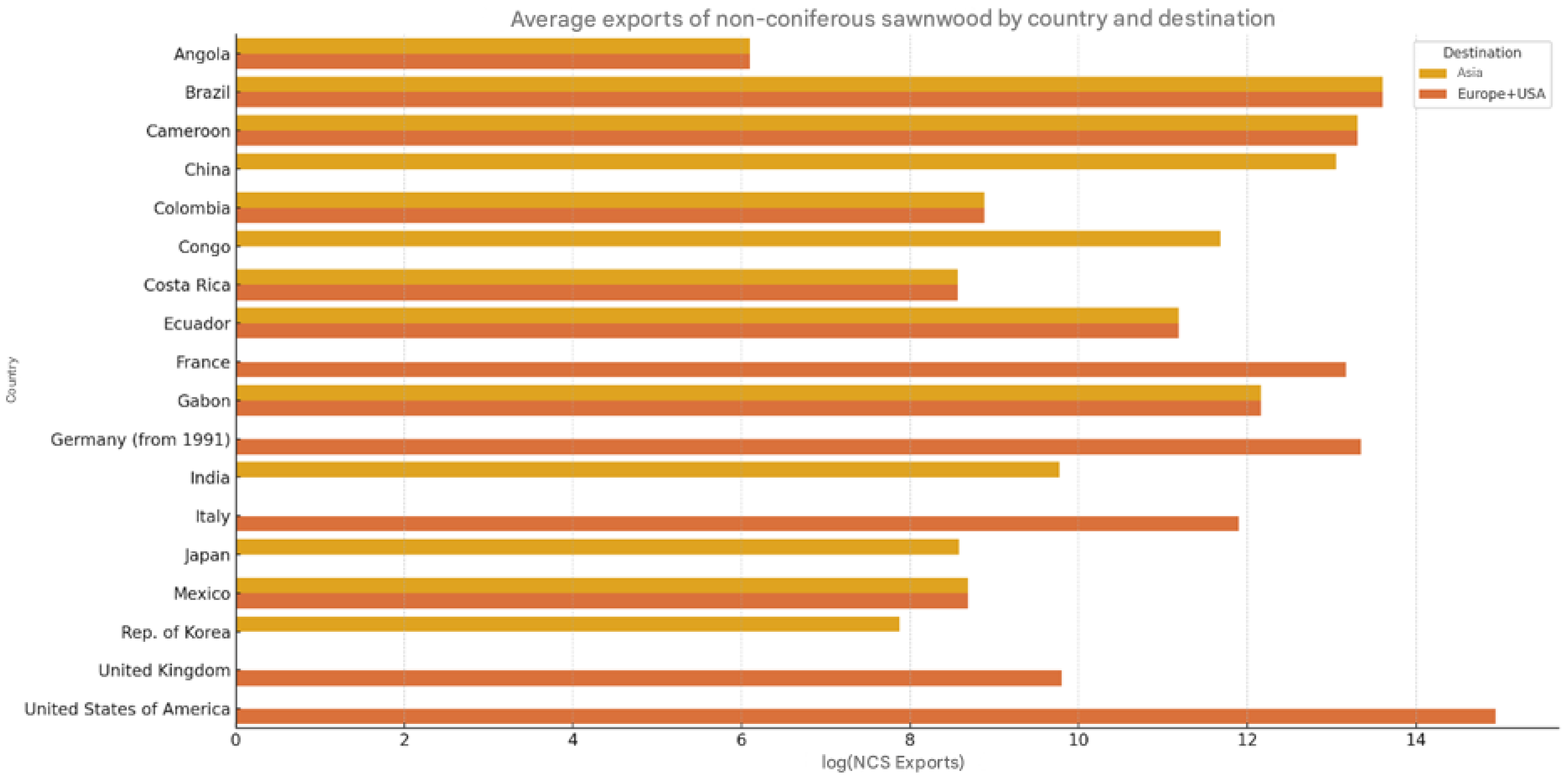
Some African countries have significantly lower export levels than their American counterparts. Asia appears to be a dominant destination for some countries, while others remain mainly focused on Europe or the United States.

4.3.1.2. Environmental Issues: An Asymmetrical Ecological Burden

The tropical forests of Central Africa, particularly those of the Congo Basin, are under intense and increasing ecological pressure, illustrated by an annual deforestation rate estimated at 0.18%, representing a loss of around 1.1 million hectares per year (GFW, 2023). Yet these ecosystems are essential to global climate balance, playing a crucial role by storing nearly 2.5 gigatons of CO₂ per year and being home to over 10,000 endemic species (Nepstad et al., 2022). Despite their importance, international tropical timber trade flows reproduce glaring environmental asymmetries. Indeed, only 12% of African sawnwood is certified to FSC or PEFC standards, compared with 35% in Europe [34], reflecting unequal access to sustainable standards. What's more, the absence of mirror clauses in trade agreements enables importing countries in the North to avoid applying to imported products the environmental standards they demand of their own producers [42]. In geopolitical terms, this asymmetry is accompanied by a high concentration of market power, particularly in favor of China, which holds over 60% of forest concessions in Central Africa [43]. This dominant position enables it to exert pressure on prices, having led to a 20% drop in export margins between 2015 and 2022 (ITTO, 2023). Furthermore, forest governance remains deficient: up to 30% of Cameroon's exported sawnwood comes from illegal logging [45], while producing countries have an average corruption index of just 28 out of 100, undermining transparency in the awarding of concessions (Transparency International, 2023).

4.4. Towards a Fair and Digital Tropical Timber Trade Model: Rebalancing Strategies and Sustainable Industrialization

The international trade in tropical hardwoods remains marked by profound structural inequalities inherited from colonial history and perpetuated by extractive specialization. This dynamic is reflected in low local processing, asymmetrical capture of added value by importing countries, persistent macroeconomic dependence and uncompensated ecological pressure. Econometric results from ARDL models and Granger causality tests confirm this subaltern trajectory in the international division of labor. In the face of these imbalances, a multidimensional strategy is proposed for achieving fairer, more sustainable trade, built around local processing, the valorization of environmental services, and technological governance.

The first approach is to rebalance value chains through targeted industrialization, notably by supporting Special Economic Zones (SEZ), as illustrated by the example of Gabon (GSEZ). Tax incentives, modulated according to the degree of processing of exported products, would help to promote industrial upgrading. In parallel, the internalization of ecological externalities involves the development of Payments for Environmental Services (PES) mechanisms and the adoption of blockchain-based traceability technologies (e.g. EUTR 2024). These innovations aim to guarantee the legal and ecological origin of wood flows.

On the geopolitical front, the creation of South-South alliances, such as a regional cartel between Gabon, Cameroon, DRC and Congo, is envisaged to strengthen the bargaining power of producer countries. The introduction of mirror clauses in trade would also make it possible to establish normative symmetry in social and environmental matters. Civil society and local NGOs play a crucial role in this respect, ensuring forest transparency via independent observatories.

In this context, forestry SEZs represent a major strategic lever. Three structuring objectives have been set for the 2030-2040 timeframe: to increase the proportion of wood processed locally to over 50%, to increase industrial added value through the export of labor-intensive products (furniture, panels, veneers), and to integrate ecosystem services through REDD+ and PES schemes. The operational architecture of the SEZs is organized around four strategic axes: industrialization through forest clusters, financing through sovereign and green funds, standardization through mandatory certification (FSC, PEFC), and training through skills centers in partnership with the European Union and China. A differentiated tax system (export duties of 0% for finished products, 20% for sawn timber and 30% for logs) and trade advantages under the APV-FLEGT and Belt and Road Initiative support this dynamic.

Strengthening the negotiating power of producer countries also calls for the implementation of a new business model within the International Tropical Timber Organization (ITTO), with precise performance indicators: a local processing rate of over 50%, an environmental certification rate of at least 40%, and a 150% increase in revenues per m³ exported. Innovative multilateral governance, including a blockchain-based Tropical Timber Observatory and a specialized trade tribunal, complete this arsenal to combat dumping and under-invoicing practices.

The expected impacts of this SEZ strategy are multidimensional: on the economic front, a ten-fold increase in employment thanks to local processing; on the ecological front, more sustainable exploitation of primary forests; on the geopolitical front, greater bargaining power for producer countries.

At the same time, the transition to a digitized, intelligent timber industry is a fundamental pillar of modernization. Artificial intelligence (AI) and digital technologies offer concrete solutions to strengthen traceability (blockchain certification, drone and satellite surveillance), add value to ecological services (carbon markets, bioacoustics), automate industrial transformation (smart factories, direct sales platforms), and increase commercial governance (ITTO 2.0, smart contracts, DAO). These innovations are aimed at reducing illegal timber by 40%, doubling local processing, increasing carbon revenues by 30% and reducing the corruption index in the industry by 20%.

Implementation relies on a synergy between public players, multilateral institutions (ITTO, FAO), technology startups (e.g. Satelligence) and green investors (e.g. CAFI). In the short term, the launch of blockchain pilot projects in Gabon and Cameroon, and the creation of a green forest innovation fund, could catalyze this transformation.

In short, this strategy proposes a structural overhaul of the tropical timber trade based on economic justice, environmental sustainability and technological innovation. It offers a credible response to global asymmetries, and paves the way for greater economic sovereignty for forest countries.

5. Discussion

The results of this study highlight the complexity of the dynamics underlying international trade in tropical hardwood sawnwood, revealing lasting structural imbalances between producer countries in the South and importer countries in the North. Econometric analysis using the CS_ARDL_CCE model, combined with Granger causality tests, confirms significant structural links between tropical wood exports and several explanatory variables. In particular, the positive effect of local production (logP_SNC) on exports in the long term (coefficient of 0.38) suggests that the strengthening of productive capacities remains a driving factor in forestry trade, corroborating the observations of Barbier and Burgess (2001). However, the lack of a short-term response is in line with the findings of Amacher et al. (2009), who highlight the inertia of supply chains. On the other hand, the positive and significant correlation of imports (logISNC) in both the short term (0.33) and long term (0.37) supports the hypothesis of increasing vertical integration in supply chains, similar to Asian models where log imports fuel local processing before re-export [49,50]. The robust effect of population (logPOP_T) in the long term (1.29) testifies to the importance of scale effects and sector specialization dynamics induced by population density, in line with endogenous growth models [51,52] and the work of López et al. (2007). On the other hand, the relatively low impact of economic growth (GDP_g) indicates a lower sensitivity of forestry exports to general macroeconomic variables, as also noted by Bohn and Deacon (2000) in resource-rich contexts. The results of the Granger tests shed further light: the bidirectional causality between exports and imports validates the idea of increased interdependence between industry segments [36,60], while the unidirectional relationship between population and exports confirms the catalytic effect of domestic demand, in line with the theories of Balassa (1985) and the work of [55].

However, these trade dynamics take place against a backdrop of strong structural inequalities and unbalanced capture of added value. African countries remain confined to exporting raw materials that are little or unprocessed, with a processing rate of less than 20%, while industrialized countries appropriate the rents arising from processing (Karsenty, 2016; Putzel et al., 2014). This situation stems from several interrelated constraints: insufficient industrial infrastructure, energy and skilled human resources hamper upmarketing (Weng et al., 2014; Hansen et al., 2018); the global tariff structure still puts exports of finished products at a disadvantage [56]; and the dominance of foreign players in forest concessions limits local spin-offs (Oyono et al., 2012; Colfer & Capistrano, 2005). These elements are part of a typical "resource curse" configuration (Sachs & Warner, 1999), reinforced here by often deficient forest governance (Andersen et al., 2012).

At the same time, environmental issues raise major concerns about the sustainability of the current model. The Congo Basin suffers an annual deforestation rate of 0.18%, while trade flow traceability mechanisms remain embryonic (GFW, 2023). Less than 12% of African exports are certified to FSC or PEFC standards, compared with over 35% in Europe [34], a gap amplified by the absence of mirror clauses that would unify requirements between domestic and imported production (Ekins et al., 2019; [59]. These deficits are part of an institutional context weakened by corruption, weak administrative capacity and recurrent failure to enforce regulations (Espach, 2009; [57,58].

Given these facts, forestry policies need to be reoriented towards a more equitable and sustainable model. Three main strategic avenues have emerged. Firstly, industrialization via special economic zones (SEZs) represents a promising lever for increased local processing. The case of the Nkok GSEZ in Gabon is a successful illustration of this, thanks to a coherent articulation between tax incentives, integrated logistics and public-private partnerships (Atanda, 2022; [1]. Recourse to climate financing such as REDD+ or the Green Climate Fund would align environmental imperatives with industrial objectives (Angelsen et al., 2012; Seymour & Harris, 2019). Secondly, better geopolitical coordination, notably via the International Tropical Timber Organization (ITTO), could enable producer countries to strengthen their bargaining power. The hypothesis of a cartel inspired by OPEC (Gilbert, 1989; Garsous, 2019) would aim to stabilize prices while reducing deleterious competition. The use of traceability technologies such as blockchain, already explored as part of the EUTR regulation (EU, 2013; del Gatto, 2021), could enhance transparency and limit illegal flows. Finally, the internalization of ecosystem services, through payments for environmental services (PES), needs to be expanded and better targeted, notably through schemes such as the CAFI program in Central Africa [9,61]. Supporting voluntary certification for SMEs would be a way of opening up access to premium markets while disseminating sustainability standards (Cashore et al., 2006; Espach, 2009).

There are, however, certain limitations to this research. Despite the richness of the panel used, several institutional variables such as transparency, political stability or corruption could not be included, which could affect the accuracy of the results. In addition, the heterogeneity of national trade policies is a source of unobserved bias. Future research would benefit from mobilizing finer environmental indicators (carbon footprint, ecological connectivity) and analyzing the intra-national distribution of value added in forest value chains (Duruflé et al., 2013; Gereffi, 2014). Ultimately, the results obtained call for a structural transformation of tropical forestry policies, based on upmarket exports, better regional coordination, and enhanced international recognition of ecosystem services. The development of South-South cooperation, green industrialization and reform of trade governance are the pillars of a more equitable, sustainable and resilient model.

6. Policy Implications and Recommendations

The empirical findings of this study highlight several strategic policy levers that can help reorient international trade in tropical hardwood lumber toward greater equity, sustainability, and value addition for producing countries. The implications span key areas such as industrial development, trade regulation, forest governance, regional integration, and ecosystem service valorization.

First, the positive and significant relationship between domestic production and export performance supports the case for accelerating local value addition. Strengthening domestic wood processing industries can reduce overreliance on raw log exports and enhance economic diversification. To this end, policy measures should prioritize the implementation of incentive-driven industrial strategies, including targeted tax exemptions, improved energy access, and dedicated investment support for processing activities such as drying, planing, and assembly. Moreover, the development of integrated and environmentally conscious Special Economic Zones (SEZs)—as exemplified by the Gabon Special Economic Zone (GSEZ)—should be promoted, ensuring alignment with national climate goals and social development priorities (Toman & Jemelkova, 2003; UNCTAD, 2021).

Second, reinforcing forest governance and improving traceability mechanisms are critical for combating illegal logging and ensuring sustainable trade. The persistent institutional weaknesses and loopholes in certification systems undermine regulatory effectiveness. Strengthening national forestry administrations, digitizing logging permits, and enhancing human resource capacity through training programs are essential steps. Additionally, the adoption of digital traceability technologies—particularly blockchain—can improve transparency across supply chains, drawing lessons from pilot initiatives in countries such as Ghana and Brazil (FAO, 2020; World Bank, 2022). Support for the wider adoption of sustainability certifications (e.g., FSC, PEFC, TLAS) through subsidies or technical assistance for small and medium enterprises (SMEs) is also recommended.

Third, international trade governance must be reformed to eliminate structural disadvantages faced by tropical timber-exporting countries. The continued dominance of raw material exports is partly explained by tariff escalation and the absence of equitable environmental clauses in trade agreements. In response, reforms to the World Trade Organization (WTO) framework should be pursued, including the removal of tariff barriers on processed wood products and the introduction of environmental mirror clauses for tropical timber imports (Howse & Eliason, 2005). Furthermore, producer countries should be encouraged to establish a coordination mechanism akin to a forestry consortium or cartel to harmonize export policies, stabilize prices, and increase their bargaining power vis-à-vis major importing blocs (e.g., EU, China).

Fourth, enhancing regional integration and fostering South-South cooperation can help overcome the limitations of fragmented national markets. Promoting intra-regional trade in processed timber through preferential trade agreements within regional blocs such as ECOWAS, ECCAS, or ASEAN would be beneficial. Additionally, establishing regional processing hubs with shared infrastructure—such as transportation networks, energy systems, and port facilities—could enhance economies of scale and competitiveness, especially in high-potential trade corridors (UNECA, 2020).

Finally, it is essential to integrate the valuation of ecosystem services provided by tropical forests—such as carbon sequestration and biodiversity conservation—into trade policy frameworks. Strengthening Payment for Environmental Services (PES) schemes, particularly those involving artisanal producers and local communities, can be achieved through mechanisms like REDD+, CAFI, or the Green Climate Fund (GCF). Developing eco-labeling systems tailored to tropical timber products, which combine environmental performance, social inclusion, and traceability, is another promising avenue. Importantly, international buyers should be required to commit to verifiable environmental standards as part of bilateral trade arrangements, such as Voluntary Partnership Agreements (VPAs) under the EU FLEGT Action Plan (European Commission, 2018).

Overall, these policy recommendations call for a multi-level, cross-sectoral approach that integrates industrial policy, trade regulation, environmental governance, and international cooperation. Only a coordinated and politically committed strategy—backed by strong international support—can reposition the tropical hardwood lumber trade as a vector for sustainable development in the Global South.

7. Conclusion

The dynamic and static analysis of international trade in tropical hardwood sawnwoods has highlighted the existence of persistent structural inequalities, revealing a trade model that does little to encourage the creation of added value in producing countries. Empirical results confirm that domestic forest production is a decisive lever for exports, while variables such as demographic size or per capita income have only a marginal effect. This finding underlines the need to move beyond a logic of primary specialization inherited from colonial history and reproduced by current world trade structures.

Beyond the diagnosis, this study proposes concrete avenues for reform based on better regional integration, stronger local processing, reinforced forest governance and explicit valuation of ecosystem services. It also calls for a redefinition of North-South trade relations to make them fairer, more sustainable and more transparent. The transition to an inclusive, circular, low-carbon forestry economy in tropical countries is not just an environmental necessity: it also represents a strategic opportunity to regain industrial and commercial sovereignty over resources that have long been undervalued.

Finally, this work paves the way for future in-depth studies. The introduction of environmental variables (deforestation rates, CO₂ emissions linked to logging), the analysis of value chains or even the study of the role of public policies in structuring trade flows would deserve to be investigated in future work. For it is in a better understanding of the structural, economic and ecological dynamics of the tropical timber trade that the key to truly sustainable forestry development lies.

References

- ITTO. Tropical Timber Market Report; International Tropical Timber Organization: Yokohama, Japan, 2023. [Google Scholar]
- Lebedys, A.; Li, Y. Contribution of the Forestry Sector to National Economies, 1990–2011; FAO: Rome, Italy, 2014. [Google Scholar]
- Piketty, T. Capital in the Twenty-First Century; Harvard University Press: Cambridge, MA, USA, 2015. [Google Scholar]
- Hansen, C.P.; Treue, T. Assessing illegal logging in Ghana. Int. For. Rev. 2008, 10, 573–590. [Google Scholar] [CrossRef]
- Cerutti, P.O.; Assembe-Mvondo, S.; German, L.; Putzel, L. The domestic market for small-scale chainsaw milling in Ghana. Int. For. Rev. 2011, 13, 167–179. [Google Scholar]
- Karsenty, A. Overview of Industrial Forest Concessions and Concession-Based Industry in Central and West Africa; World Bank: Washington, DC, USA, 2007. [Google Scholar]
- Tieguhong, J.C.; Ingram, V.; Schure, J.; Ewane, M.; Fomété, T. The impacts of artisanal logging on the livelihoods of forestry communities. Int. For. Rev. 2010, 12, 180–191. [Google Scholar]
- Barbier, E.B.; Burgess, J.C.; Grainger, A. Explaining agricultural land expansion and deforestation in developing countries. Am. J. Agric. Econ. 2005, 87, 1347–1353. [Google Scholar] [CrossRef]
- FAO. The State of the World's Forests; FAO: Rome, Italy, 2020. [Google Scholar]
- Roda, J.M.; Cuny, P.; Nasi, R. Atlas of tropical woods; CIRAD: Montpellier, France, 2016. [Google Scholar]
- Eba’a Atyi, R.; Lescuyer, G.; Ngouhouo Poufoun, J.; Moulendè Fouda, T. The Forests of the Congo Basin: State of the Forest 2013; CIFOR: Bogor, Indonesia, 2013. [Google Scholar]
- Gonçalves, M.P.; Panjer, M.; Greenberg, T.S.; Magrath, W.B. Charcoal-related Forest degradation dynamics in dry African woodlands. Environ. Res. Lett. 2012, 7, 045012. [Google Scholar]
- Humphreys, D.; Clegg, P.; Johnson, R. Forests: The shadow of civilization. In Environmental Issues in Political Discourse; Palgrave Macmillan: London, UK, 2006; pp. 123–145. [Google Scholar]
- Asner, G.P.; Rudel, T.K.; Aide, T.M.; Defries, R.; Emerson, R. A contemporary assessment of change in humid tropical forests. Conserv. Biol. 2009, 23, 1386–1395. [Google Scholar] [CrossRef] [PubMed]
- Karsenty, A. Large-scale acquisition of rights on forest lands in Africa. Int. For. Rev. 2010, 12, 1–8. [Google Scholar]
- Cerutti, P.O.; Tacconi, L.; Lescuyer, G.; Nasi, R. Legal vs. certified timber: Preliminary impacts of forest certification in Cameroon. For. Policy Econ. 2014, 48, 47–55. [Google Scholar] [CrossRef]
- Global Witness. Total Systems Failure: Exposing the Global Secrecy Destroying Forests; Global Witness: London, UK, 2019. [Google Scholar]
- Auty, R.M. Resource Abundance and Economic Development; Oxford University Press: Oxford, UK, 2001. [Google Scholar]
- Köhlin, G.; Sills, E.O.; Pattanayak, S.K.; Wilfong, C. Energy, gender and development: What are the linkages? World Bank Policy Research Working Paper No. 5800, 2011. [Google Scholar]
- Venables, A.J. Using natural resources for development: Why has it proven so difficult? J. Econ. Perspect. 2016, 30, 161–184. [Google Scholar] [CrossRef]
- Gylfason, T. Natural resources, education, and economic development. Eur. Econ. Rev. 2001, 45, 847–859. [Google Scholar] [CrossRef]
- Bertrand, A. Wood in Africa; Karthala: Paris, France, 1978. [Google Scholar]
- Lesniewska, F.; McDermott, C. FLEGT VPAs: Laying a pathway to sustainability via legality lessons from Ghana and Indonesia. For. Policy Econ. 2014, 48, 16–23. [Google Scholar] [CrossRef]
- Ezzine-de-Blas, D.; Mas, J.F.; del Mar López, M.; Nilsson, M.; Wunder, S. Forest loss and livelihoods in tropical forests: Panel data evidence from Madagascar. World Dev. 2011, 39, 808–816. [Google Scholar]
- Angelsen, A.; Larsen, H.O.; Lund, J.F.; Smith-Hall, C.; Wunder, S. Environmental income and rural livelihoods: A global-comparative analysis. World Dev. 2014, 64, S12–S28. [Google Scholar] [CrossRef]
- Kaplinsky, R.; Morris, M. A Handbook for Value Chain Research; IDRC: Ottawa, ON, Canada, 2001. [Google Scholar]
- Karsenty, A.; Ongolo, S. Can "fragile states" decide to reduce their deforestation? For. Policy Econ. 2012, 18, 38–45. [Google Scholar] [CrossRef]
- Oyono, P.R.; Biyong, M.B.; Samba, S.V. Beyond the extraction: The social and ecological impacts of industrial logging in Central Africa. Environ. Manag. 2015, 55, 227–240. [Google Scholar]
- Buttoud, G. Les politiques forestières en Afrique francophone; L’Harmattan: Paris, France, 1995. [Google Scholar]
- Sales, A. Le commerce international des bois tropicaux; Economica: Paris, France, 1999. [Google Scholar]
- De Jong, W.; Galloway, G.; Katila, P.; Pacheco, P.; Pokorny, B. Forest and Land-Use Governance in a Decentralized World; Routledge: London, UK, 2017. [Google Scholar]
- Tacconi, L. Illegal Logging: Law Enforcement, Livelihoods and the Timber Trade; Earthscan: London, UK, 2007. [Google Scholar]
- Cashore, B. Global Forest Governance; Cambridge University Press: Cambridge, UK, 2023. [Google Scholar]
- Cerutti, P.O.; Lescuyer, G.; Tsanga, R.; Mendoula, E.E.; Medjibe, V. Forest certification in Central Africa: Recent advances and persistent challenges. For. Policy Econ. 2021, 45, 102–113. [Google Scholar]
- FAO. State of the World's Forests 2022; FAO: Rome, Italy, 2022. [Google Scholar]
- Sun, L.; Canby, K. China’s Forest Trade; Rights and Resources Initiative (RRI): Washington, DC, USA, 2021. [Google Scholar]
- Prebisch, R. The Economic Development of Latin America and Its Principal Problems; United Nations: New York, NY, USA, 1950. [Google Scholar]
- Angelsen, A.; Rudel, T.K. Tropical Deforestation: Causes and Consequences; Cambridge University Press: Cambridge, UK, 2022. [Google Scholar]
- Hurmekoski, E.; Lovrić, M.; Hetemäki, L. Transnational value chains in the forest sector. For. Policy Econ. 2022, 136, 102623. [Google Scholar]
- Pendrill, F.; Persson, U.M.; Godar, J.; Kastner, T. The impact of global trade on deforestation. Environ. Sci. Policy 2023, 130, 35–43. [Google Scholar]
- Geist, H.J.; Lambin, E.F. Proximate causes and underlying driving forces of tropical deforestation. BioScience 2002, 52, 143–150. [Google Scholar] [CrossRef]
- Meyfroidt, P. Global land use change, economic globalization, and the looming land scarcity. Proc. Natl. Acad. Sci. USA 2011, 108, 3465–3472. [Google Scholar]
- Zhang, Y. Forest Concession Politics in Central Africa; CIFOR: Bogor, Indonesia, 2023. [Google Scholar]
- WWF. Timber Transformation and Value Chains; WWF: Gland, Switzerland, 2023. [Google Scholar]
- Global Witness. Exporting Destruction; Global Witness: London, UK, 2022. [Google Scholar]
- World Bank. Creating Markets in Forest-Rich Countries; World Bank: Washington, DC, USA, 2022. [Google Scholar]
- Barbier, E.B.; Burgess, J.C. The economics of tropical deforestation. J. Econ. Surv. 2001, 15, 413–433. [Google Scholar] [CrossRef]
- Amacher, G.S.; Ollikainen, M.; Koskela, E. Economics of Forest Resources; MIT Press: Cambridge, MA, USA, 2009. [Google Scholar]
- Ribot, J.C. Choice, recognition and the democracy effects of decentralization. IDS Bull. 2005, 36, 43–50. [Google Scholar]
- Wertz-Kanounnikoff, S.; Angelsen, A. Global and national REDD+ architecture: Linking institutions and actions. In Analysing REDD: Challenges and Choices; CIFOR: Bogor, Indonesia, 2009; pp. 13–24. [Google Scholar]
- Romer, P. Endogenous technological change. J. Polit. Econ. 1990, 98, S71–S102. [Google Scholar] [CrossRef]
- Aghion, P.; Howitt, P. Endogenous Growth Theory; MIT Press: Cambridge, MA, USA, 1998. [Google Scholar]
- López, R.; Thomas, V.; Wang, Y. The Economics of Natural Resources in Latin America; World Bank: Washington, DC, USA, 2007. [Google Scholar]
- Bohn, H.; Deacon, R.T. Ownership risk, investment, and the use of natural resources. Am. Econ. Rev. 2000, 90, 526–549. [Google Scholar] [CrossRef]
- Hausmann, R.; Hwang, J.; Rodrik, D. What you export matters. J. Econ. Growth 2007, 12, 1–25. [Google Scholar] [CrossRef]
- Hoekman, B.M.; Kostecki, M.M. The Political Economy of the World Trading System; Oxford University Press: Oxford, UK, 2009. [Google Scholar]
- Kaimowitz, D. Forests and governance: A review of the key issues. CIFOR Occas. Pap. 2003, 32, 1–36. [Google Scholar]
- Larson, A.M.; Ribot, J.C. The poverty of forestry policy: Double standards on an uneven playing field. World Dev. 2007, 35, 1945–1961. [Google Scholar] [CrossRef]
- Ponte, S. Green trade and private governance. Rev. Int. Political Econ. 2022, 29, 189–215. [Google Scholar]
- Simula, M. Analysis of incentives and value chains for sustainable forest management. ITTO Tech. Ser. 2010, 34, 1–85. [Google Scholar]
- Wunder, S. The efficiency of payments for environmental services in tropical conservation. Conserv. Biol. 2007, 21, 48–58. [Google Scholar] [CrossRef] [PubMed]