
Submitted:
19 June 2025
Posted:
20 June 2025
You are already at the latest version
Abstract
This work examines a system of n singularly perturbed robin-type initial value problems with discontinuous source terms. Each equation’s derivative component is multiplied by the same singular perturbation parameter (ε). A piecewise uniform Shishkin mesh is built and used, together with a classical finite difference scheme, to create a numerical technique for addressing the problem. It is demonstrated that the numerical approximations produced by this method are effectively first order convergent in the maximum norm at all places in the domain, uniformly with regard to the singular perturbation parameter. Numerical findings are offered to support the theory.
Keywords:
singular perturbation problems
; mixed-type initial conditions
; finite difference methods
; discontinuous source terms
; Shishkin-type meshes
; uniform convergence with respect to the perturbation parameter
1. Introduction
Singularly perturbed initial–boundary value problems occur frequently across applied mathematics and engineering disciplines. For example, systems of first-order, singularly perturbed ordinary differential equations are fundamental in chemical reactor modeling. The small magnitude of the perturbation parameters induces a multi-scale behavior that typically precludes closed-form solutions. Consequently, the exact solution often features sharply varying layers—initial, boundary, or interior—confined to narrow regions. Over the past several decades, a variety of numerical schemes that achieve uniform convergence with respect to these small parameters have been developed and analyzed.
Examine a Robin-type, singularly perturbed initial-value system with discontinuous sources over , assume the source term is discontinuous at a single point d within the domain . Let and . The jump of a function at the point d is defined by
where and denote the right and left limits of at d, respectively. The problem can be stated as finding the solution to the initial value problem , such that
along with the initial conditions provided
where, and .
From (1) and (2), the problem can equivalently be expressed in operator form as follows:
with
where the definitions of the operators are given by
Here, the operator I is the identity, and signifies the first derivative operator.
Assumption 1.
The functions satisfy the following positivity conditions
Assumption 2.
The positive value α adheres to the inequality
Assumption 3.
The parameter ε, representing the singular perturbation and distinct, is assumed to satisfy .
The given problem is singularly perturbed in the sense that setting in system (1) yields the following reduced linear algebraic system.
where and .
The source terms are sufficiently smooth throughout except at the point d. The component of the solution of problem (1) and (2) display initial layers that overlap at and interior layers that overlap just to the right of the discontinuity located at
For a detailed account of parameter-uniform numerical techniques used in the study of singular perturbation problems, see [3,4,6]. The seminal work of Shishkin [8] laid the groundwork for addressing singularly perturbed reaction-diffusion equations with discontinuous coefficients. In the context of scalar equations, Dunne and Riordan [2] investigated initial value problems exhibiting singular perturbations and discontinuous data. Numerical methods that maintain robustness with respect to the perturbation parameter for systems of such problems were discussed in [7]. In [12] a parameter-uniform numerical method was developed for systems where all singular perturbation parameters are equal, leading to solution components with initial layers of uniform width and thus simplifying the analysis. The case in which the singular perturbation parameter appears in only one of the equations was examined in [5]. The most general and challenging scenario, involving individual initial layers for each solution component that overlap and influence one another, has been studied in [1,9,13]. Notably, [9] introduced a uniformly convergent numerical method of first order accuracy (up to a logarithmic factor), while [1] proposed a hybrid finite difference scheme on a piecewise-uniform Shishkin mesh achieving nearly second-order accuracy uniformly with respect to both small parameters. In all these previous studies, the source term was assumed to be smooth. In contrast, the present work deals with discontinuous source terms, resulting in each solution component exhibiting both initial and interior layers.
Proof.
Examine and as the specific solutions to the differential equations
and
Let us analyze the function
where is the solution of
Here is chosen so that . In The function cannot attain an internal maximum or minimum, and therefore, in . Choose the constants such that
The existence of the constants requires that
Since , the existence of and consequently is guaranteed. □
Remark: In this section, C stands for a general vector of positive constants, which remain unaffected by the perturbation parameters and the discretization parameter N.
2. Mathematical Analysis
The operator adheres to the following maximum principle.
Lemma 1.
Proof.
Assume that meets the requirements specified in (5) and (6). Let be a function such that
and
Then it follows that
Case (i):
and
Case (ii):
Given that and , there exists a neighborhood around d where holds for every . Select a point , distinct from d, such that . By the Mean Value Theorem, there exists some for which
Since lies within , an argument analogous to that used in the first case implies that,
thus arriving at a contradiction. □
As a straightforward implication of the previous lemma, the following stability result holds.
Proof.
Introduce the pair of functions
where . Then, it is true that , by a proper choice of C and on . It follows from Lemma 1 that on Hence,
□
Lemma 3.
Proof.
The argument proceeds analogously to the proof of Lemma 2 in [11].
3. Estimates for the Derivative Components
To obtain more precise derivative estimates, we split the solution into a regular part and a singular part , such that
The regular component is defined to satisfy the following boundary value problem:
Correspondingly, the singular component is defined as the solution to the problem described below:
□
Proof. The findings can be established by utilizing the techniques described in [9].
Also for ,
and
Similarly, , and hence the proof is completed. □
We now aim to find bounds on the layer components of . Consider the layer functions:
Proof. Since , and by Lemma 2 we have and , we proceed by introducing the barrier function
where C is chosen sufficiently large so that at and .
It is straightforward to verify that . Applying the maximum principle (1), we obtain the desired bounds on . To bound the first-order derivative of , consider the equation
along with the established bounds on . This implies that
To obtain a sharper bound, consider the system of equations
To derive a more accurate bound, we analyze the reduced system consisting of equations:
where and are the matrices obtained by eliminating the last row and column of E and A, respectively. The vector has components defined by for . By utilizing previously derived bounds and decomposing into its regular and singular components, , we can establish the required result.
To estimate the second derivatives, we differentiate the equation
once more. Applying earlier bounds on then yields the desired estimates for the singular component and its derivatives. □
A finer decomposition of the singular component is required to facilitate the convergence analysis. The next Lemma provides the necessary estimates of decomposed layer functions.
Theorem 4.
For each , the singular component can be broken down as follows:
where
Proof. Define a function as follows
and for , we have
We now determine the estimates for the second derivative.
For .
For .
Now for each , from this, it can be inferred that
On the interval ,
On the interval .
On the interval ,
On the interval .
The relation corresponding to the bounds of the first derivatives is given by:
□
4. The Shishkin-Type Mesh
Consider a piecewise-uniform Shishkin mesh consisting of N mesh intervals, constructed in the following manner. The domain is partitioned into four subintervals:
A uniform mesh with points is then generated on each of these subintervals. The interior mesh points are denoted by .
Clearly, the midpoint of the mesh satisfies , and the mesh is given by . Note that the mesh reduces to a uniform mesh when and . To adapt the mesh for the singularly perturbed problem (1), the parameters and are selected as functions depending on N and .
5. Formulation of the Discrete Problem
Problems (1) and (2), which are of mixed initial value type, are numerically solved using a fitted mesh framework based on the piecewise-uniform grid and standard finite differences. The resulting scheme for takes the form:
with
and at , the numerical scheme is formulated as
The system described by (13) and (14) can be cast into operator form as well.
The operators and represent forward and backward difference operators, respectively.
The subsequent discrete results exhibit behavior similar to that observed in the continuous setting.
Proof. Let be the point at which attains its minimum over . If , the result is immediate. Without loss of generality, assume that . In this case, it is evident that, . Indeed, if
Therefore, . If , it is apparent that
and hence if , then
which is a contradiction. It can therefore be inferred that . Then
From the above it is observed that
then, , this contradicts our assumption, completing the proof. □
Proof. We now introduce two mesh functions defined as follows
By leveraging the properties of , it can be readily shown that
Applying the discrete maximum principle (Lemma 4), it follows that
Consequently,
thereby establishing the result. □
6. Analysis of the Local Truncation Error
From Lemma 5, we observe that to estimate the error , it is sufficient to bound the quantity . Note that, for ,
and
This represents the local truncation error associated with the first derivative. By subsequently employing the triangle inequality,
The discrete solution is similarly decomposed into components and , eas in the continuous case.
and
where is the solution of (11) and is the solution of (12).
Furthermore, for every
The error at each mesh point is given by . Correspondingly, the local truncation error can be decomposed as follows:
Taylor series applied to both components—singular and regular—provides
and
where
The next section is dedicated to establishing error estimates for both the smooth and singular components.
7. Estimation of Numerical Errors
The validation of the error estimation theorem occurs in two stages: beginning with the evaluation of the smooth component error and then analyzing the singular component error.
Proof. The expression implies that (19),
It is straightforward to show that
thus satisfying the requirement. □
Proof. To show this Theorem, the accuracy estimates for singular components must be assessed at different sub intervals in the following manner:
Case (i): The solution strategy hinges on whether the transition parameter, is or .
Sub-case (i): When , the mesh is uniform and meets the condition .
The expression implies that (20),
The solution approach outlined above thus produces
Since , the estimate for obtained which gives
Therefore,
Sub-case (ii): For , the mesh is piecewise uniform, featuring a mesh size of on the interval and on the interval .
Case (ii): The solution strategy varies depending on whether the transition parameter equals or .
Sub-case (i): When , the mesh is uniform and satisfies the inequality .
Accordingly, by following the same arguments used in the initial case, the proof is concluded.
Sub-case (ii): For , the mesh becomes piecewise uniform with mesh widths on the segment and on .
From this, we deduce that
Focusing now on
□
By applying the discrete maximum principle and conducting error bound derivation for both the regular and singular components, we arrive at the following key result, which is presented in this section.
Proof. This proof mirrors the argument used in Theorem 2 of [10]. □
8. Numerical Experiment
This section illustrates the numerical method described above with a practical example.
Example 1.
We focus on the singularly perturbed mixed-type initial value problems characterized by discontinuous source terms, as given below.
with
where
As the exact solution for the test example is not known, the error in is estimated by comparing it with the numerical solution obtained on a finer mesh , which incorporates both the original mesh points and their midpoints. Calculations are carried out for different values of N and the perturbation parameter .
Figure 1 displays the numerical solution for Example 1 obtained through the fitted mesh method described by (13) and (14). The corresponding error constants and observed orders of convergence are summarized in Table 1.
9. Conclusions
In this paper, numerical methods are developed to solve linear systems of initial value problems characterized by identical singular perturbation parameters, discontinuous source terms, and Robin initial conditions. The proposed approach yields approximations that are uniformly convergent in the maximum norm across the perturbation parameter, with accuracy approaching first order. Numerical results, including convergence plots, confirm the first-order behavior of the schemes. Additionally, discrete derivatives of the solutions are computed and presented. The development of Shishkin meshes and corresponding numerical methods has proven to be both effective and intellectually engaging.
Author Contributions
Conceptualization, S.D.; methodology, S. D.; software, S.D.; validation, S.D., G.E.C., S.S and G.R.; formal analysis, S.D.; investigation, S.D., S.S.,G.R. and G.E.C.; resources, S.D.; data curation, S.D. and S.S.; writing—original draft preparation, S.D., S.S. and G.R.; writing—review and editing, S.D., S.S.,G.R. and G.E.C.; visualization, S.D.; supervision, G.E.C. and S.D.; project administration, S.D.; funding acquisition, G.E.C. All authors have read and agreed to the published version of the manuscript.
Funding
This research received no external funding.
Data Availability Statement
Data is contained within the article.
Conflicts of Interest
The authors declare no conflicts of interest.
References
- Cen, Z.; Xu, A.; Le, A. A second-order hybrid finite difference scheme for a system of singularly perturbed initial value problems. J. Comput. Appl. Math. 2010, 234, 3445–3457. [CrossRef]
- Dunne, R.K.; Riordan, E.O’. Interior layers arising in linear singularly perturbed differential equations with discontinuous coefficients. In: Proceedings of the Fourth International Conference on Finite Difference Methods: Theory and Applications. Lozenetz, Bulgaria 2006, 29–38.
- Doolan, E.P.; Miller, J.J.H.; Schilders, W. H. A. Uniform Numerical Methods for Problems with Initial and Boundary Layers, Boole Press, 1980.
- Farrell, F.A.; Hegarty, A.;Miller, J.J.H.; O’Riordan, E.; Shishkin, G. I. Robust computational techniques for boundary layers. In R.J. Knops, K.W. Morton (Eds.), Applied Mathematics & Mathematical Computation, Chapman & Hall/CRC Press, 2000.
- Maragatha Meenakshi, P.; Valarmathi, S.; Miller, J. J. H. Solving a partially singularly perturbed initial value problem on Shishkin meshes. Applied Mathematics and Computation 2010, 215, 3170–3180. [CrossRef]
- Miller, J.J.H.; O’Riordan, E.; Shishkin, G. I. Fitted numerical methods for singular perturbation problems. Error estimates in the maximum norm for linear problems in one and two dimensions. World Scientific publishing Co.Pvt.Ltd., Singapore 1996.
- Roos, H.G.; Stynes, M.; Tobiska, L. Robust numerical methods for singularly perturbed differential equations. Springer Series in Computational Mathematics, 2nd edn. Springer, Berlin 2008.
- Shishkin, G.I. Grid Approximations of Singularly Perturbed Elliptic and Parabolic Equations, Ural Branch of Russian Academy of Sciences 1992.
- Valarmathi, S.; Miller, J.J.H. A parameter-uniform finite difference method for singularly perturbed linear dynamical systems. Int. J. Numer. Anal. Model. 2010, 7, 535–548.
- Dinesh, S. Linear System of Singularly Perturbed Initial Value Problems with Robin Initial Conditions, Australian Journal of Mathematical Analysis and Applications 2023, 20(1), 1–16.
- Dinesh Selvaraj; Joseph Paramasivam Mathiyazhagan. A parameter uniform numerical method for a singularly perturbed initial value problem with Robin initial condition, Malaya Journal of Matematik 2020, 8(2), 414–420.
- Hemavathi, S.; Bhuvaneswari, T.; Valarmathi, S.; Miller, J.J.H. A parameter uniform numerical method for a system of singularly perturbed ordinary differential equations. Appl.Math. Comput. 2007, 191, 1–11. [CrossRef]
- Rao, S.C.S.; Kumar, S. Second order global uniformly convergent numerical method for a coupled system of singularly perturbed initial value problems. Appl.Math. Comput. 219, 3740–3753.
Figure 1.
The figure portrays the numerical solution associated with problem (1), calculated using . The solution components , , and display initial layers as well as a discontinuity located at .
Figure 1.
The figure portrays the numerical solution associated with problem (1), calculated using . The solution components , , and display initial layers as well as a discontinuity located at .
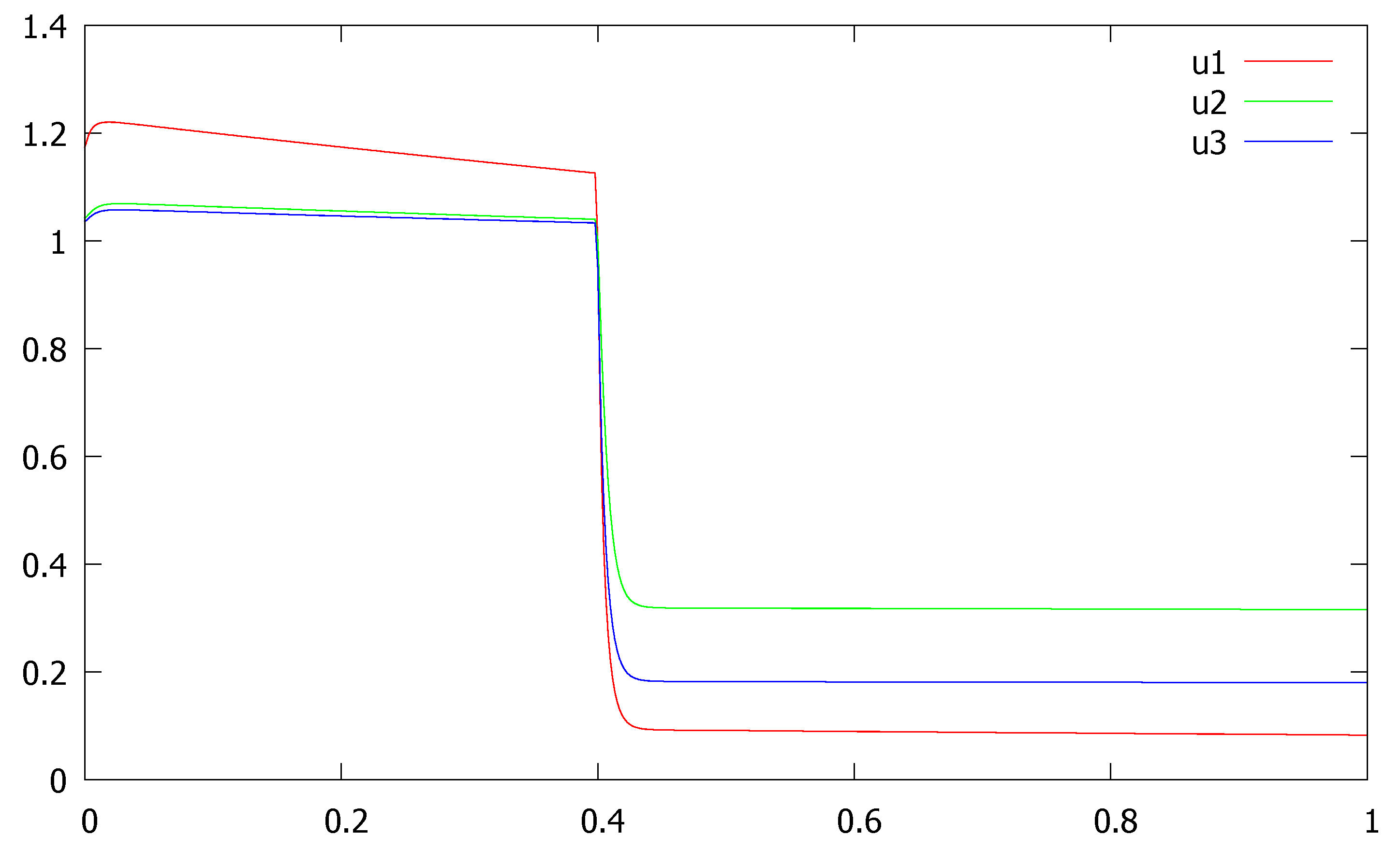

Table 1.
Maximum absolute errors at points and computed for the example.
| Number of discretization points | ||||
| 72 | 144 | 288 | 576 | |
| 0.100E+01 | 0.798E-02 | 0.436E-02 | 0.228E-02 | 0.117E-02 |
| 0.250E+00 | 0.171E-01 | 0.112E-01 | 0.655E-02 | 0.357E-02 |
| 0.625E-01 | 0.162E-01 | 0.129E-01 | 0.916E-02 | 0.597E-02 |
| 0.156E-01 | 0.160E-01 | 0.127E-01 | 0.903E-02 | 0.588E-02 |
| 0.391E-02 | 0.160E-01 | 0.126E-01 | 0.900E-02 | 0.586E-02 |
| 0.171E-01 | 0.129E-01 | 0.916E-02 | 0.597E-02 | |
| 0.409E+00 | 0.489E+00 | 0.618E+00 | ||
| 0.398E+00 | 0.398E+00 | 0.377E+00 | 0.326E+00 | |
| The order of -uniform convergence | ||||
| Computed -uniform error constant, | ||||
Disclaimer/Publisher’s Note: The statements, opinions and data contained in all publications are solely those of the individual author(s) and contributor(s) and not of MDPI and/or the editor(s). MDPI and/or the editor(s) disclaim responsibility for any injury to people or property resulting from any ideas, methods, instructions or products referred to in the content. |
© 2025 by the authors. Licensee MDPI, Basel, Switzerland. This article is an open access article distributed under the terms and conditions of the Creative Commons Attribution (CC BY) license (http://creativecommons.org/licenses/by/4.0/).
Copyright: This open access article is published under a Creative Commons CC BY 4.0 license, which permit the free download, distribution, and reuse, provided that the author and preprint are cited in any reuse.


