
Submitted:
19 June 2025
Posted:
20 June 2025
You are already at the latest version
Abstract
Geological hazards severely constrain urban construction planning and economic development, particularly for large and medium-sized cities. Xi'an City is located in the transitional zone between the Guanzhong Plain and the Qinling Mountains, characterized by complex geological conditions and frequent occurrence of various geological hazards, posing serious threats to regional economic development and the safety of residents' lives and property. Currently, diverse methods and models exist for geological hazard susceptibility assessment. Selecting appropriate evaluation models and assessment factors to conduct geological hazard susceptibility evaluation plays a crucial role in geological hazard risk management and economic development promotion in Xi'an City. Taking geological hazards throughout Xi'an City as the research object, this study analyzed the formation conditions and influencing factors of geological hazards. Via Spearman correlation analysis, appropriate evaluation indicators were selected, and a geological hazard susceptibility assessment system was constructed through the comprehensive application of the combined weighting method and information value model. The main research findings are as follows: (1) A total of 787 geological hazards (hidden danger points) have developed in Xi'an City, predominantly landslides (435 occurrences) and collapses (304 occurrences), distributed in loess landform areas and the Qinling mountainous region, while ground subsidence and ground fissures are mainly distributed in alluvial plain areas; (2) Twelve factors including slope gradient, slope aspect, and surface relief were selected as susceptibility evaluation indicators. The analytic hierarchy process was employed to determine subjective weights, the entropy weight method was used to calculate objective weights, and the distance function method was utilized to combine the two types of weights; (3) Four information value models were established: unweighted, subjective weighted, objective weighted, and combined weighted models. Through verification via hazard point density and ROC curves, the combined weighting information value model demonstrated the highest evaluation accuracy (AUC value of 0.872); (4) The combined weighting information value model was employed to assess geological hazard susceptibility in Xi'an City, resulting in classification into high susceptibility areas (1,305.36 km², accounting for 12.31%), moderate susceptibility areas (1,980.96 km², accounting for 18.68%), low susceptibility areas (835.48 km², accounting for 7.88%), and non-susceptible areas (6,485.72 km², accounting for 61.14%). The study demonstrates that the combined weighting method can overcome the limitations of single weighting approaches, and the evaluation results better conform to the distribution patterns of geological hazards in the study area, providing a scientific basis for geological hazard prevention and control in Xi'an City.
Keywords:
Xi'an City
; geological hazards
; susceptibility assessment
; combined weighting method
; information value model
1. Introduction
Geological hazards refer to disasters that endanger public life and property safety caused by natural factors or human activities, characterized by suddenness, persistence, and clustering, including landslides, collapses, debris flows, ground collapse, ground fissures, ground subsidence, and other disasters directly related to natural geological influences [1,2]. In recent years, with the acceleration of urbanization processes and the intensification of human engineering activities, the occurrence frequency of geological hazards and the resulting losses have demonstrated an upward trend, particularly in areas with complex geological conditions and dense populations, where geological hazards have become important factors threatening regional socioeconomic sustainable development [3,4]. As a significant city in Northwest China, Xi’an City is located in the transitional zone between the Guanzhong Plain and the Qinling Mountains, characterized by complex geological structures, complete stratigraphic development, significant topographic relief, pronounced seasonal rainfall patterns, and frequent human engineering activities. Various types of geological hazards occur frequently, seriously threatening the life and property safety of local residents and the healthy development of the city. Therefore, conducting geological hazard susceptibility assessment research in Xi’an City and scientifically delineating geological hazard-prone areas holds important theoretical and practical significance for guiding geological hazard prevention and control work and ensuring regional safety.
Geological hazard susceptibility assessment refers to the prediction and evaluation of the probability of geological hazard occurrence within specific regions, constituting an important component of geological hazard risk assessment [5,6]. Currently, geological hazard susceptibility assessment methods are primarily divided into two major categories: qualitative assessment and quantitative assessment. Qualitative assessment mainly includes expert experience methods, analytic hierarchy process, and fuzzy comprehensive evaluation methods, which, although simple to operate, are relatively subjective and yield evaluation results with relatively low accuracy and reliability [7,8]. With the development of 3S technology and computer technology, quantitative assessment methods have been widely applied, primarily encompassing mathematical statistical models and machine learning models [9,10]. Mathematical statistical models such as certainty factor models, information value models, and logistic regression models can objectively reflect the relationships between assessment factors and geological hazards, but face difficulties in handling complex nonlinear relationships [11,12]. In recent years, machine learning models such as random forest, support vector machine, XGBoost, and artificial neural networks have been widely applied in geological hazard susceptibility assessment due to their capability to process high-dimensional data and complex nonlinear relationships [13,14,15,16,17]. However, single models often possess limitations and cannot comprehensively reflect the complex causative mechanisms of geological hazards. Multi-model coupling and ensemble learning methods have attracted researchers’ attention because they can integrate the advantages of various models [18,19,20].
In the process of geological hazard susceptibility assessment, the determination of evaluation indicator weights constitutes a critical component that directly influences the accuracy of assessment results. Weight determination methods are primarily classified into three categories: subjective weighting methods, objective weighting methods, and combined weighting methods [21,22]. Subjective weighting methods, such as the analytic hierarchy process and Delphi method, rely on expert experience and subjective judgment, possessing clear physical significance, but often exhibit certain biases due to limitations of individual subjective cognition [23,24]. Objective weighting methods, such as the entropy weight method, coefficient of variation method, and principal component analysis, rely entirely on data information and can avoid interference from human factors, but may overlook the actual importance of indicators [25,26]. Combined weighting methods integrate the advantages of both subjective and objective weighting approaches, enabling more comprehensive and reasonable determination of evaluation indicator weights and enhancing the scientific validity and reliability of assessment results [27,28,29]. Wang Nianqin et al. [3] constructed a debris flow hazard susceptibility assessment cloud model based on the game theory combined weighting method, with evaluation results effectively reflecting the distribution patterns of debris flow hazards in the study area. Gao Xingxing et al. [29] achieved favorable results in evaluating geological hazard susceptibility in the Lüliang mountainous area based on statistical methods coupled with geographic detectors. Yu Xikun et al. [30] employed a coupled model of certainty factor and information value to conduct geological hazard susceptibility assessment in Emin County, Xinjiang, demonstrating the effectiveness of the combined weighting method.
As a region with frequent geological hazards, Xi’an City exhibits diverse geological hazard types, widespread distribution, and complex causative mechanisms, making traditional single weight determination methods inadequate for accurately reflecting the contribution of various influencing factors to geological hazard susceptibility. Based on the geological environmental conditions and geological hazard characteristics of Xi’an City, this study comprehensively analyzed the characteristics and development patterns of geological hazards in the study area to select appropriate evaluation indicators. Subsequently, the analytic hierarchy process was employed to determine subjective weights, the entropy weight method was used to calculate objective weights, and the linear weighting method was utilized to compute comprehensive weights. Finally, geological hazard susceptibility assessment was conducted based on the information value model, and the optimal assessment model was determined through comparative analysis, providing a scientific basis for geological hazard prevention and control planning in Xi’an City.
2. Study Area Overview
2.1. Physical Geography
Xi’an City is located in the south-central part of Shaanxi Province, between 107°40′–109°49′E longitude and 33°42′–34°45′N latitude. The city is bounded by the Bashanyuan Mountains to the east, extends to the Taibai Mountain area to the west, reaches the main ridge of the Qinling Mountains to the south, and borders the Wei River to the north. The city measures 204 km from east to west and 116 km from north to south, with a total area of 10,588.9 km2. The transportation network is well-developed, with the Xi’an Ring Expressway (G3002) serving as the hub where six national expressways converge, forming a “米”-shaped high-speed railway network comprising the Da(tong)-Xi(an) High-Speed Railway, Zheng(zhou)-Xi(an) High-Speed Railway, and others (Figure 1).
Xi’an City exhibits a warm temperate semi-humid continental monsoon climate, characterized by complex and variable regional topography and pronounced vertical climate distribution with outstanding regional differences. From north to south, with increasing elevation, temperature decreases while precipitation increases. The annual average precipitation is 599.42 mm, with a maximum of 903.2 mm (1983) and a minimum of 312.2 mm (1995). Precipitation is predominantly concentrated during July–September, accounting for approximately 49.23% of the annual rainfall. Xi’an City possesses abundant river development, primarily including the Wei River, Ba River, Chan River, Feng River, Hao River, Lao River, Hei River, and Jing River, among others, with the Wei River being the largest-scale river, flowing through the area for approximately 150 km.
2.2. Topography and Geomorphology
The study area exhibits complex and diverse topography and geomorphology, generally demonstrating a pattern of high elevation in the south and low elevation in the north, high elevation in the east and low elevation in the west. The main geomorphological types include: alluvial and alluvial-pluvial plain areas (accounting for approximately 30.11% of the total area), piedmont pluvial plain areas (approximately 8.25%), loess landform areas (approximately 12.08%), and mountainous regions (approximately 49.56%). The mountainous regions can be roughly divided into low mountain and hilly areas, middle mountain areas, and high mountain areas, with the middle mountain areas covering the largest area, forming unique regional geomorphological landscape characteristics.
2.3. Stratigraphy and Lithology
Xi’an City possesses complex stratigraphic conditions with diverse lithologies. Strata of all geological ages are exposed within the area, including the Neoarchean Taihua Group, Paleoproterozoic Tietinggou Formation, Neoproterozoic Xiong’er Group, Lower Paleozoic Danfeng Group, Upper Paleozoic Devonian, Carboniferous, and Permian systems, Mesozoic Triassic and Cretaceous systems, and Cenozoic Paleogene, Neogene, and Quaternary systems. Among these, Quaternary deposits are widely distributed, primarily comprising glaciofluvial sedimentary layers, aeolian layers, pluvial layers, and alluvial-pluvial layers.
2.4. Geological Structure
Xi’an City exhibits well-developed geological structures with numerous interlaced active faults. The main fault structures include the Kouzhen–Guanshan Fault (F1), Jingyang–Weinan Fault (F2), North Bank of Wei River Fault (F3), Lishan Piedmont Fault (F4), Lintong–Chang’an Fault (F5), Chan River Fault (F6), Zao River Fault (F7), Hao River Fault (F8), Feng River Fault (F9), Qishan–Mazhao Fault (F10), Yuxia–Tielüzi Fault (F11), Western Huashan Fault (F12), and Qinling Piedmont Fault (F13). Due to the influence of neotectonic movements, Xi’an City is situated within a northeast–southwest compressive stress field, with the Wei River Basin exhibiting horizontal extensional conditions, forming a structural pattern characterized by basin subsidence and Qinling mountainous area uplift.
2.5. Engineering Geological Properties and Characteristics of Rock and Soil Masses
The soil masses in Xi’an City primarily comprise loose soils of Quaternary alluvial, pluvial, and aeolian origins, which can be classified into two major categories: general soils (sandy soil, gravel soil, and cohesive soil) and special soils (loess, loess-like soil, and artificial fill). The exposed rock types are diverse, primarily including intrusive rocks (such as granite), metamorphic rocks (such as phyllite, quartzite, and gneiss), and sedimentary rocks (such as mudstone, sandstone, and conglomerate). Based on engineering geological characteristics, the area can be divided into soil mass engineering geological zones (I) and rock mass engineering geological zones (II), with the soil mass engineering geological zone subdivided into 5 subzones and the rock mass engineering geological zone subdivided into 3 subzones, each possessing distinct engineering geological characteristics.
3. Geological Hazard Characteristics in the Study Area
3.1. Sources of Geological Hazard Information
Data from the 2005 geological hazard investigation and zoning reports of various districts and counties in Xi’an City, the 2013 detailed geological hazard investigation report of Lantian County, the 2016 detailed geological hazard investigation reports of Lintong District, Baqiao District, Chang’an District, and Zhouzhi County were combined with geological hazard hidden danger point data from the comprehensive geological hazard system implementation plans of Xi’an Natural Resources Bureau from 2016 to 2021. A total of 787 geological hazard hidden danger points were statistically compiled (Figure 2), encompassing two major categories: sudden-onset geological hazards and progressive geological hazards.
3.2. Types and Development Characteristics of Geological Hazards
3.2.1. Characteristics of Sudden-Onset Geological Hazards
Sudden-onset geological hazards in Xi’an City primarily include landslides, collapses, debris flows, and ground collapse. Their basic characteristics are detailed in Table 1.
3.2.2. Characteristics of Progressive Geological Hazards
Progressive geological hazards primarily include ground fissures and ground subsidence. Ground fissures, in addition to the 12 ground fissures in the urban area, include 10 ground fissures in suburban areas, mainly distributed in Baqiao District (4 fissures), Chang’an District (3 fissures), Yanliang District (2 fissures), and Zhouzhi County (1 fissure). Urban ground fissures are primarily distributed as 12 approximately northeast-trending fissures on the northwest side of the Lintong–Chang’an Fault, covering an area of approximately 250 km2 with a total length of approximately 160 km, of which over 70 km are exposed at the surface, with the longest single exposed fissure measuring approximately 13 km. Ground subsidence mainly appeared in the late 1950s, with five subsidence areas within the region: the Yuhuazhai subsidence area, Electronics City subsidence area, Dongsanyao Village subsidence area, Xidengjiaozhao subsidence area, and Chang’an District Aerospace Industrial Park subsidence area. The total area with deformation rates exceeding 10 mm/a is approximately 28 km2, with maximum subsidence rates of approximately 60 mm/a (see Figure 3 and Figure 4). Geological hazards demonstrate significant differences in distribution among different geomorphological units, with landslides, collapses, and debris flows mainly distributed in loess landform areas and mountainous regions, while ground collapse and ground fissures are primarily distributed in alluvial, alluvial-pluvial plains and loess landform areas.
3.3. Distribution Characteristics of Geological Hazards
3.3.1. Spatial Characteristics of Geological Hazard Distribution
The spatial distribution characteristics of geological hazards within the area are influenced by multiple factors, including topography and geomorphology, geological structures, rainfall, and human engineering activities, exhibiting obvious regional concentrated distribution and linear distribution phenomena. The regional distribution of geological hazard hidden danger points in the study area is shown in Table 2. As indicated in the table, five districts and counties containing mountainous geomorphological types—Lantian County, Zhouzhi County, Chang’an District, Lintong District, and Hu County—rank among the top six in terms of the proportion of developed geological hazard points, while other districts, counties, and development zones rank lower in terms of the proportion of geological hazard points. Therefore, the spatial distribution of geological hazards demonstrates an important relationship with the distribution of geomorphological units.
The distribution of geological hazards in different geomorphological units is shown in Table 3. Landslides, collapses, and debris flows are mainly distributed in loess landform areas and mountainous regions, while ground collapse and ground fissures are primarily distributed in alluvial, alluvial-pluvial plains and loess landform areas.
3.3.2. Temporal Characteristics of Geological Hazard Distribution
The temporal concentrated distribution of geological hazards in the study area is specifically manifested in the following aspects:
① Relatively concentrated occurrence during the late Late Pleistocene and early Holocene periods: Loess deposition began in the early Pleistocene, and under the influence of neotectonic movements, the overall upward uplift significantly enhanced the erosion and incision effects of rivers and other agents on the accumulated deposits, causing the erosion rate to gradually transition from being far less than the deposition rate to far exceeding the deposition rate, thereby triggering geological hazards such as landslides and collapses. Most naturally formed landslides and collapses within the area developed during the late Late Pleistocene and early Holocene periods.
② Relatively concentrated occurrence during periods of intense human engineering activities: In recent decades, with the rapid development of the socioeconomic environment, human engineering activities have become increasingly intensive compared to the previous century, and the number of geological hazards has also increased rapidly.
③ Relatively concentrated occurrence during periods of high rainfall intensity: During time periods with high annual precipitation or high monthly precipitation within a year, the number of geological hazard occurrences is relatively high, demonstrating concentrated distribution phenomena.
3.4. Formation Conditions and Influencing Factors of Geological Hazards
The formation conditions of geological hazards are complex, encompassing multiple natural environmental conditions and other external factors. Different geological hazards are influenced by different developmental factors. Therefore, this section will provide a detailed analysis of the formation conditions and influencing factors of geological hazards within the study area.
3.4.1. Topography and Geomorphology with Geological Hazards
Topography and geomorphology constitute one of the fundamental factors for geological hazard development. Different geomorphological types encompass significantly different natural conditions and hazard development patterns, determining to a certain extent the quantity of geological hazard development. This paper analyzes their impact on geological hazards from both macroscopic and microscopic perspectives.
(1) Macroscopic Geomorphology and Geological Hazards
The geomorphological characteristics of the study area are relatively complex, with different geomorphological types exhibiting varying factors such as stratigraphy, structure, rock and soil mass types, and degrees of human engineering activities, thereby forming obvious differences in geological hazard development (Table 4). Their distribution patterns are manifested as follows.
(2) Microscopic Geomorphology and Geological Hazards
The description of microgeomorphology typically includes slope profile types, slope length, slope aspect, and slope gradient. A brief analysis is as follows:
① Slope profile types: These include three categories: convex, concave, and linear types. The relationship between the number of landslide and collapse geological hazards and slope profile types is shown in Figure 5. It can be observed that concave and convex slopes demonstrate relatively high proportions of landslide and collapse geological hazard occurrence.
② Slope length: The 435 landslides and 304 collapses within the study area were classified and statistically analyzed according to slope length (slope height), as shown in Figure 6. When the slope length ranges from 50-100 m, the number of landslide hazard occurrences is highest, totaling 102 cases and accounting for 23.45% of the total landslides. Within the slope length interval of 30 m-200 m, a total of 282 landslides have developed, accounting for 64.83% of the total landslides, significantly exceeding other slope length intervals. When the slope length ranges from 10-20 m, the number of collapse hazard occurrences is highest, totaling 140 cases and accounting for 46.05% of the total collapses.
③ Slope aspect: The landslide and collapse hazards in the study area were classified into four categories: NE (0°-90°), SE (90°-180°), SW (180°-270°), and NW (270°-360°). According to statistics, landslide and collapse hazards are relatively more distributed in the E-S-W directions (Figure 7).
④ Slope gradient: The topographic slopes in the study area were divided into nine categories at 10° intervals, and the slope gradient distribution range of landslide and collapse hazards was statistically analyzed, as shown in Figure 8. The number of landslide and collapse hazards in the study area demonstrates a trend of initial increase followed by decrease as slope gradient increases. Within the slope gradient interval of 30°-40°, the number of developed landslide hazard points is highest, while within the slope gradient interval of 60°-70°, the number of developed collapse hazard points is highest.
3.4.2. Geological Structure and Geological Hazards
Geological structures macroscopically influence the boundaries between different topographic and geomorphological zones and affect rock mass structures and their combination characteristics. The continuous activity of fault structures and others causes rock mass fragmentation and steep slope formation, indirectly influencing the development of geological hazards. There are 13 major active faults within the area, with geological hazards demonstrating linear concentrated distribution along them, as shown in Figure 9.
3.4.3. Stratigraphy and Lithology with Geological Hazards
The distribution of geological hazard hidden danger points in different strata is shown in Figure 3.12. The number of geological hazards occurring in Quaternary loose accumulations formed by alluvial, alluvial-pluvial, colluvial, residual-colluvial, or aeolian processes totals 353 locations, accounting for 44.73% of the total hazard points, as shown in Table 5.
3.4.4. Rock and Soil Mass Types with Geological Hazards
From a fundamental perspective, the formation of geological hazards is primarily the result of combinations of various activity forms of rock and soil masses. Significant differences exist among various rock and soil masses, mainly manifested in their inherent physical and mechanical properties, structure, and the changes and responses that rock and soil masses undergo when influenced by external factors. These properties can trigger different geological environmental problems. The study area contains numerous rock and soil mass types with diverse combinations, and different engineering geological zones demonstrate obvious differences in the number of developed geological hazards, as shown in Table 6.
It can be observed that within the study area, collapses develop in the highest quantity in zone I2; landslides develop in relatively large and essentially equivalent quantities in zones I2 and II2; debris flows develop more frequently in zone II2; ground collapse and ground fissures develop only in zone I. Therefore, the loess (interbedded with paleosol) single-layer structure zone (I2) is more susceptible to geological hazard occurrence compared to other structural zones containing sand, pebbles, and gravel. Under the influence of rainfall, excavation, and other factors, loess layers are more prone to deformation and failure, resulting in geological hazard formation. Zone II3, which is predominantly composed of mudstone and siltstone, should theoretically be more susceptible to geological hazard development than zone II2, which is mainly composed of marble and slate, and zone II1, which is primarily composed of igneous rocks. However, due to the significantly larger areas of zones II1 and II2 compared to zone II3, the quantity of geological hazard development in zone II3 is less than that in zones II1 and II2.
In summary, the geological hazards that may occur in rock formations of various engineering geological zones primarily include landslides and collapses, with loess layers and clastic rocks being most susceptible to these two types of geological hazards. Debris flows predominantly occur in hilly areas and other deeply incised valleys or regions with steep terrain and abundant material sources; ground collapse and ground fissures occur only in soil mass engineering geological zones.
4. Construction of Geological Hazard Susceptibility Assessment System
4.1. Data Sources
The DEM digital elevation data for the study area comprises raster data units with a resolution of 12.5 m × 12.5 m, sourced from the Geospatial Data Cloud (http://www.gscloud.cn/), totaling 64,669,726 evaluation units. Administrative division vector data were obtained from the National Fundamental Geographic Information System (http://snsm.mnr.gov.cn/) and cross-referenced with the latest administrative boundary data from the Xi’an Geological Environment Monitoring Station. Data on topography and geomorphology, river systems, and road distribution were all based on the latest published atlases by Xi’an Map Publishing House. Stratigraphic and lithological data were derived from “Regional Geology of China: Shaanxi Volume.” Geological structural data combined information from “Regional Geology of China: Shaanxi Volume” and the latest materials from the Shaanxi Earthquake Administration. Rock and soil mass classification data were based on “Research on Geology, Geomorphology, and Regional Engineering Geological Conditions of Greater Xi’an” and detailed geological survey materials from various districts and counties. Precipitation data were sourced from the National Meteorological Information Center (http://data.cma.cn/) and monitoring data from Xi’an Meteorological Bureau rainfall stations. Ground motion parameters were based on the “Seismic Ground Motion Parameters Zonation Map of China” (GB18306-2015) (http://www.gb18306.net/). Data sources for geological hazards or hidden danger points are detailed in Chapter 3.
4.2. Selection and Quantification of Assessment Indicators
4.2.1. Selection of Assessment Indicators
The formation and development of geological hazards are influenced by multiple factors, including relatively fixed internal factors such as topography and geomorphology, stratigraphy and lithology, and geological structure, as well as dynamically changing external triggering factors such as precipitation, earthquakes, and human engineering activities. Based on the DEM digital elevation data for Xi’an City (raster data units with 12.5 m × 12.5 m resolution) and combined with administrative division vector data, topography and geomorphology, river systems and road distribution, stratigraphy and lithology, geological structure, and rock and soil mass classification materials, a comprehensive analysis of geological hazard susceptibility assessment indicators was conducted.
Building upon previous research, 13 assessment indicators were preliminarily selected: elevation, slope gradient, slope aspect, surface relief, plan curvature, profile curvature, rock and soil mass types, distance to faults, distance to rivers, rainfall, earthquake intensity, distance to roads, and hazard point kernel density. Considering the potential correlations among various assessment indicators, the Spearman correlation coefficient method was employed to conduct correlation analysis of each assessment indicator. Through processing and calculation using SPSS software, the correlation coefficient R values and significance level Sig values among assessment indicators were obtained, with results shown in Table 7.
The analysis demonstrates that the correlation coefficients between elevation and rock and soil mass types, and between elevation and earthquake intensity are 0.613 and -0.557, respectively, with absolute values both exceeding 0.5, indicating strong associations among these factors and failing to satisfy the principle of mutual independence among assessment indicators. Considering the interrelationships among various factors comprehensively, the elevation factor was selected for elimination, ultimately determining 12 assessment indicators as the geological hazard susceptibility assessment indicator system for this study, including slope gradient, slope aspect, surface relief, plan curvature, profile curvature, rock and soil mass types, distance to faults, distance to rivers, rainfall, earthquake intensity, distance to roads, and hazard point kernel density, as shown in Figure 10.
4.2.2. Quantification of Assessment Indicators
The quantification of assessment indicators constitutes a critical step in geological hazard susceptibility assessment. Due to the inconsistent units among various assessment indicators, quantitative processing and normalization of the indicators are required before comprehensive evaluation can be conducted. Based on the ArcGIS platform, the natural breaks method was employed to classify each assessment indicator, and the number of geological hazard points in each zone was statistically analyzed. The classification and statistical results for each indicator are shown in Table 8.
Regarding topographic factors, slope gradient was extracted based on DEM data from the study area and classified into 9 levels (0°-10°, 10°-20°, 20°-30°, 30°-40°, 40°-50°, 50°-60°, 60°-70°, 70°-80°, 80°-90°). Slope aspect was classified into 4 levels (0°-90°, 90°-180°, 180°-270°, 270°-360°). Surface relief was calculated via neighborhood analysis functions and classified into 6 categories (0-7 m, 7-16 m, 16-24 m, 24-34 m, 34-50 m, 50-245 m). Plan curvature and profile curvature were each classified into 6 categories (Figure 11, Figure 12, Figure 13, Figure 14, Figure 15 and Figure 16).
Rock and soil mass types were classified into 8 categories based on engineering geological characteristics, including loess-like soil + sandy gravel dual-layer structure zone (I1-1), loess + sandy gravel dual-layer structure zone (I1-2), loess single-layer structure subzone (I2), and others. Distance to faults was calculated via Euclidean distance analysis functions and classified into 6 categories (0-1,200 m, 1,200-2,500 m, 2,500-4,000 m, 4,000-6,500 m, 6,500-9,000 m, 9,000-15,809.26 m). Distance to rivers was similarly classified into 6 categories (0-300 m, 300-500 m, 500-1,000 m, 1,000-3,000 m, 3,000-5,000 m, 5,000-7,574.21 m).
Concerning triggering factors, rainfall was based on 2020 monitoring station data, interpolated using trend surface analysis methods, and classified into 6 categories (<600 mm, 600-700 mm, 700-800 mm, 800-900 mm, 900-1,000 mm, >1,000 mm). Peak ground acceleration was classified into 4 categories (<0.05g, 0.05-0.10g, 0.10-0.20g, >0.20g). Distance to roads was classified into 6 categories (0-50 m, 50-150 m, 150-250 m, 250-500 m, 500-1,000 m, >1,000 m).
Regarding historical factors, hazard point kernel density was calculated via the kernel density analysis function of density analysis and classified into 6 categories (0-0.042, 0.042-0.123, 0.123-0.227, 0.227-0.359, 0.359-0.534, 0.534-0.825). Simultaneously, equivalent point conversion and kernel density analysis were conducted for progressive geological hazards (ground fissures and ground subsidence), with ground fissure point kernel density classified into 3 categories and ground subsidence point kernel density classified into 4 categories, as shown in Figure 17, Figure 18, Figure 19, Figure 20, Figure 21 and Figure 22.
4.3. Weight Calculation of Assessment Indicators
4.3.1. Principles of Analytic Hierarchy Process
(1) Establishment of Hierarchical System
Based on the design principles of the analytic hierarchy process, the assessment system obtained after correlation analysis of assessment indicators was used to establish the hierarchical system of the analytic hierarchy process, comprising the target layer, criteria layer, and object layer, as shown in Figure 23.
(2) Construction of Judgment Matrix
To clearly illustrate the degree of influence of lower-level factors on upper-level factors and their mutual influences among factors at the same level, the influencing factors in the lower level were subjected to pairwise comparison based on expert recommendations and the actual circumstances of the problem. Values were assigned according to the relative importance between the two factors, with importance assessment criteria and value assignment referencing Saaty’s importance scale table, as shown in Table 9, yielding the corresponding judgment matrix, as shown in Table 10.
The mathematical expressions of the analytic hierarchy process include:
① Calculate the product of indicator values for each row of the matrix
② Calculate t
he nth root of Mi to obtain the vector
③ Normalize the vector to obtain the eigenvector
④ Calculate the maximum eigenvalue of the judgment matrix
Consistency Test
The consistency test is conducted to avoid unreasonable score combinations during scoring that cause the judgment matrix to deviate from consistency. The consistency ratio (CR) is typically used to demonstrate the rationality of judgment matrix design. When CR < 0.1, it indicates that the judgment matrix possesses good consistency; otherwise, the judgment matrix must be reconstructed. The specific formula is as follows:
where CI represents the consistency index; RI represents the random consistency index, with values shown in Table 5.3; λmax represents the maximum eigenvalue; and n represents the order of the judgment matrix.
4.3.2. Weight Determination via Analytic Hierarchy Process
The analytic hierarchy process is a multi-dimensional analysis method that combines qualitative analysis with quantitative calculation, forming a multi-level analytical structure model by decomposing problems into target, criteria, and alternative layers. The assessment indicator system was divided into three levels: the target layer (geological hazard susceptibility assessment in Xi’an City), the criteria layer (topography and geomorphology, geological environment, triggering factors, historical factors), and the object layer (specific assessment indicators) (Figure 24).
Using SPSS software for calculation, the maximum eigenvalue λmax was determined to be 12.421, the consistency index CI was 0.0384, and the consistency ratio CR was 0.0249. Since the CR value is less than 0.1, this indicates that the judgment matrix demonstrates good consistency, and the obtained weight values are reasonable and reliable. The calculated weight values for each assessment indicator are shown in Table 11. Among these, hazard point kernel density possesses the highest weight at 0.247, indicating that historical hazard point distribution demonstrates the strongest indicative significance for future geological hazard occurrence. This is followed by distance to roads (0.170) and rainfall (0.131), reflecting the important influence of human engineering activities and meteorological factors on geological hazards. Slope gradient and surface relief both have weights of 0.102, indicating that topographic factors also exert considerable influence on geological hazard development. Slope aspect and plan curvature possess the smallest weights, both at 0.018, suggesting that these factors have relatively minor influence.
4.3.3. Principles of Entropy Weight Method
The entropy weight method is an objective weighting approach. In information theory, information represents the degree of order in a system, while entropy represents the degree of disorder. As information values increase, entropy values decrease correspondingly, demonstrating a negative correlation between the two. Entropy values are generally used to determine the degree of dispersion of a factor; the smaller the entropy value, the greater the degree of dispersion, and correspondingly, the greater the weight. The sample size employed in this study far exceeds the number of assessment indicators; therefore, using the entropy weight method to determine objective weights is more appropriate, as it can not only effectively reduce the subjectivity of assessment results but also enhance the accuracy of assessment outcomes. The specific steps are as follows:
(1) Construction of Original Assessment Matrix
Assuming evaluation objects and evaluation indicators, the values of evaluation indicators in evaluation objects are recorded as , yielding the corresponding original assessment matrix:
(2) Data Standardization and Normalization
Due to differences in units among various assessment indicator data, normalization processing of the data is required.
where and represent the maximum and minimum values of the same indicator data, respectively.
(3) Determination of Information Entropy for Each Assessment Indicator
Calculate the characteristic proportion of the ith evaluation object under the jth evaluation indicator:
Calculate the information entropy of the jth evaluation indicator:
where represents the information entropy of the jth indicator, and m represents the number of evaluation objects. If , then .
(4) Determination of Coefficient of Variation
(5) Determination of Entropy Weight for Each Indicator
where represents the weight of the jth evaluation indicator, and n represents the number of evaluation indicators.
4.3.4. Weight Determination via Entropy Weight Method
The entropy weight method was employed to conduct objective weighting of the geological hazard susceptibility assessment indicator system in Xi’an City. A total of 787 evaluation objects and 12 evaluation indicators were selected to construct evaluation matrix X, which was then normalized to obtain matrix Y. Based on the aforementioned formulas, the information entropy and coefficient of variation for evaluation indicators were calculated sequentially, ultimately yielding the entropy weight values for each indicator. The calculated weight values for each assessment indicator are shown in Table 12. Among these, rainfall possesses the highest weight at 0.193, indicating that in objective data analysis, rainfall factors demonstrate the most significant influence on geological hazard development. This is followed by rock and soil mass types (0.145) and slope gradient (0.137), indicating that geological conditions and topographic factors also exert important influences on geological hazards. Hazard point kernel density possesses a weight of 0.135, ranking fourth but still maintaining relatively high weight, suggesting that historical hazard distribution demonstrates strong correlation with future hazard occurrence. Slope aspect and surface relief possess weights of 0.124 and 0.163, respectively, indicating that these topographic factors demonstrate strong indicative effects in objective data. Distance to roads (0.006) and distance to drainage systems (0.009) possess relatively low weights, suggesting that in objective data, the influences of these factors are relatively minor.
4.3.5. Principles of Combined Weighting Method
The combined weighting method is a comprehensive weighting approach that integrates the advantages of both subjective and objective weighting methods. Subjective weights and objective weights each possess inherent limitations: subjective weights rely excessively on the subjective cognition of evaluation analysts regarding various indicators, while objective weights are based entirely on objective information reflected by data, without considering the subjective intentions of decision-makers. In complex comprehensive evaluation systems, the determination of weight coefficients requires comprehensive consideration from multiple perspectives, thereby increasing the reliability of evaluation results. The mathematical principle of the combined weighting method involves conducting weighted combination of subjective weight vectors and objective weight vectors to form comprehensive weights.
Currently, the most commonly used combined weighting methods include the multiplicative normalization method and the linear weighting method. The multiplicative normalization method obtains relevant comprehensive weight indices through normalization processing after conducting multiplicative synthesis of subjective and objective weight vectors. This is a combined weighting method whose results are primarily controlled by smaller weight values and is not suitable for situations where indicator weight differences are excessive. Compared to the multiplicative normalization method, the linear weighting method can flexibly adjust the proportion of each indicator weight in subjective and objective weights within comprehensive weights using various methods, ultimately obtaining comprehensive weights via weighted summation. The calculation formula is as follows:
where W represents the comprehensive weight vector, W1 represents the subjective weight vector, W2 represents the objective weight vector, α represents the subjective weight weighting coefficient, and β represents the objective weight weighting coefficient.
Thus, determining the weighting coefficients of subjective and objective weights enables the calculation of comprehensive weights. The weighting coefficient calculation in this paper references the distance function method used by Zhang Chen et al., with specific calculation formulas as follows:
By solving the above formulas simultaneously, the corresponding comprehensive weights can be obtained.
4.3.6. Weight Determination via Combined Weighting Method
Based on the aforementioned principles of the combined weighting method, the subjective weights W1 obtained from the analytic hierarchy process and the objective weights W2 obtained from the entropy weight method were combined to achieve more comprehensive and reasonable integrated weights. The calculation results are shown in Table 13. Among the comprehensive weights, hazard point kernel density possesses the highest weight (0.201), indicating that historical hazard distribution demonstrates the strongest predictive capability for future hazard occurrence. Rainfall weight ranks second (0.156), indicating that rainfall factors exert significant influence on geological hazards. Surface relief (0.127) and slope gradient (0.116) rank third and fourth, respectively, demonstrating that topographic conditions also exert considerable influence on geological hazard development. Distance to roads weight (0.104) reflects the importance of human engineering activities. Plan curvature and profile curvature possess the lowest weights, both at 0.018, indicating that these topographic detail factors have relatively minor influence. The comprehensive weights integrate the advantages of subjective judgment and objective data, enabling more comprehensive reflection of the degree of influence of various factors on geological hazard susceptibility.
4.3.7. Principles and Calculation of Information Value Method
The information value method is a statistical prediction approach that is widely applied in geological hazard susceptibility assessment. Its fundamental principle involves utilizing statistical analysis of measured values of various assessment indicators under different conditions, converting them into information value quantities that reflect geological hazard susceptibility characteristics, and then statistically analyzing the magnitude of information extracted from various indicator systems to assess their “contribution” degree to geological hazard development. The information value model is manifested through the interrelationships among the number of geological hazard occurrences within specific intervals of assessment indicators, the total number of hazards within the area, interval areas, and total areas. The mathematical expression is as follows:
where: —information value of evaluation grid unit B for assessment indicator A in state j (or interval);
Nj—number of geological hazard distributions under state j (or interval) of assessment indicator A;
N—total number of existing geological hazard distributions in the study area;
Sj—number of grid cells under state j (or interval) of assessment indicator A;
S—total number of grid cells within the study area.
The weighted information value method is a comprehensive evaluation approach that combines the information value method with the degree of influence of various assessment indicators on geological hazard susceptibility. This method first calculates the information values of various factors under different classifications, then assigns the previously determined weight values to each assessment factor, conducting overlay analysis of each factor through the map algebra raster calculator in ArcGIS to calculate the susceptibility evaluation index SI, thereby obtaining the geological hazard susceptibility index map from the weighted information value model. The information value method was employed to calculate the information values of 12 assessment indicators under different classification conditions (partial data shown in Table 14). For example, the information value for slope gradient in the 20°-30° interval is 0.16, indicating that this interval is prone to geological hazard occurrence; the information value for slope gradient in the 0°-10° interval is -4.51, indicating that this interval is not prone to geological hazard occurrence. Based on the information values and weight values of each factor, weighted overlay analysis was conducted via ArcGIS software to obtain the geological hazard susceptibility zoning map for the study area, and reliability analysis of the results was performed to determine the optimal evaluation model.
4.4. Evaluation Model ConstructionEvaluation Model Construction
4.4.1. Unweighted Information Value Method
Based on ArcGIS software, the unweighted information value method was employed to assess geological hazard susceptibility in Xi’an City. This method considers all evaluation indicators to possess equal weight and directly conducts raster layer overlay to obtain the susceptibility assessment map from the unweighted information value method model (Figure 25).
The evaluation results were classified into four categories according to the natural breaks method: high, moderate, low, and non-susceptible areas. Statistical results demonstrate that high susceptibility areas cover 1,213.70 km2, accounting for 11.44% of the total area; moderate susceptibility areas cover 2,800.31 km2, accounting for 26.40% of the total area; low susceptibility areas cover 2,054.18 km2, accounting for 19.37% of the total area; and non-susceptible areas cover 4,539.34 km2, accounting for 42.79% of the total area. From a spatial distribution perspective, high and moderate susceptibility areas are primarily concentrated in mountainous regions and loess landform areas in the southern and southeastern parts of the study area, while low susceptibility and non-susceptible areas are mainly distributed in plain areas in the northern and western parts.
4.4.2. Subjective Weighted Information Value Method
The subjective weighted information value method assigns subjective weights obtained from the analytic hierarchy process to each raster cell, conducting weighted overlay of raster layers to obtain the susceptibility assessment map from the subjective weighted information value method model (Figure 26).
The evaluation results demonstrate that high susceptibility areas cover 1,182.73 km2, accounting for 11.15% of the total area; moderate susceptibility areas cover 2,709.51 km2, accounting for 25.55% of the total area; low susceptibility areas cover 229.37 km2, accounting for 2.16% of the total area; and non-susceptible areas cover 6,485.90 km2, accounting for 61.14% of the total area. Compared to unweighted results, the subjective weighted evaluation results demonstrate significantly reduced low susceptibility area coverage and substantially increased non-susceptible area coverage. This is primarily because factors such as hazard point kernel density and distance to roads possess higher weights in the analytic hierarchy process, and these factors often demonstrate low susceptibility in plain areas, resulting in more regions being classified as non-susceptible areas. The subjective weighted evaluation results better conform to expert empirical cognition, with more concentrated distribution of high and moderate susceptibility areas and clearer boundaries, but may rely excessively on expert subjective judgment, possessing certain subjectivity.
4.4.3. Objective Weighted Information Value Method
The objective weighted information value method assigns objective weights obtained from the entropy weight method to each raster cell, conducting weighted overlay of raster layers to obtain the susceptibility assessment map from the objective weighted information value method model (Figure 27).
The evaluation results demonstrate that high susceptibility areas cover 1,161.38 km2, accounting for 10.95% of the total area; moderate susceptibility areas cover 2,359.30 km2, accounting for 22.24% of the total area; low susceptibility areas cover 2,291.94 km2, accounting for 21.61% of the total area; and non-susceptible areas cover 4,794.90 km2, accounting for 45.20% of the total area. Compared to subjective weighted results, the objective weighted evaluation results demonstrate significantly increased low susceptibility area coverage and somewhat reduced non-susceptible area coverage. This is primarily because factors such as rainfall, surface relief, and rock and soil mass types possess higher weights in the entropy weight method, and these factors may demonstrate moderate to low susceptibility in certain regions, resulting in more areas being classified as low susceptibility zones. The objective weighted evaluation results better conform to data statistical patterns but may rely excessively on objective data distribution, overlooking the actual influence of certain important factors.
4.4.4. Comprehensive Weighted Information Value Method
The comprehensive weighted information value method assigns comprehensive weights obtained from the combined weighting method to each raster cell, conducting weighted overlay of raster layers to obtain the susceptibility assessment map from the comprehensive weighted information value method model, as shown in Figure 28.
The evaluation results demonstrate that high susceptibility areas cover 1,305.36 km2, accounting for 12.31% of the total area; moderate susceptibility areas cover 1,980.96 km2, accounting for 18.68% of the total area; low susceptibility areas cover 835.48 km2, accounting for 7.88% of the total area; and non-susceptible areas cover 6,485.72 km2, accounting for 61.14% of the total area. Compared to the other three evaluation results, the comprehensive weighted evaluation results demonstrate the largest high susceptibility area coverage, moderate coverage for moderate susceptibility areas, relatively small low susceptibility area coverage, and non-susceptible area coverage similar to subjective weighted results. The comprehensive weighted results integrate the advantages of both subjective and objective weights, considering both expert experience and objective data, yielding more comprehensive and reliable evaluation results. From a spatial distribution perspective, high susceptibility areas are primarily concentrated in the Qinling mountainous region, Lishan mountainous region, and loess tableland areas; moderate susceptibility areas are predominantly distributed in piedmont zones and loess gully regions; while low susceptibility and non-susceptible areas are mainly distributed in plain regions. The comprehensive weighted evaluation results not only reflect the influence of natural factors such as topography, geomorphology, and geological structure on geological hazards but also consider the effects of anthropogenic factors such as human engineering activities, yielding more scientifically sound and reasonable evaluation results that better conform to the actual distribution patterns of geological hazards in the study area.
5. Analysis of Geological Hazard Susceptibility Assessment Results
5.1. Reliability Analysis of Assessment Results
Based on the hazard point density verification method, the 787 geological hazard points within the study area were subjected to overlay analysis with four types of susceptibility assessment results, and the number and proportion of hazard points within different susceptibility zones of various evaluation models were statistically analyzed. As shown in Table 15, the combined weighting information value method contains the highest number of hazard points within high susceptibility areas, reaching 579 points and accounting for 73.57% of the total; the subjective weighted information value method ranks second, containing 550 points with a proportion of 69.89%; the objective weighted information value method and unweighted information value method contain 502 and 529 points, respectively, with proportions of 63.79% and 67.22%, respectively. Regarding hazard point distribution in moderate susceptibility areas, the objective weighted information value method contains the most hazard points (267 points, accounting for 33.92%), followed by the unweighted information value method (256 points, accounting for 32.53%). All four models contain very few hazard points within low susceptibility and non-susceptible areas, with the combined weighting and unweighted models each containing only 1 hazard point in non-susceptible areas, as shown in Table 15.
Comprehensively, the combined weighting information value method demonstrates the highest proportion of hazard points in high susceptibility areas and nearly zero hazard points in non-susceptible areas, indicating that this method can more accurately identify geological hazard-prone areas and yields the highest reliability of assessment results.
Based on the ROC curve verification method, quantitative analysis was conducted on the prediction performance of the four evaluation models. The ROC curve employs false positive rate (FPR) as the horizontal axis and true positive rate (TPR) as the vertical axis, with curves closer to the upper left corner indicating higher prediction accuracy. As shown in Figure 29, the combined weighting information value method possesses the highest area under the ROC curve (AUC) value of 0.872; the subjective weighted information value method ranks second with an AUC value of 0.858; the objective weighted information value method and unweighted information value method possess AUC values of 0.843 and 0.825, respectively. AUC values closer to 1 indicate stronger model prediction capability. Simultaneously, accuracy, precision, and recall indicators were calculated for the four models. The results demonstrate that the combined weighting information value method achieves optimal performance across all indicators, with accuracy reaching 0.865, precision of 0.882, and recall of 0.843. This indicates that the combined weighting information value method possesses optimal performance in identifying geological hazard-prone areas, capable of both accurately determining the likelihood of actual hazard points being located in susceptible areas (high recall) and avoiding erroneous classification of non-hazard areas as susceptible zones (high precision). Integrating the results from both hazard point density and ROC curve verification methods, the combined weighting information value method demonstrates the best comprehensive evaluation performance, with assessment results that better conform to the actual distribution patterns of geological hazards in the study area, and can serve as the final results for geological hazard susceptibility assessment in the study area.
5.2. Analysis of Final Geological Hazard Susceptibility Assessment Results
High susceptibility areas cover 1,305.36 km2, accounting for 12.31% of the total study area, with 579 geological hazard hidden danger points distributed within them. High susceptibility areas are primarily concentrated in the Qinling mountainous region, Lishan mountainous region, and loess tableland areas. These areas are predominantly located in mountainous regions and loess tableland edges characterized by significant topographic relief and relatively steep slopes (20°-40°), and simultaneously represent regions with substantial rainfall, well-developed drainage systems, proximity to faults, and frequent human engineering activities. These regions possess complex geological structures and poor rock and soil mass stability, making them extremely prone to geological hazards such as landslides, collapses, and debris flows under the influence of rainfall and human activities.
Moderate susceptibility areas cover 1,980.96 km2, accounting for 18.68% of the total study area, with 203 geological hazard hidden danger points distributed within them. Moderate susceptibility areas are predominantly located in transitional zones between loess slopes and rocky mountainous regions, characterized by moderate slopes (10°-20°) and rock and soil mass types primarily comprising loess-bedrock transitional zones, with moderate distances to faults and drainage systems. These regions possess relatively stable rock and soil mass structures but may still experience geological hazards under the influence of heavy rainfall or large-scale human engineering activities, with main types being small to medium-sized landslides, collapses, and debris flows.
Low susceptibility areas cover 835.48 km2, accounting for 7.88% of the total study area, with only 4 geological hazard hidden danger points distributed within them. Low susceptibility areas demonstrate relatively scattered distribution and are predominantly located in low mountain gentle slope areas or alluvial plain regions, characterized by relatively small topographic relief and slope gradients, with rock and soil mass types primarily comprising alluvial and pluvial deposits such as sandy gravel and sandy clay, and relatively distant from faults and drainage systems. These regions possess relatively stable natural conditions and moderate human engineering activity intensity, with relatively low probability of geological hazard occurrence.
Non-susceptible areas cover 6,485.72 km2, accounting for 61.14% of the total study area, with only 1 geological hazard hidden danger point distributed within them. Non-susceptible areas are primarily distributed in plain regions in the northern and central parts of the study area, characterized by flat terrain with slopes less than 10° and rock and soil mass types primarily comprising alluvial and pluvial deposits with relatively stable structures.
6. Conclusions
Through analysis of geological hazard characteristics and distribution patterns in Xi’an City and construction of a geological hazard susceptibility assessment model based on the combined weighting method, scientific assessment of geological hazard susceptibility in the study area was achieved, providing theoretical support and decision-making basis for regional disaster prevention and mitigation work. The following conclusions were drawn:
(1) Xi’an City possesses a total of 787 geological hazard hidden danger points, including 435 landslides, 304 collapses, 30 debris flows, 10 ground fissures (non-urban ground fissures), and 8 ground collapse incidents. Within the urban area, there are primarily 5 subsidence centers and 12 ground fissures. Geological hazards demonstrate obvious zonal characteristics in spatial distribution, with landslides, collapses, and debris flows mainly distributed in loess landform areas and mountainous regions, while ground collapse and ground fissures are primarily distributed in alluvial, alluvial-pluvial plains and loess landform areas.
(2) Twelve assessment indicators were selected to construct the geological hazard susceptibility assessment indicator system. The research revealed that topography and geomorphology, geological structure, rainfall, and human engineering activities constitute the main factors influencing geological hazard formation and development in Xi’an City.
(3) The analytic hierarchy process was employed to determine subjective weights, the entropy weight method was used to calculate objective weights, and the combined weighting method was utilized to obtain comprehensive weights. Geological hazard susceptibility assessment was conducted based on the information value model. The combined weighting method integrates the advantages of both subjective and objective weighting approaches, enabling more comprehensive and accurate reflection of the degree of influence of various factors on geological hazard susceptibility.
(4) The combined weighting information value model classified the study area into high susceptibility areas (1,305.36 km2, 12.31%), moderate susceptibility areas (1,980.96 km2, 18.68%), low susceptibility areas (835.48 km2, 7.88%), and non-susceptible areas (6,485.72 km2, 61.14%). High and moderate susceptibility areas are primarily distributed in the Qinling mountainounns region, Lishan mountainous region, and loess tableland areas, while low susceptibility and non-susceptible areas are mainly distributed in plain regions in the northern and central parts.
Author Contributions
Conceptualization, W.S.; methodology, W.S., P.L., and C.L.; formal analysis,W.S., P.L., and C.L.; resources, W.S, PL, C.L, N.N, R.S,; writing-original draftpreparation, W.S, and C.L.; writing-review and editing, W.S, PL, C.L, N.N, R.S; project administration, PL. All authors have read and agreed to the published version ofthe manuscript.
Funding
This research was funded Fundamental Research Funds for the Central Universities
Data Availability Statement
Data are contained within the article.
Acknowledgments
Thank you to all the authors for their dedication to completing the paper.
Conflicts of Interest
Authors Peng Li, Wei Sun, and Sheng Rui Su were employed by Chang’an University. Author Chang Rao Li was employed by Machinery Industry Survey, Design and Research Institute Co., Ltd. Author Ning Nan was employed by CCCC First Highway Survey, Design and Research Institute Co., Ltd. The research was conducted in the absence of any commercial or financial relationships that could be construed as a potential conflict of interest.
References
- Zhou, X.; Huang, F.; Wu, W.; et al. Regional landslide susceptibility prediction based on coupled information value method for negative sample selection. Eng. Sci. Technol. 2022, 54, 25–35. [Google Scholar]
- Mao, Z.; Zhang, J.; Zhong, J.; et al. Analysis of influencing factors of terrace-type loess landslide hazards based on certainty factor method. Bull. Soil Water Conserv. 2023, 43, 183–192. [Google Scholar]
- Wang, N.; Zhang, S.; Liu, P. Cloud model for debris flow disaster susceptibility assessment based on game theory combined weighting method. J. Yangtze River Sci. Res. Inst. 2020, 37, 41–47. [Google Scholar]
- Dai, X.; Yao, Y.; Chen, L.; et al. Landslide susceptibility assessment model optimized based on heterogeneous ensemble learning technology: A case study of Luding County. J. Chengdu Univ. Technol. (Sci. Technol. Ed.) 2025, 1–16. [2025-03-01].
- Wang, F.; Zhou, L.; Yan, T.; et al. Optimization research on landslide susceptibility gradient evaluation model based on certainty factor. Hydrogeol. Eng. Geol. 2025, 1–13. [2025-03-01].
- Zhao, H.; Li, S.; Guo, Q.; et al. Application of sample-optimized ensemble learning model in landslide susceptibility assessment. Sci. Surv. Mapp. 2024, 49, 132–141. [Google Scholar]
- Huang, F.; Wu, D.; Chang, Z.; et al. Susceptibility-InSAR multi-source information method for susceptibility pattern and potential landslide identification under landslide sample deficiency. J. Rock Mech. Eng. 2025, 1–17. [2025-03-01].
- Xu, L.; Ju, N.; Deng, M.; et al. Comparative analysis of landslide susceptibility assessment accuracy under different evaluation units. J. Eng. Geol. 2024, 32, 1640–1653. [Google Scholar]
- Guo, L.; Xue, Y.; Sun, P. Debris flow susceptibility assessment in Gansu Province based on LA-GraphCAN. Bull. Geol. Sci. Technol. 2025, 1–17. [2025-03-01].
- Pan, W.; Zhao, T.; Wei, X.; et al. Landslide susceptibility assessment in Huangling County based on PR-SVM model. J. Nat. Disasters 2024, 33, 48–59. [Google Scholar]
- Liu, L.; Gao, H.; Li, Z. Landslide susceptibility assessment in Yongjia County based on coupling of CF and logistic regression model. Period. Ocean Univ. China (Nat. Sci.) 2021, 51, 121–129. [Google Scholar]
- Du, G.; Yang, Z.; Yuan, Y.; et al. Landslide susceptibility assessment of Sichuan-Tibet transport corridor based on logistic regression-information value. Hydrogeol. Eng. Geol. 2021, 48, 102–111. [Google Scholar]
- Hong, H.; Wang, D.; Zhu, A. Training sample sampling methods for machine learning-based regional landslide susceptibility assessment. Acta Geogr. Sin. 2024, 79, 1718–1736. [Google Scholar]
- Benbouras, M.A. Hybrid meta-heuristic machine learning methods applied to landslide susceptibility mapping in the Sahel-Algiers. Int. J. Sediment Res. 2022, 37, 601–618. [Google Scholar] [CrossRef]
- Akinci, H. Assessment of rainfall-induced landslide susceptibility in Artvin, Turkey using machine learning techniques. J. Afr. Earth Sci. 2022, 191, 104535. [Google Scholar]
- Sahin, E.K. Comparative analysis of gradient boosting algorithms for landslide susceptibility mapping. Geocarto Int. 2022, 37, 2441–2465. [Google Scholar] [CrossRef]
- Lin, N.; Zhang, D.; Feng, S.; et al. Rapid landslide extraction from high-resolution remote sensing images using SHAP-OPT-XGBoost. Remote Sens. 2023, 15, 3901. [Google Scholar]
- Wu, H.; Zhou, C.; Liang, X.; et al. Landslide susceptibility assessment and zoning in Yanshan Township, Three Gorges Reservoir area based on XGBoost model. Chin. J. Geol. Hazard Control 2023, 34, 141–152. [Google Scholar]
- Li, W.; Fan, X.; Huang, F.; et al. Landslide susceptibility modeling uncertainty with different environmental factor connections and prediction models. Earth Sci. 2021, 46, 3777–3795. [Google Scholar]
- Liu, Y.; Chen, C. Landslide susceptibility assessment method considering spatial heterogeneity and feature optimization. Acta Geod. Cartogr. Sin. 2024, 53, 1417–1428. [Google Scholar]
- Yang, Z.; Gao, Y.; He, K.; et al. Karst collapse risk prediction based on susceptibility and rainfall threshold. Chin. J. Undergr. Space Eng. 2025, 1–12. [2025-03-01].
- Wang, Y.; Cao, Y.; Xu, F.; et al. Reservoir landslide susceptibility prediction considering non-landslide sample selection and ensemble machine learning methods. Earth Sci. 2024, 49, 1619–1635. [Google Scholar]
- Cun, D.; Linghu, C.; Ma, Y.; et al. Geological hazard susceptibility assessment in Fuyuan County based on GIS and weighted information value model. Sci. Technol. Eng. 2024, 24, 7563–7573. [Google Scholar]
- Junqi, G.; Wenfei, X.; Zhiquan, Y.; et al. Landslide hazard susceptibility evaluation based on SBAS-InSAR technology and SSA-BP neural network algorithm: A case study of Baihetan Reservoir Area. J. Mt. Sci. 2024, 21, 594–614. [Google Scholar]
- Wang, Z.; Chen, J.; Lian, Z.; et al. Influence of buffer distance on environmental geological hazard susceptibility assessment. Environ. Sci. Pollut. Res. Int. 2024, 31, 9582–9595. [Google Scholar] [CrossRef]
- Yu, W.; Li, X.; Zheng, L.; et al. Geological hazard susceptibility assessment based on information value-Scoops3D joint model. J. Disaster Prev. Mitig. Eng. 2024, 44, 649–659. [Google Scholar]
- Zheng, D.; Gao, M.; Yan, C.; et al. Landslide susceptibility assessment based on convolutional neural network: A case study of Xianrendong National Nature Reserve in southern Liaoning. Earth Sci. 2024, 49, 1654–1664. [Google Scholar]
- Gao, C.; Zhao, J.; Wang, Z.; et al. Potential geological hazard identification and susceptibility assessment in Huangshui River Basin, Qinghai Province. Bull. Soil Water Conserv. 2024, 44, 245–257. [Google Scholar]
- Gao, X.; Ma, P.; Lv, Y.; et al. Geological hazard susceptibility assessment based on statistical methods coupled with geographic detector: A case study of Lüliang mountainous area. Bull. Soil Water Conserv. 2024, 44, 193–205. [Google Scholar]
- Yu, X.; Zhang, Z.; Shi, G.; et al. Geological hazard susceptibility assessment in Emin County, Xinjiang based on certainty factor and information value coupling model. J. Eng. Geol. 2023, 31, 1333–1349. [Google Scholar]
Figure 1.
Transportation Location Map of the Study Area.
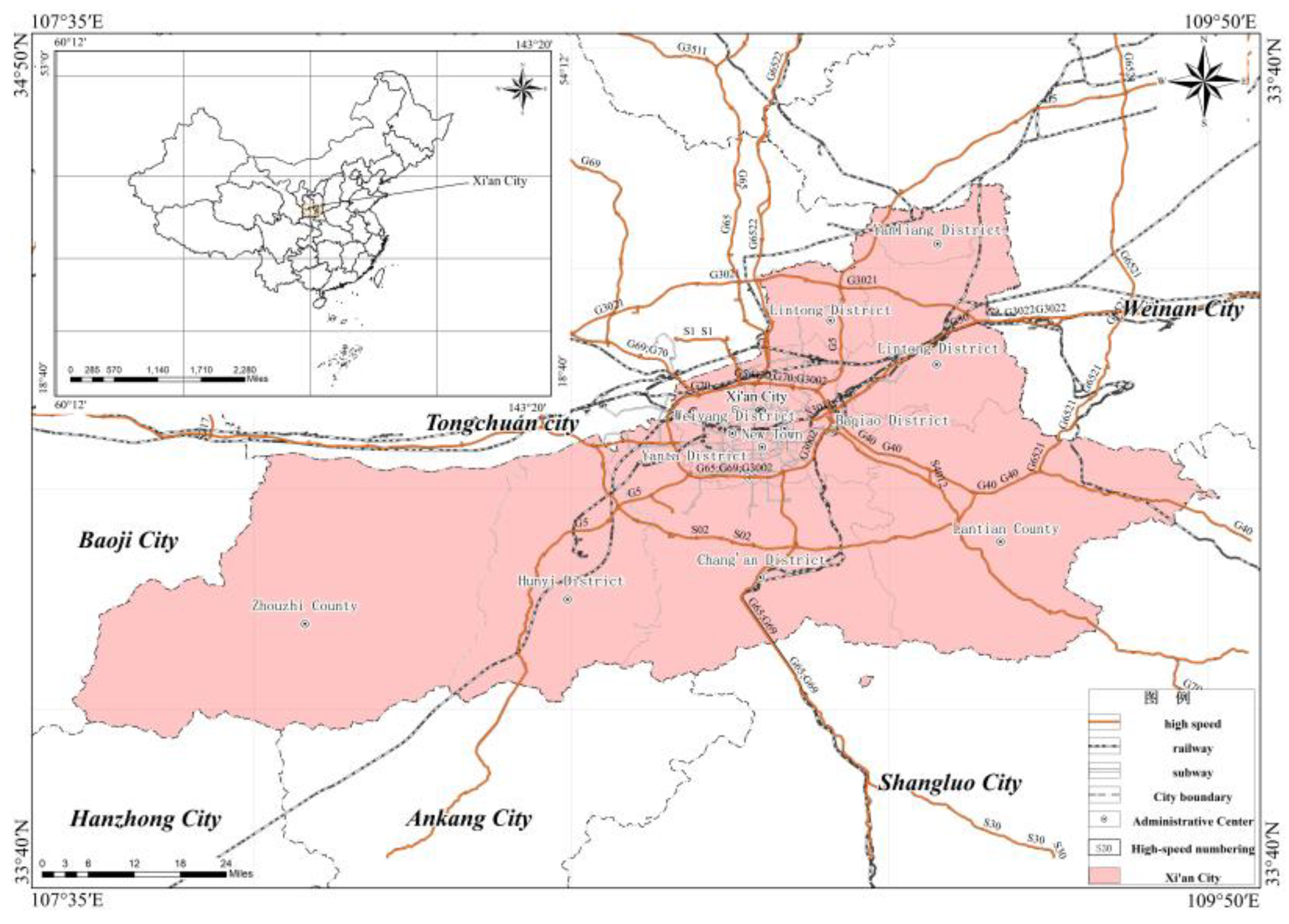
Figure 2.
Distribution Map of Geological Hazard Hidden Danger Points in the Study Area.
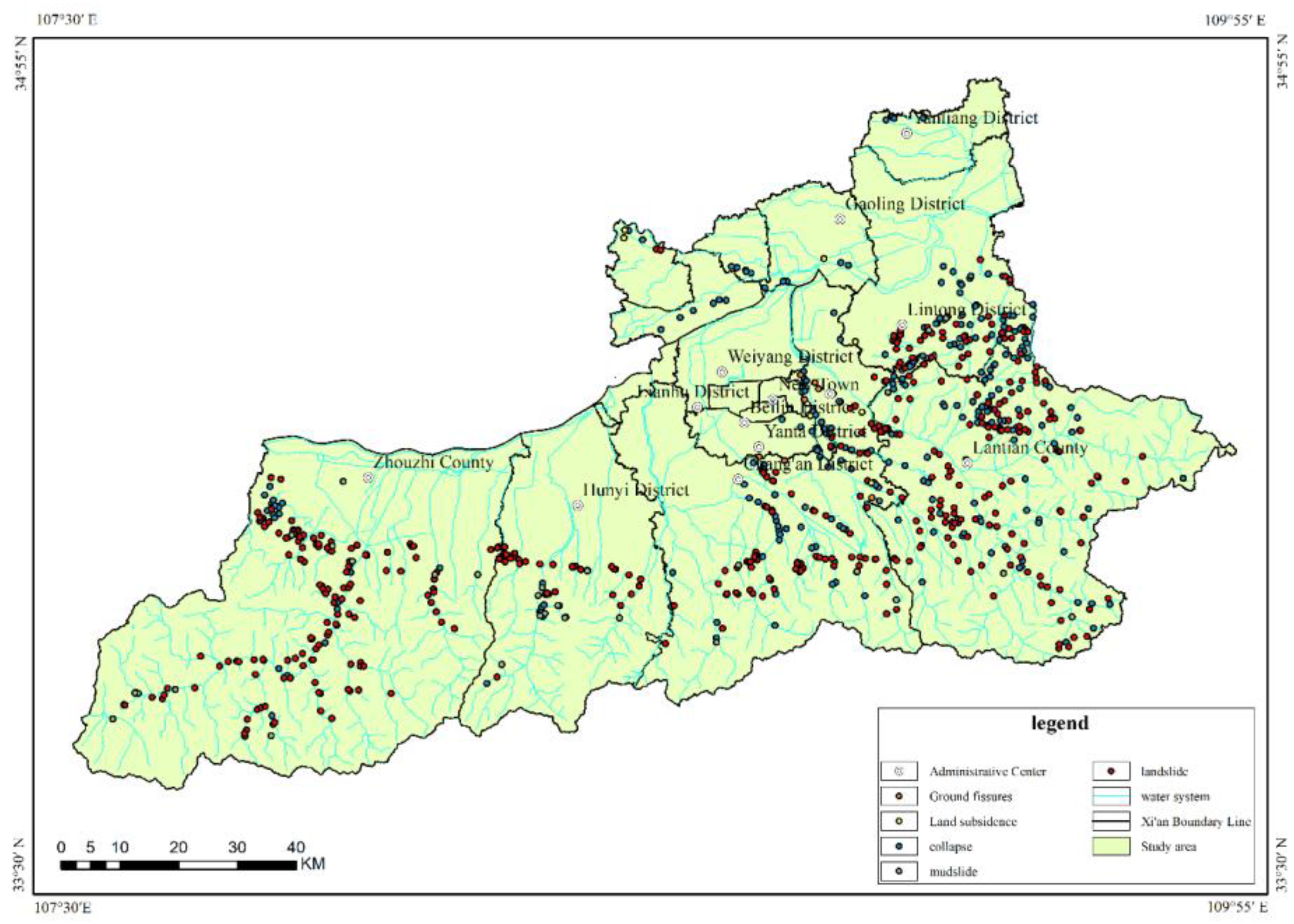
Figure 3.
Ground Subsidence Rate Contour Map of the Study Area.
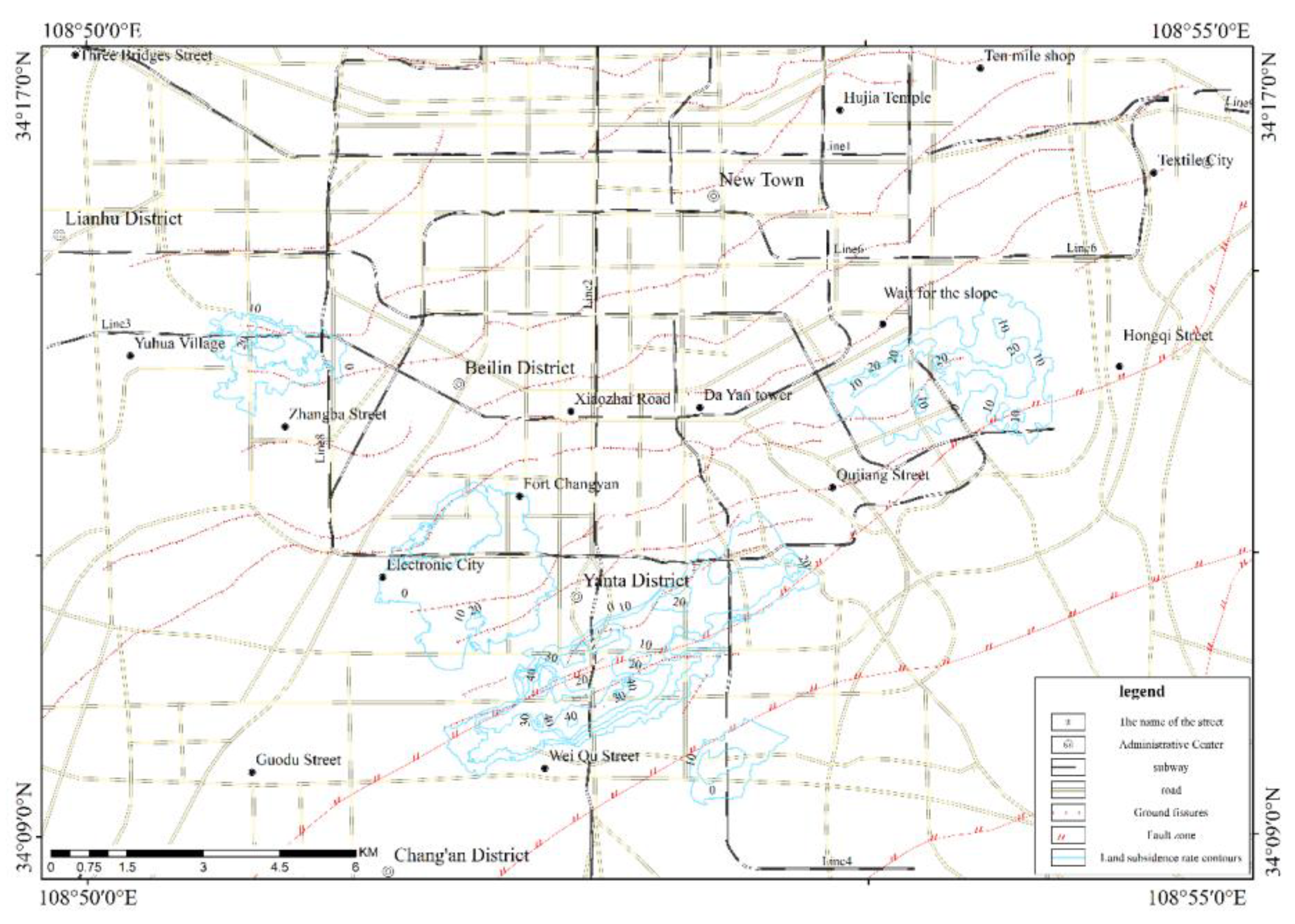
Figure 4.
Cumulative Ground Subsidence Contour Map of the Study Area.
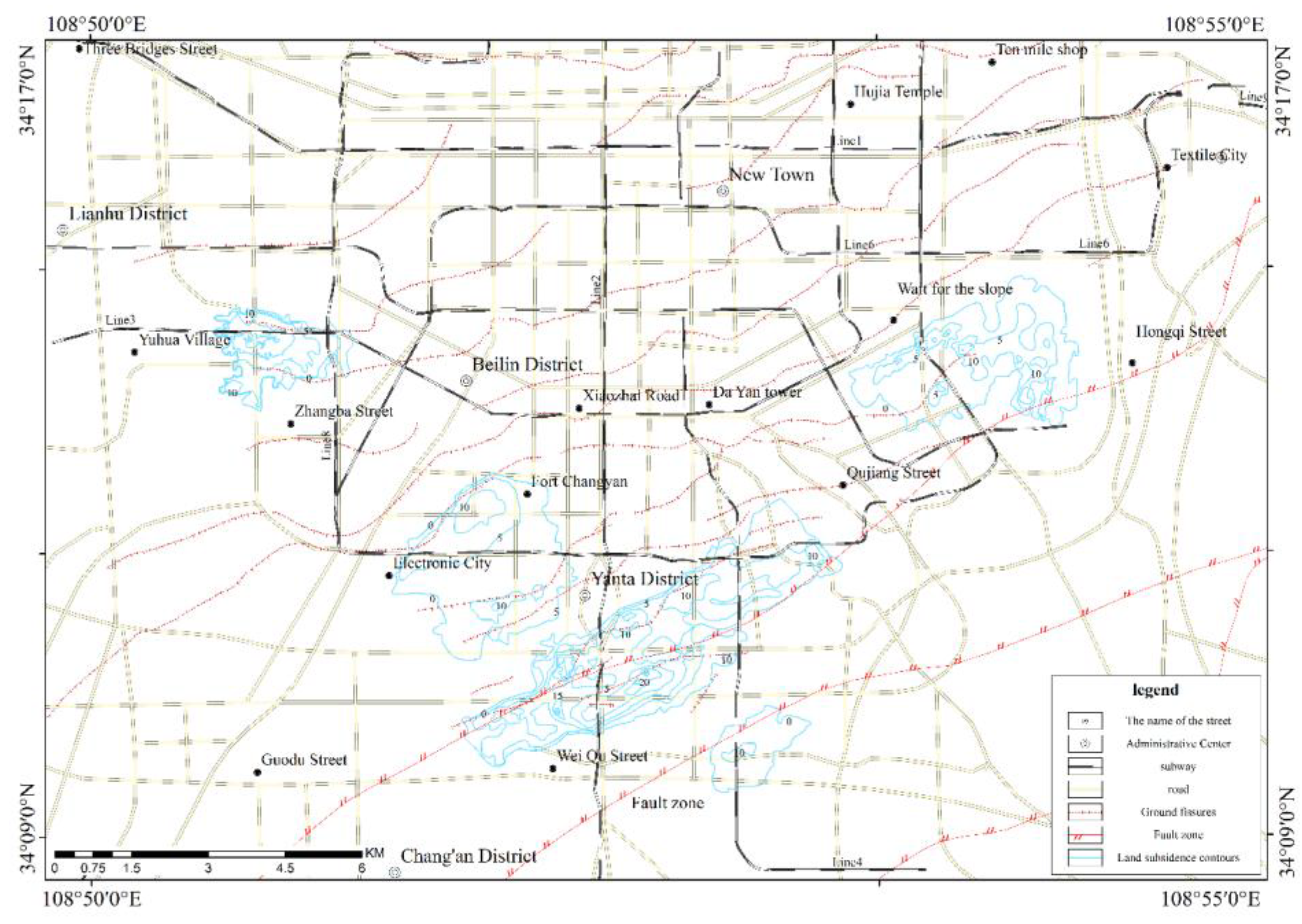
Figure 5.
Relationship Diagram Between the Number of Landslide and Collapse Hazards and Slope Profile Types.
Figure 5.
Relationship Diagram Between the Number of Landslide and Collapse Hazards and Slope Profile Types.
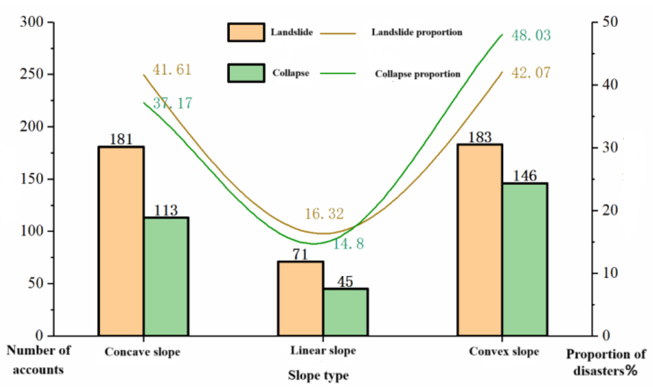
Figure 6.
Relationship Diagram Between the Number of Landslide and Collapse Hazards and Slope Length.
Figure 6.
Relationship Diagram Between the Number of Landslide and Collapse Hazards and Slope Length.
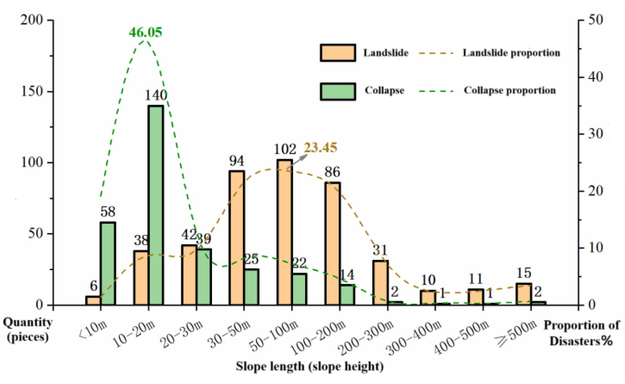
Figure 7.
Relationship Diagram Between the Number of Landslide and Collapse Hazards and Slope Aspect.
Figure 7.
Relationship Diagram Between the Number of Landslide and Collapse Hazards and Slope Aspect.
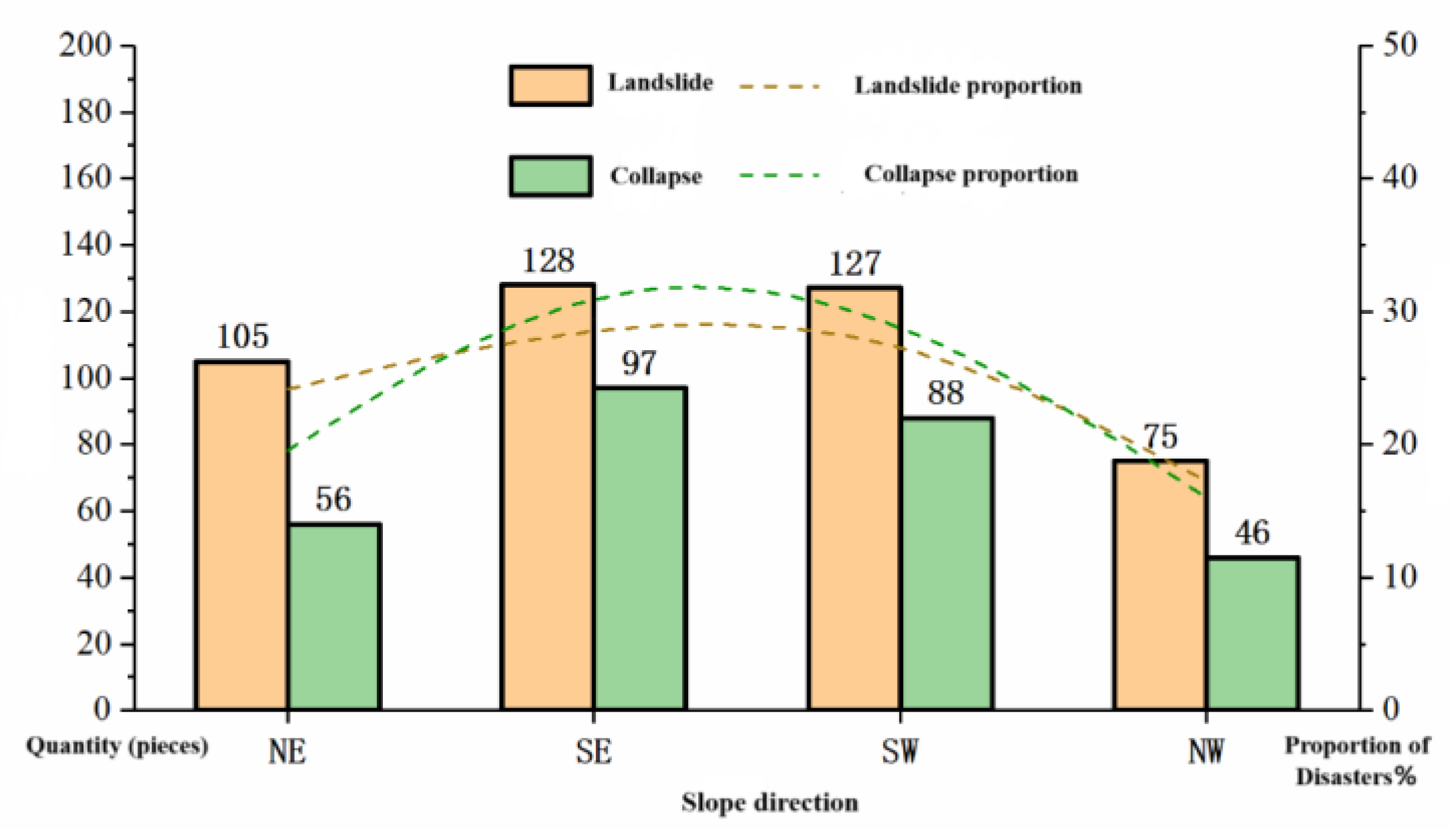
Figure 8.
Relationship Diagram Between the Number of Landslide and Collapse Hazards and Slope Gradient.
Figure 8.
Relationship Diagram Between the Number of Landslide and Collapse Hazards and Slope Gradient.
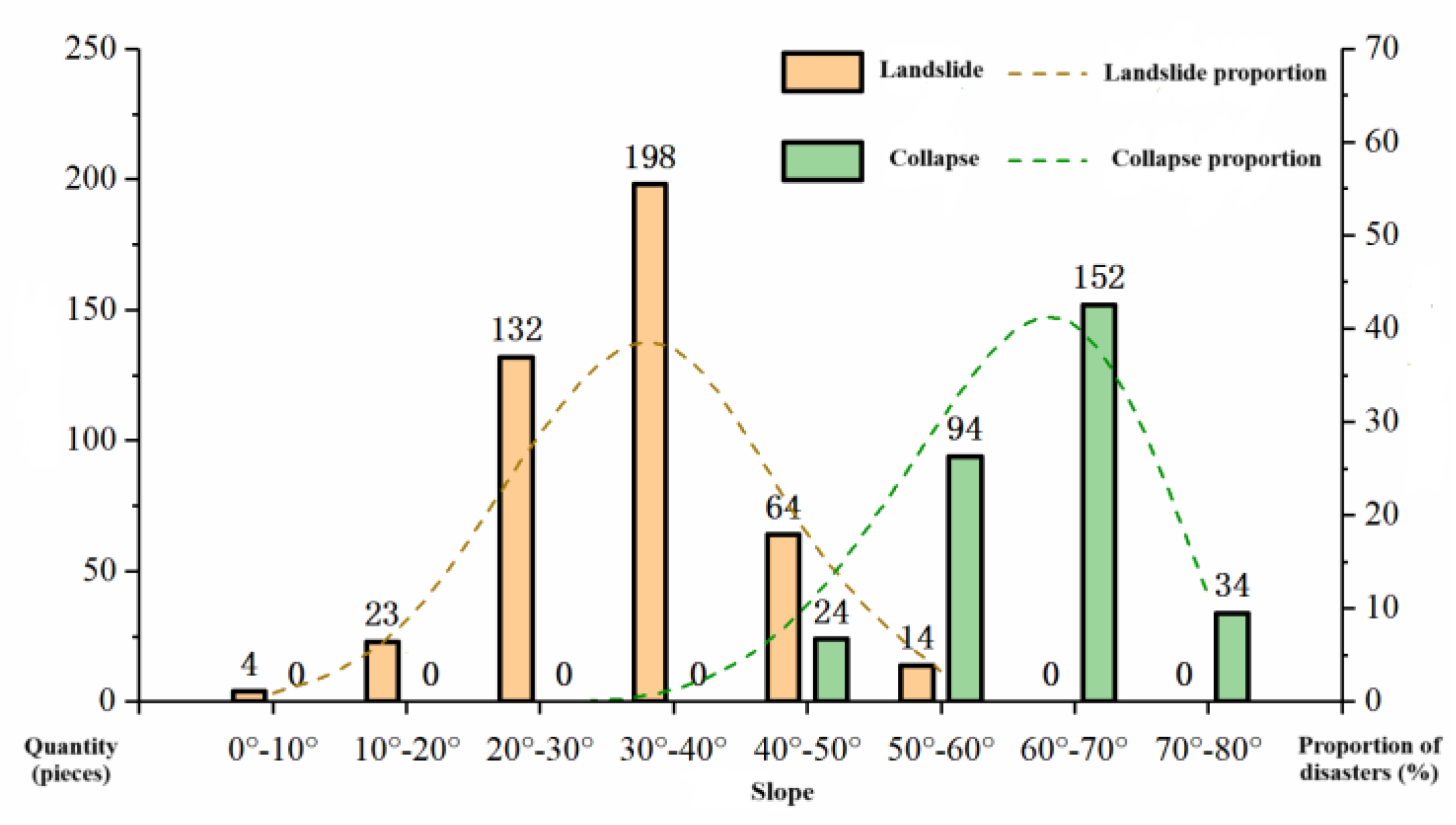
Figure 9.
Schematic Diagram of the Relationship Between Geological Structure and Geological Hazard Distribution.
Figure 9.
Schematic Diagram of the Relationship Between Geological Structure and Geological Hazard Distribution.
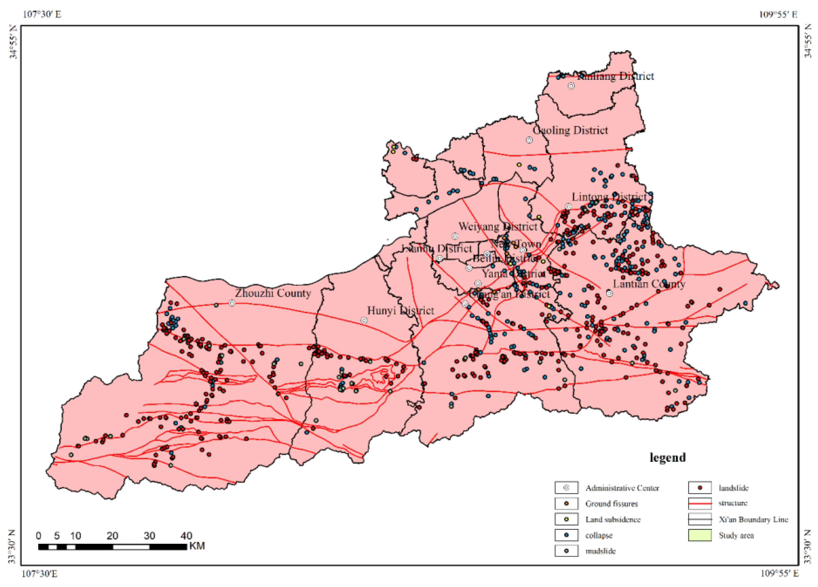
Figure 10.
Geological Hazard Susceptibility Assessment Indicator System.
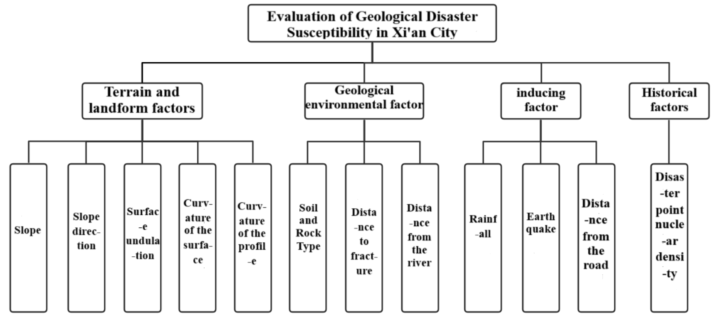
Figure 11.
Slope Gradient Classification Map.
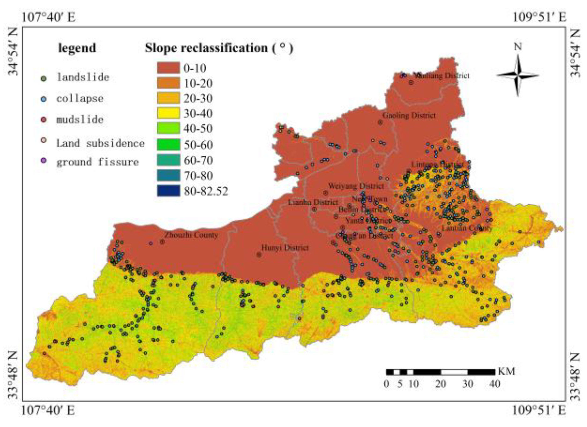
Figure 12.
Slope Aspect Classification Map.
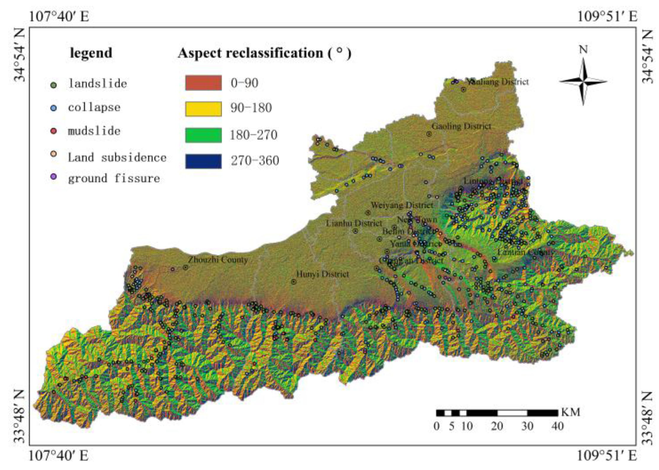
Figure 13.
Surface Relief Classification Map.
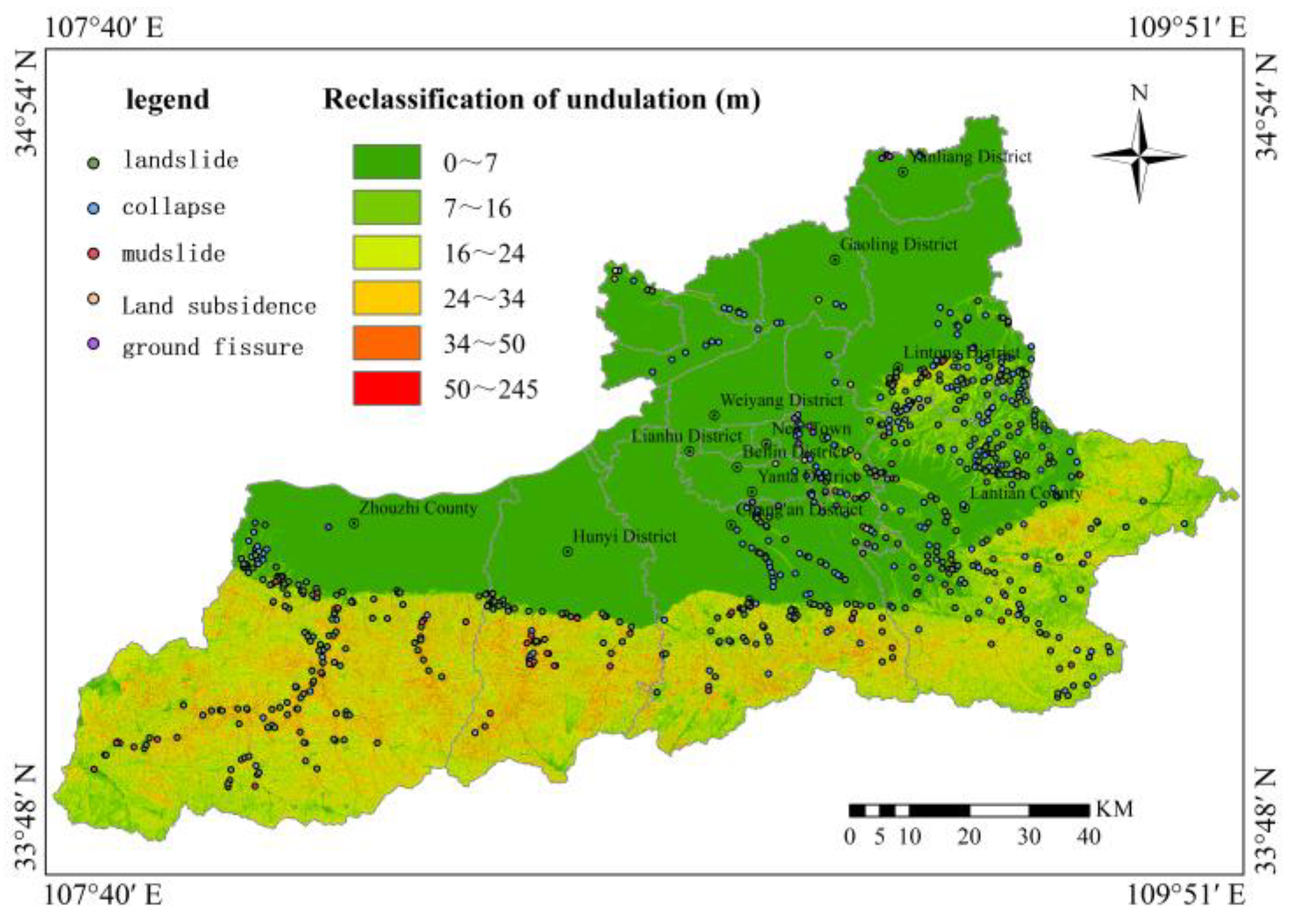
Figure 14.
Plan Curvature Classification Map.
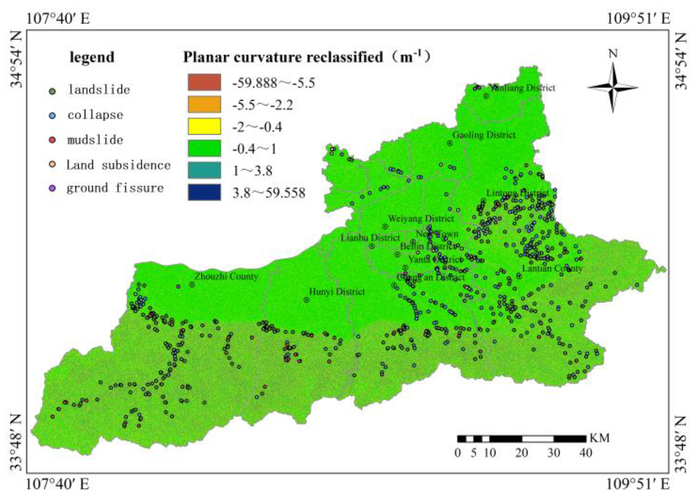
Figure 15.
Profile Curvature Classification Map.
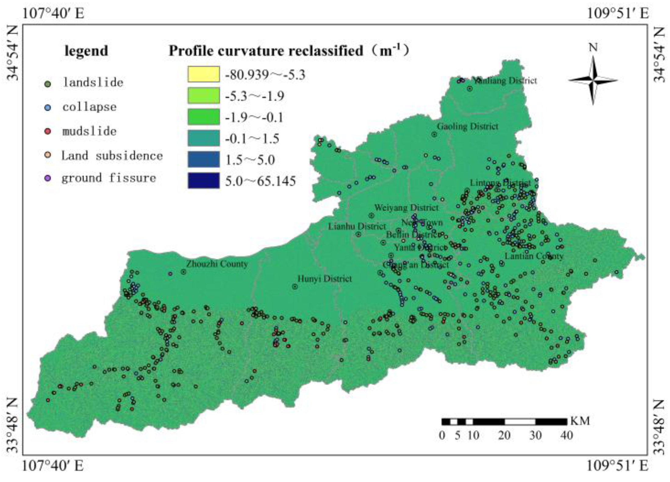
Figure 16.
Rock and Soil Mass Type Classification Map.
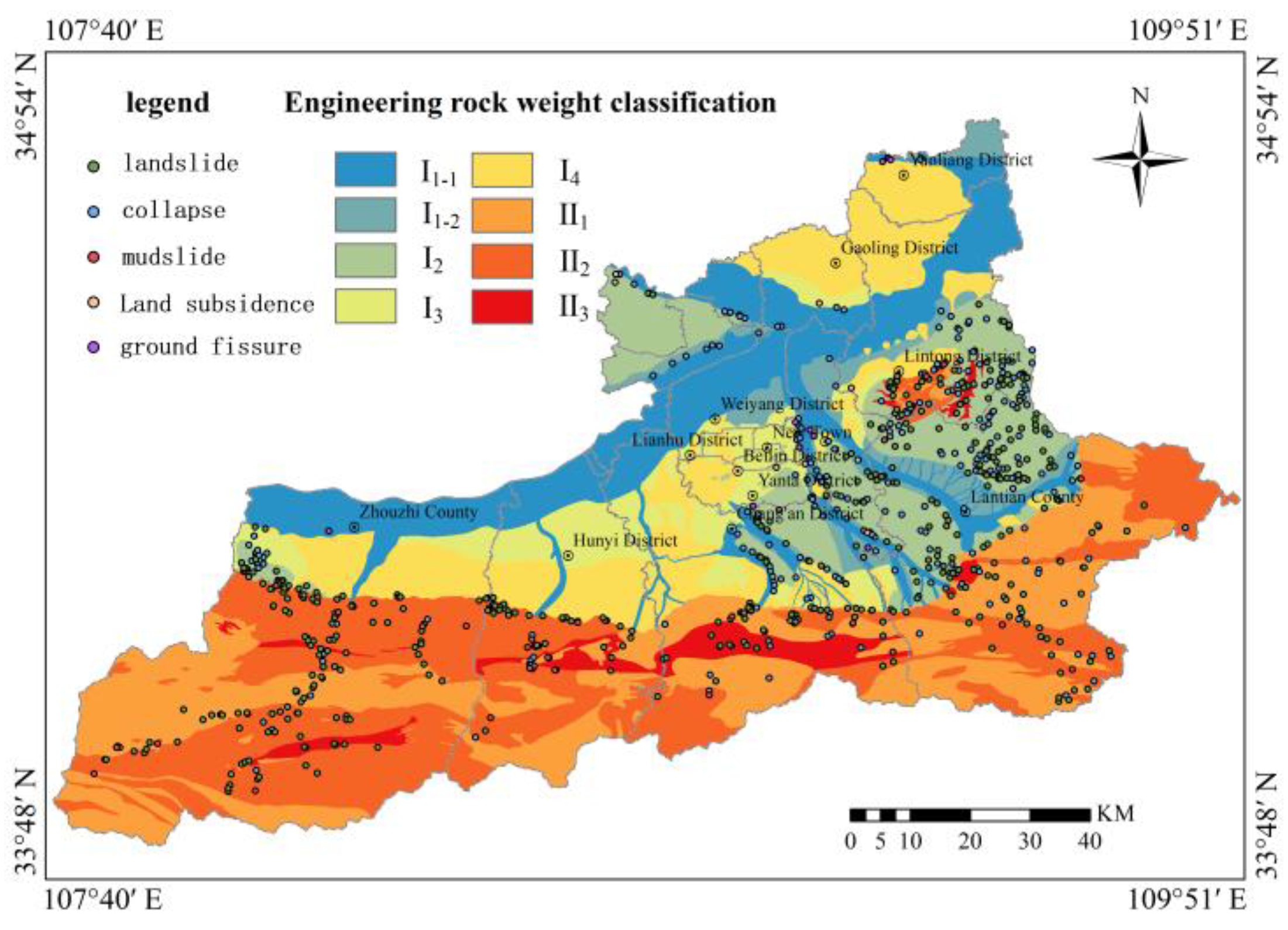
Figure 17.
Distance to Faults Classification Map.
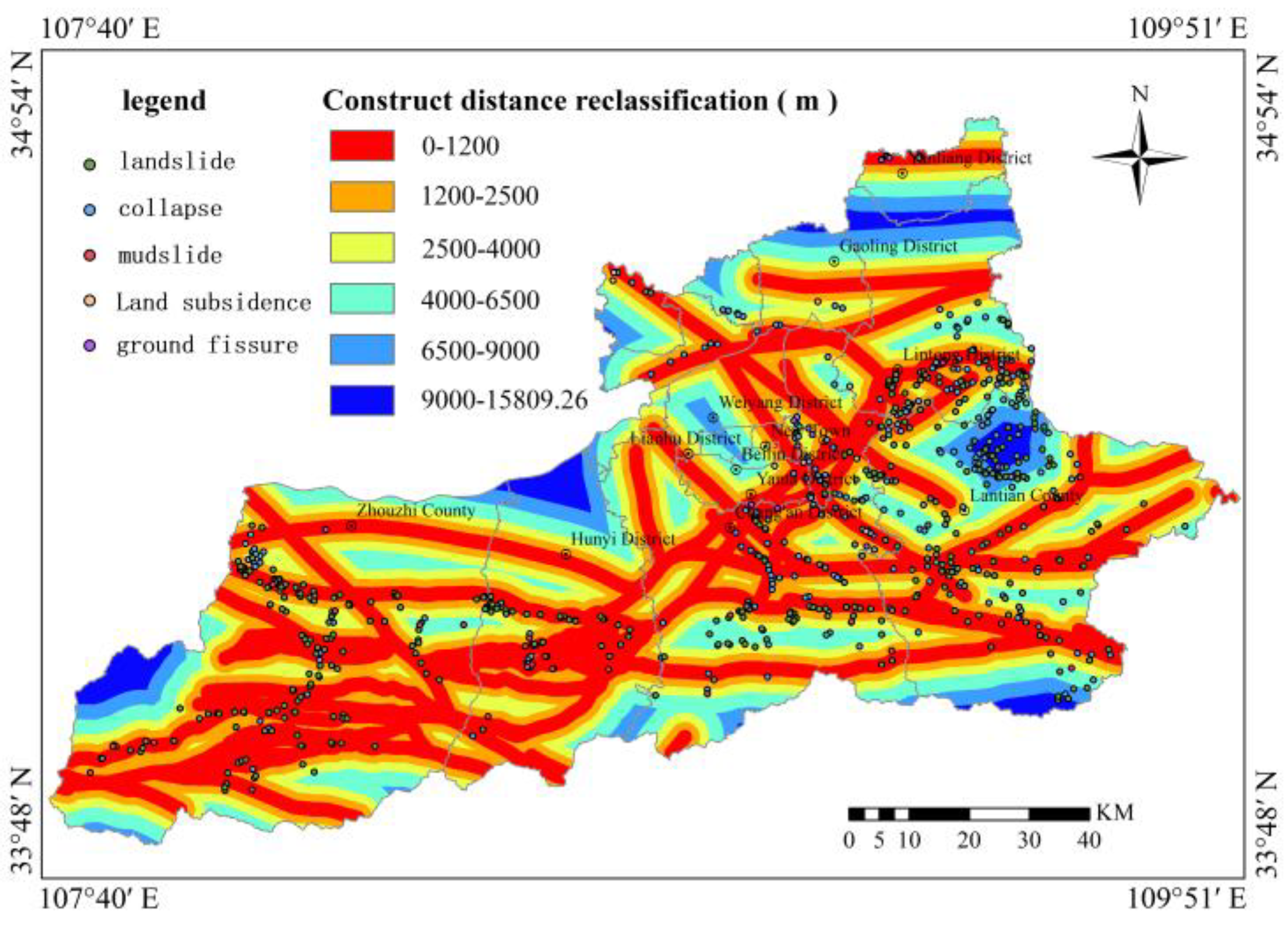
Figure 18.
Distance to Drainage Systems Classification Map.
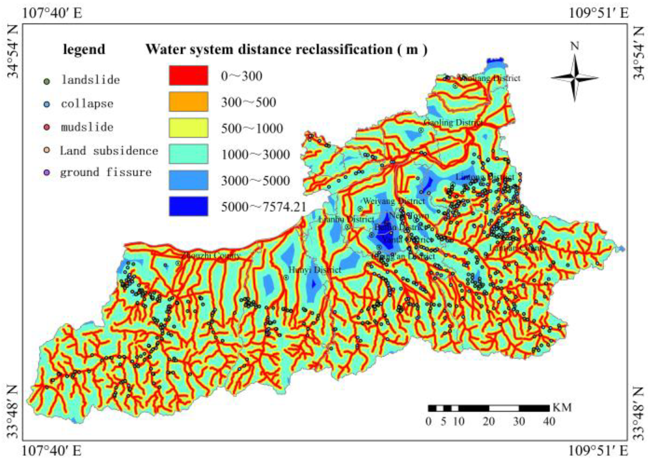
Figure 19.
Rainfall Classification Map.
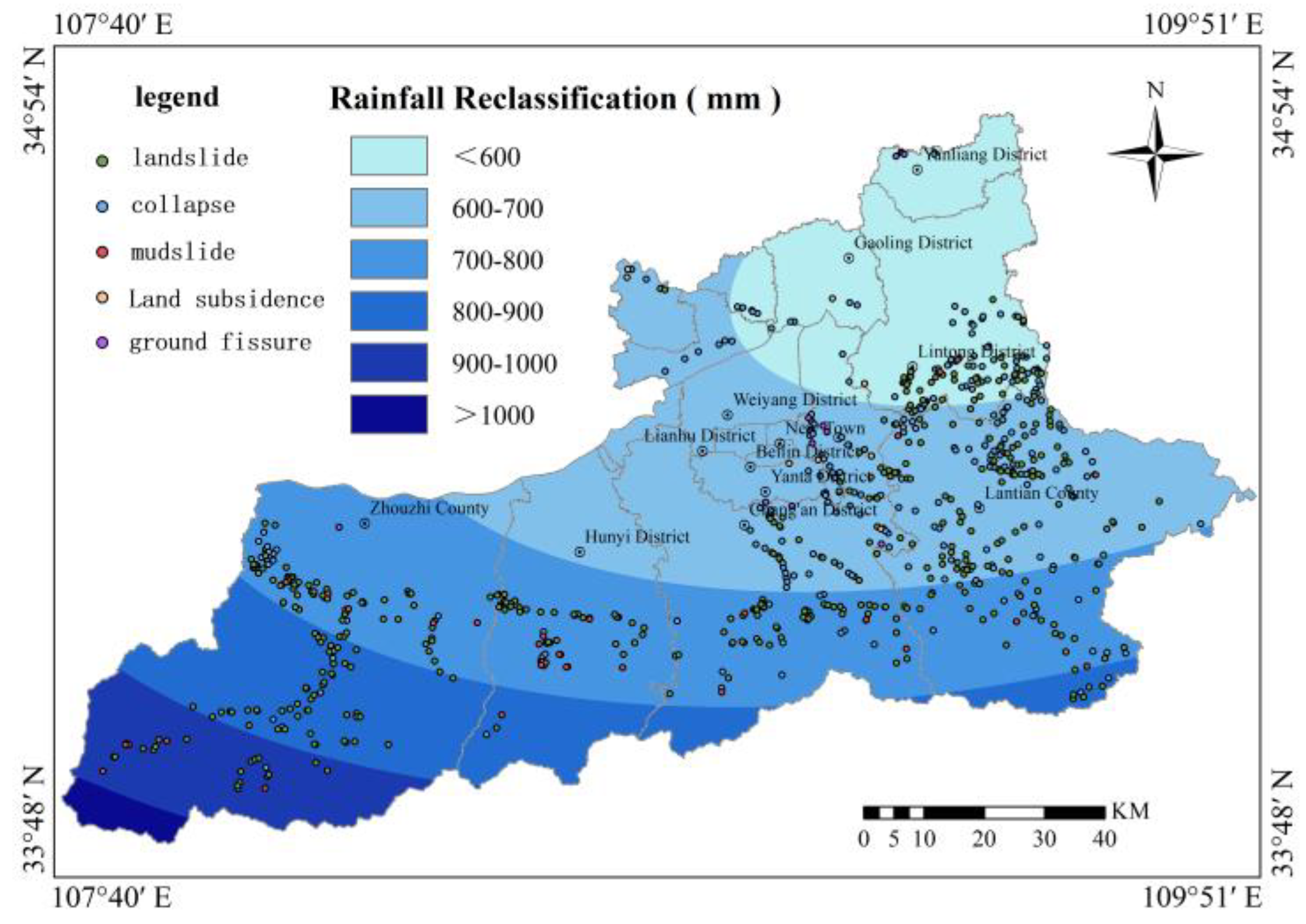
Figure 20.
Seismic Acceleration Classification Map.
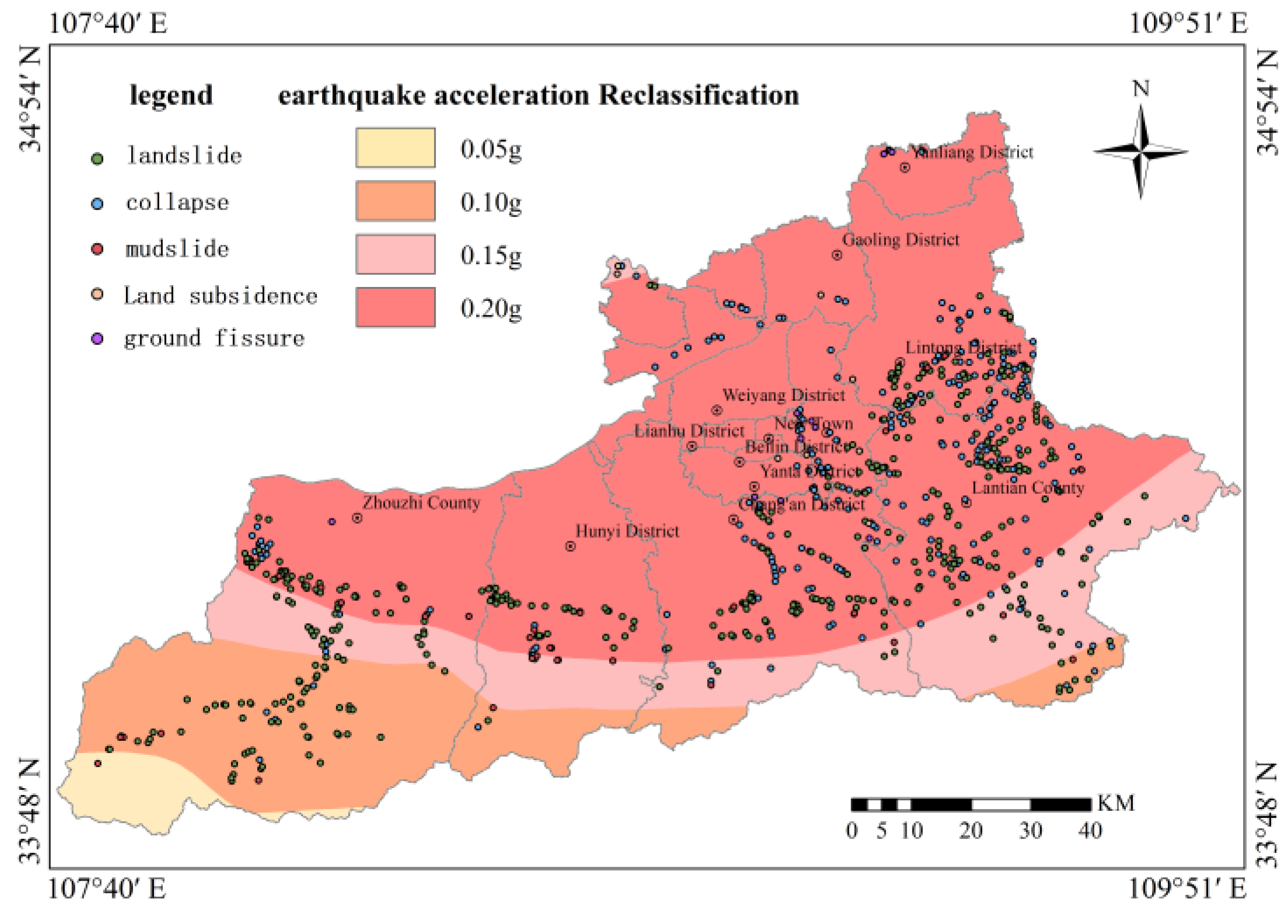
Figure 21.
Distance to Roads Classification Map.
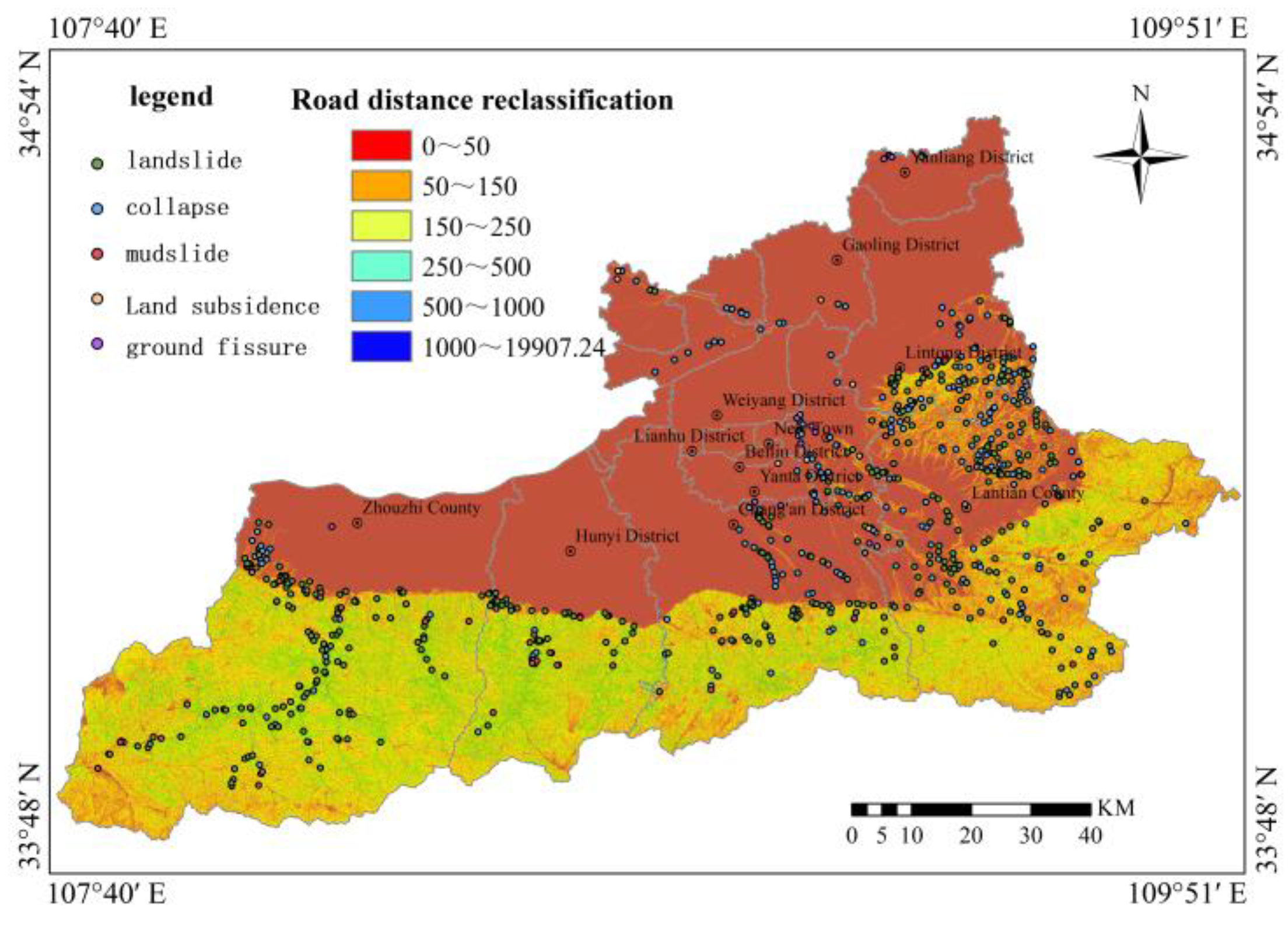
Figure 22.
Hazard Point Kernel Density Classification Map.
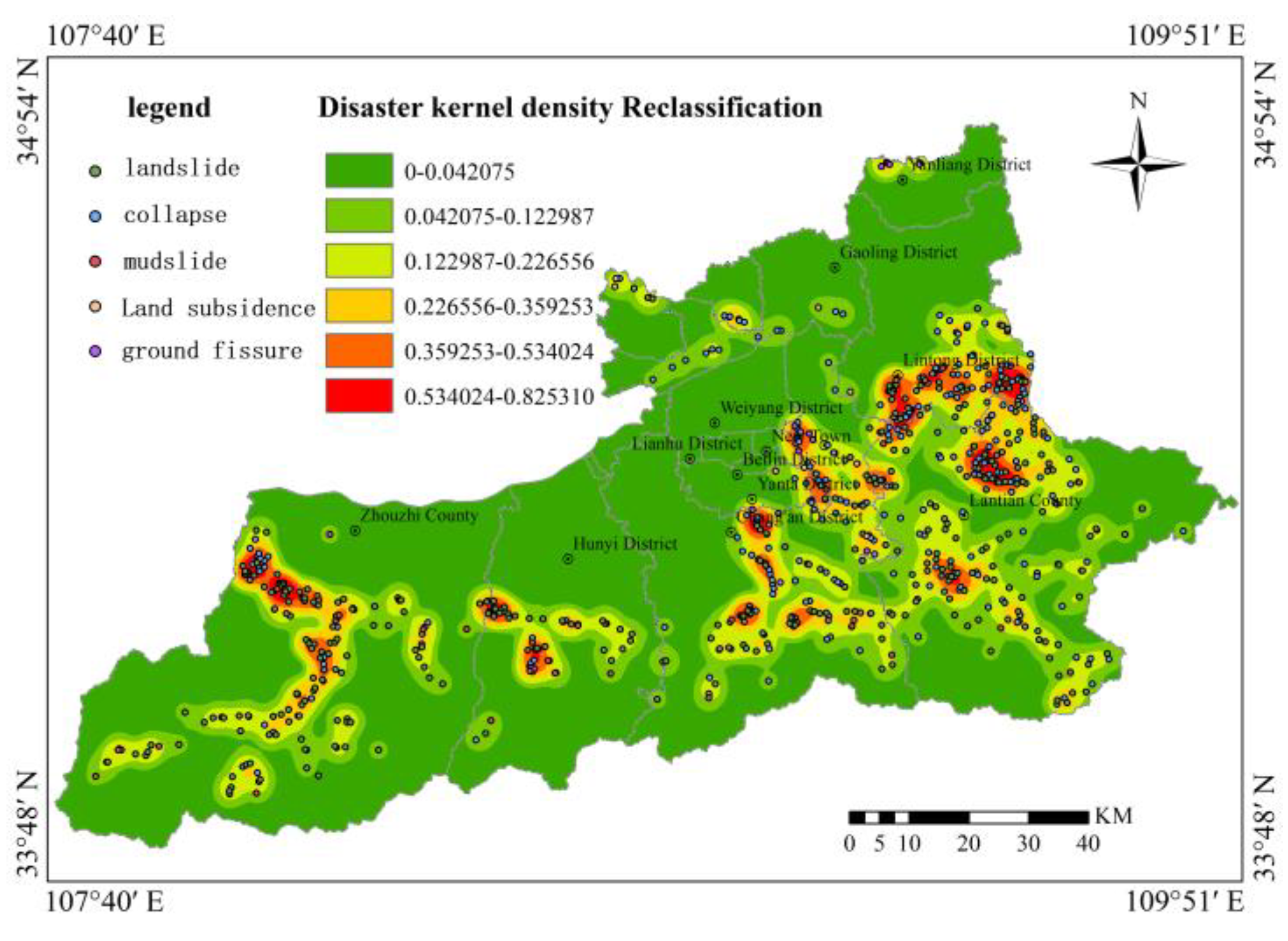
Figure 23.
Schematic Diagram of Analytic Hierarchy Process Hierarchical Model.
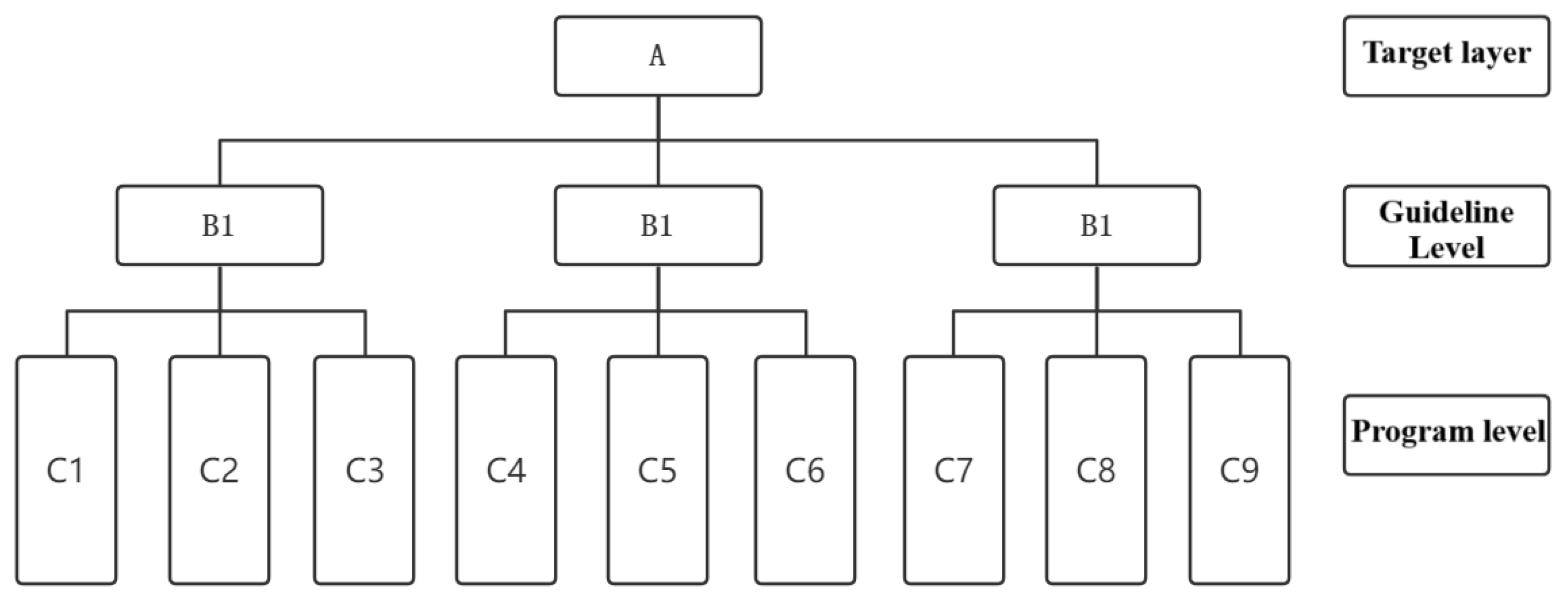
Figure 24.
Analytic Hierarchy Process System Diagram.
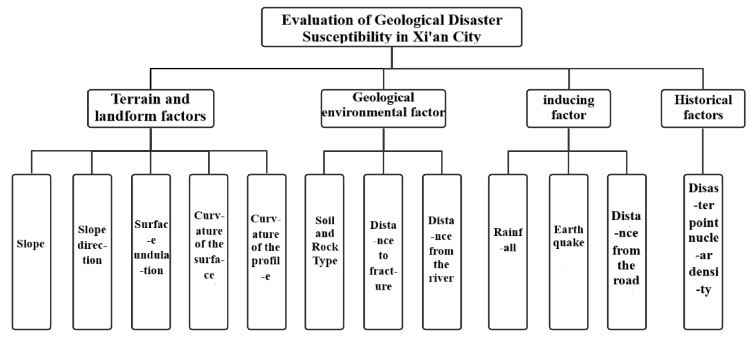
Figure 25.
Evaluation Results Map of Unweighted Information Value Method.

Figure 26.
Evaluation Results Map of Subjective Weighted Information Value Method.
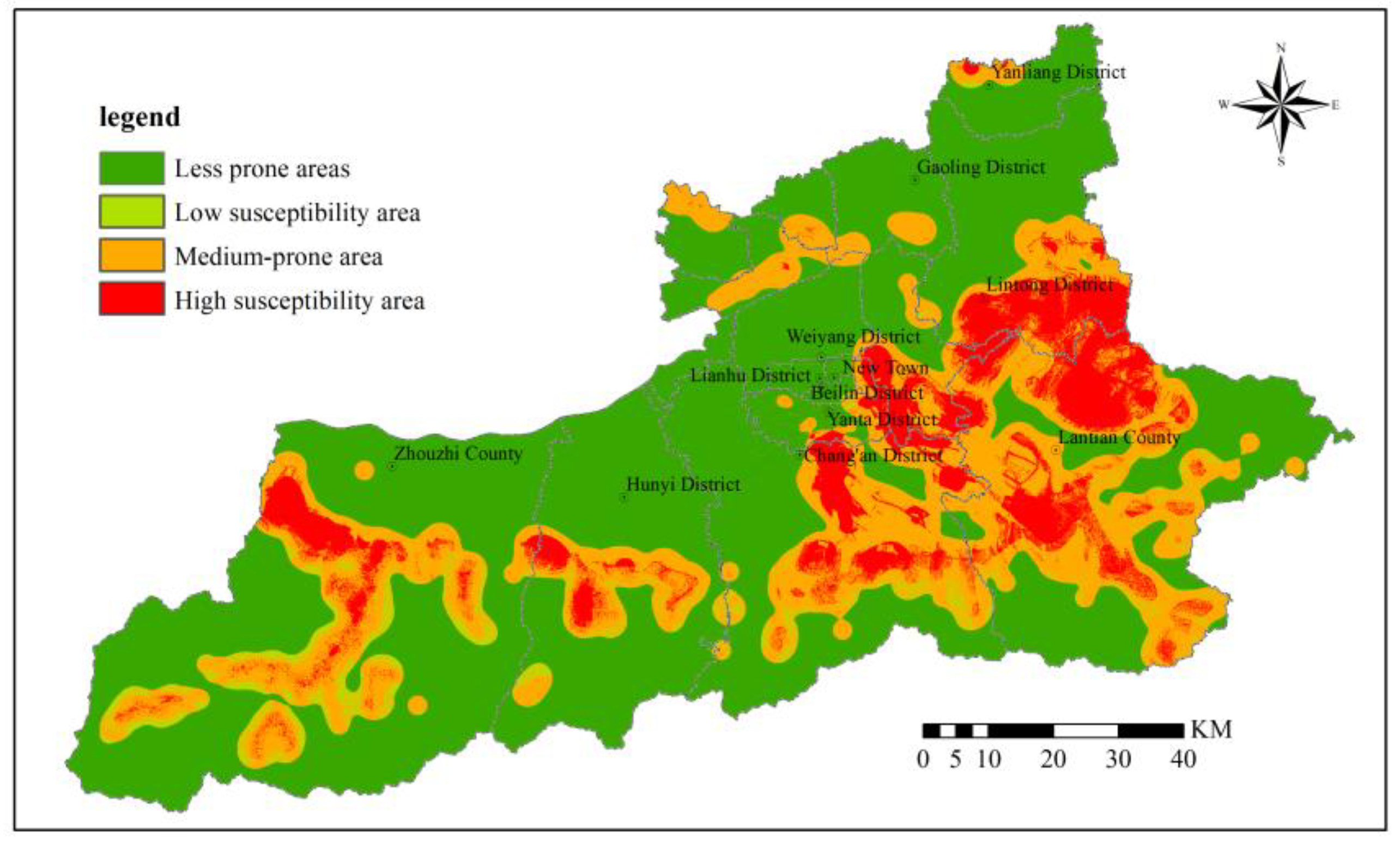
Figure 27.
Evaluation Results Map of Objective Weighted Information Value Method.
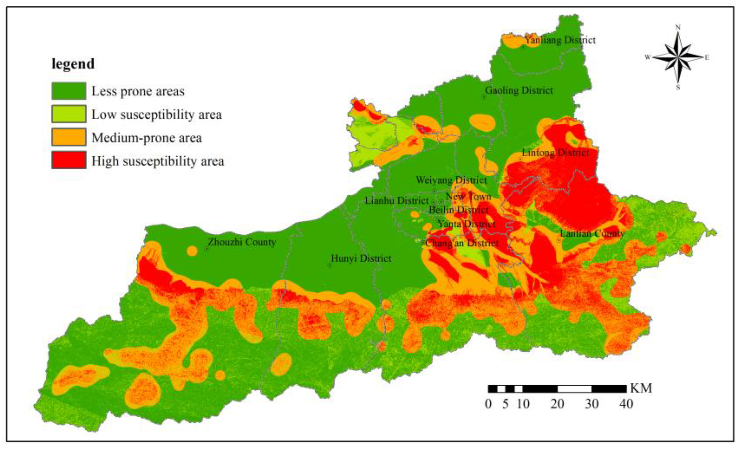
Figure 28.
Evaluation Results Map of Comprehensive Weighted Information Value Method.
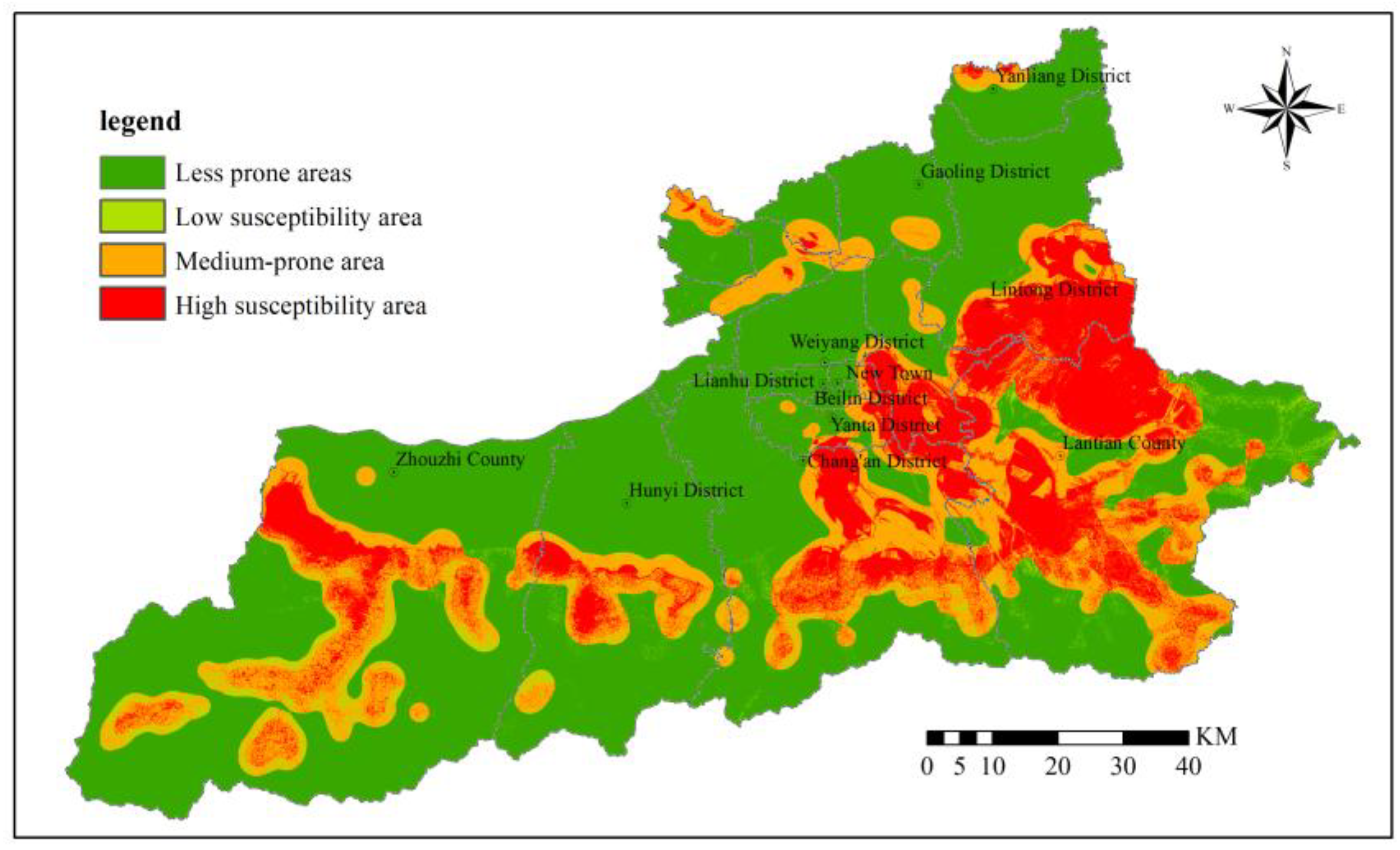
Figure 29.
Comparison of ROC Curves for Different Weighting Models.
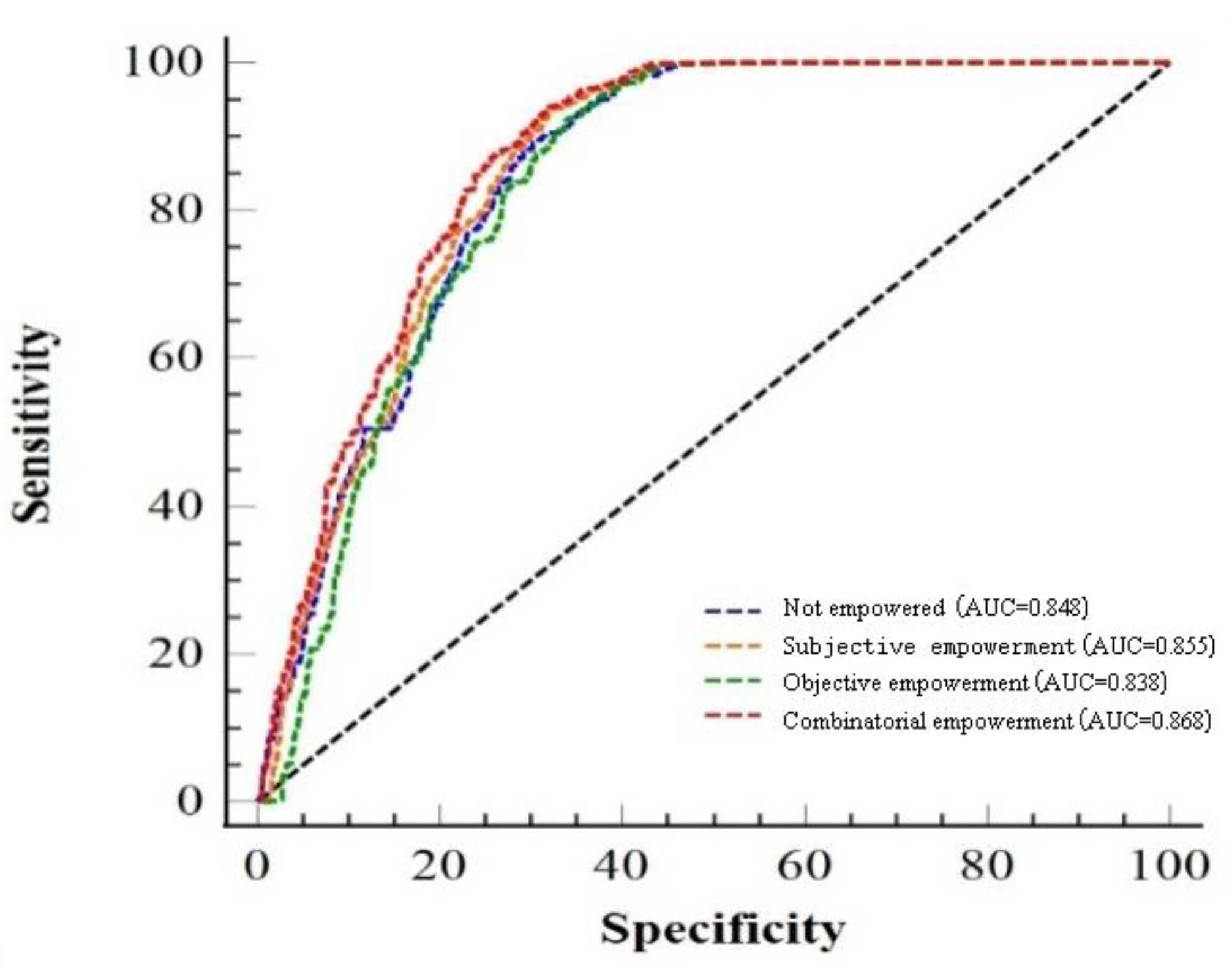

Table 1.
Statistical Table of Sudden-Onset Geological Hazard Types.
| No. | Sudden-Onset Geological Hazards | Classification Criteria | Quantity (Locations) | Percentage | |
| 1 | Landslides | Material Composition | Loess landslides | 206 | 47.36% |
| Accumulation layer landslides | 210 | 48.28% | |||
| Rock landslides | 19 | 4.36% | |||
| Scale | Small | 334 | 76.78% | ||
| Medium | 63 | 14.48% | |||
| Large | 31 | 7.13% | |||
| Extra-large | 6 | 1.38% | |||
| Giant | 1 | 0.23% | |||
| Profile Morphology | Convex | 181 | 41.61% | ||
| Concave | 183 | 42.07% | |||
| Linear | 71 | 16.32% | |||
| 2 | Collapses | Material Composition | Loess collapses | 242 | 79.61% |
| Accumulation layer collapses | 14 | 4.60% | |||
| Rock collapses | 48 | 15.79% | |||
| Scale | Small | 228 | 75.00% | ||
| Medium | 64 | 21.05% | |||
| Large | 10 | 3.29% | |||
| Extra-large | 1 | 0.66% | |||
| 4 | Ground Collapse | Scale Type | Small | 7 | 87.50% |
| Medium | 0 | 0.00% | |||
| Large | 1 | 12.50% | |||
| 3 | Debris Flows | Basin Morphology | Hillslope-type debris flows | 11 | 36.67% |
| Valley-type debris flows | 19 | 63.33% | |||
| Deposit Volume | Small | 21 | 70.00% | ||
| Medium | 8 | 26.67% | |||
| Large | 0 | 0.00% | |||
| Extra-large | 1 | 3.33% | |||
Table 2.
Regional Distribution of Geological Hazard Hidden Danger Points.
| Region | Number of Geological Hazard Hidden Danger Points | Percentage of Total Disaster Points | Disaster Point Quantity Ranking | |||||
| Landslides | Collapses | Debris Flows | Ground Collapse | Ground Fissures | Total | |||
| Lantian County | 122 | 86 | 3 | 0 | 0 | 211 | 26.81% | 1 |
| Zhouzhi County | 144 | 22 | 10 | 0 | 1 | 177 | 22.49% | 2 |
| Chang’an District | 67 | 58 | 6 | 1 | 3 | 135 | 17.15% | 3 |
| Lintong District | 45 | 58 | 2 | 1 | 0 | 106 | 13.47% | 4 |
| Baqiao District | 16 | 40 | 0 | 1 | 4 | 61 | 7.75% | 5 |
| Huyi County | 37 | 8 | 9 | 0 | 0 | 54 | 6.86% | 6 |
| Xixian New Area | 4 | 13 | 0 | 2 | 0 | 19 | 2.41% | 7 |
| Yanliang District | 0 | 6 | 0 | 0 | 2 | 8 | 1.02% | 8 |
| Gaoling District | 0 | 5 | 0 | 1 | 0 | 6 | 0.76% | 9 |
| Chanba Ecological District | 0 | 4 | 0 | 1 | 0 | 5 | 0.64% | 10 |
| Yanta District | 0 | 3 | 0 | 1 | 0 | 4 | 0.51% | 11 |
| International Port District | 0 | 1 | 0 | 0 | 0 | 1 | 0.13% | 12 |
| Total | 435 | 304 | 30 | 8 | 10 | 787 | — | — |
Table 3.
Relationship Table Between Geological Hazard Quantities and Geomorphological Types.
| Hazard Type | Number of Hazard Points | Total | |||
| Alluvial, Alluvial-Pluvial Plains | Piedmont Pluvial Plain Areas | Loess Landform Areas | Mountainous Regions | ||
| Landslides | 31 | 5 | 136 | 263 | 435 |
| Collapses | 61 | 17 | 150 | 76 | 304 |
| Debris Flows | - | 1 | 2 | 27 | 30 |
| Ground Collapse | 6 | - | 2 | - | 8 |
| Ground Fissures | 8 | - | 2 | - | 10 |
| Total | 106 | 23 | 292 | 366 | 787 |
Table 4.
Statistical Table of Relationships Between Geomorphological Types and Geological Hazards.
| Geomorphological Type | Area(km2) | Geological Hazard Points | |
| Number | Percentage | ||
| Alluvial, Alluvial-Pluvial Plain Areas | 3188.08 | 106 | 13.47% |
| Piedmont Pluvial Plain Areas | 873.96 | 23 | 2.92% |
| Loess Landform Areas | 1279.10 | 292 | 37.10% |
| Mountainous Regions | 5248.20 | 366 | 46.51% |
Table 5.
Statistical Table of Distribution Quantities of Geological Hazard Hidden Danger Points in Different Stratigraphic Ages.
Table 5.
Statistical Table of Distribution Quantities of Geological Hazard Hidden Danger Points in Different Stratigraphic Ages.
| Stratigraphic Age | Landslides | Collapses | Debris Flows | Ground Collapse | Ground Fissures | Total | Percentage |
| Quaternary | 156 | 173 | 5 | 8 | 10 | 352 | 44.73% |
| Neogene | 32 | 23 | 0 | 0 | 0 | 55 | 6.99% |
| Paleogene | 32 | 46 | 1 | 0 | 0 | 79 | 10.04% |
| Upper Paleozoic | 41 | 14 | 4 | 0 | 0 | 59 | 7.50% |
| Middle Paleozoic | 18 | 1 | 1 | 0 | 0 | 20 | 2.54% |
| Lower Paleozoic | 68 | 19 | 9 | 0 | 0 | 96 | 12.19% |
| Proterozoic | 73 | 14 | 10 | 0 | 0 | 97 | 12.33% |
| Neoarchean | 15 | 14 | 0 | 0 | 0 | 29 | 3.68% |
| Total | 435 | 304 | 30 | 8 | 10 | 787 | — |
Table 6.
Statistical Table of Geological Hazard Quantities in Different Rock and Soil Mass Zones.
| Rock and Soil Mass Zone Code | Area(km2) | Geological Hazard Types | ||||
| Collapses | Landslides | Debris Flows | Ground Collapse | Ground Fissures | ||
| Silty clay + sandy gravel dual-layer structure zone (I1-1) | 1721.61 | 40 | 12 | - | 1 | 2 |
| Loess (interbedded with paleosol) + sand, sandy gravel dual-layer structure zone (I1-2) | 410.78 | 25 | 19 | - | 1 | 2 |
| Loess (interbedded with paleosol) single-layer structure zone (I2) | 1291.64 | 148 | 139 | 3 | 3 | 2 |
| Loess, loess-like soil and sandy gravel multi-layer structure zone (I3) | 717.93 | 11 | 5 | - | 3 | 2 |
| Sandy gravel, sandy clay multi-layer structure zone (I4) | 1416.82 | 7 | 9 | 2 | - | 2 |
| Massive hard intrusive rock engineering geological zone (II1) | 2236.67 | 30 | 80 | 8 | - | - |
| Massive hard to moderately hard intermediate to high-grade metamorphic rock engineering geological zone (II2) | 2451.27 | 35 | 143 | 16 | - | - |
| Layered moderately hard to weak sedimentary rock engineering geological zone (II3) | 342.17 | 8 | 28 | 1 | - | - |
| Total | 10588.9 | 304 | 435 | 30 | 10 | 8 |
Table 7.
Correlation Analysis Results of Assessment Factors.
| A | B | C | D | E | F | G | H | I | J | K | L | M | |
| A | 1.000 | 0.421 | 0.003 | 0.434 | -0.015 | 0.028 | 0.613 | 0.095 | -0.15 | 0.479 | -0.557 | 0.115 | -0.012 |
| B | 1.000 | -0.041 | 0.481 | 0.05 | 0.035 | 0.482 | -0.096 | -0.23 | 0.359 | -0.31 | -0.016 | -0.037 | |
| C | 1.000 | -0.043 | 0.017 | 0.007 | 0.007 | -0.025 | 0.049 | -0.075 | 0.048 | -0.019 | 0.075 | ||
| D | 1.000 | 0.043 | 0.041 | 0.492 | -0.099 | -0.225 | 0.373 | -0.332 | -0.015 | -0.047 | |||
| E | 1.000 | -0.44 | 0.002 | -0.06 | -0.037 | -0.05 | 0.018 | -0.011 | -0.016 | ||||
| F | 1.000 | 0.054 | 0.06 | -0.063 | 0.046 | -0.093 | -0.067 | 0.041 | |||||
| G | 1.000 | -0.135 | -0.263 | 0.48 | -0.483 | 0.027 | -0.123 | ||||||
| H | 1.000 | -0.076 | -0.128 | 0.143 | 0.047 | -0.001 | |||||||
| I | 1.000 | -0.31 | 0.312 | 0.148 | 0.218 | ||||||||
| J | 1.000 | -0.423 | 0.073 | -0.208 | |||||||||
| K | 1.000 | 0.06 | 0.357 | ||||||||||
| L | 1.000 | -0.003 | |||||||||||
| M | 1.000 |
Note: A represents elevation, B represents slope gradient, C represents slope aspect, D represents surface relief, E represents plan curvature, F represents profile curvature, G represents rock and soil mass types, H represents distance to faults, I represents distance to drainage systems, J represents rainfall, K represents earthquake intensity, L represents distance to roads, M represents kernel density.
Table 8.
Classification and Statistical Table of Geological Hazard Influencing Factors.
| Influencing Factor | Classification | Area (km2) | Hazard Points | Influencing Factor | Classification | Area (km2) | Hazard Points |
| Slope Gradient (°) | 0~10 | 5231.6 | 4 | Rock and Soil Mass Types | I1-1 | 1721.59 | 55 |
| 10~20 | 1157.62 | 23 | I1-2 | 410.78 | 47 | ||
| 20~30 | 1610.37 | 132 | I2 | 1291.66 | 295 | ||
| 30~40 | 1616.81 | 198 | I3 | 717.94 | 21 | ||
| 40~50 | 794.215 | 88 | I4 | 1416.83 | 20 | ||
| 50~60 | 171.923 | 108 | II1 | 2236.68 | 118 | ||
| 60~70 | 23.43 | 152 | II2 | 2469.88 | 194 | ||
| 70~80 | 1.558 | 34 | II3 | 342.17 | 37 | ||
| 80~90 | 0.006 | 0 | Distance to Faults (m) | 0~1200 | 3638.99 | 388 | |
| Slope Aspect (°) | 0~90 | 3390.9 | 177 | 1200~2500 | 2533.83 | 170 | |
| 90~180 | 2322.28 | 238 | 2500~4000 | 1913.14 | 87 | ||
| 180~270 | 2399.08 | 237 | 4000~6500 | 1586.72 | 77 | ||
| 270~360 | 2495.27 | 135 | 6500~9000 | 616.76 | 41 | ||
| Surface Relief | 0~7 | 5484.441 | 332 | 9000~15809.26 | 318.08 | 24 | |
| 7~16 | 1916.21 | 324 | Hazard Point Kernel Density (points/km2) | 0~0.042 | 6501.6 | 1 | |
| 16~24 | 1744.91 | 92 | 0.042~0.123 | 1823.72 | 90 | ||
| 24~34 | 1079.1 | 27 | 0.123~0.227 | 1237.4 | 196 | ||
| 34~50 | 335.071 | 10 | 0.227~0.359 | 602.78 | 189 | ||
| 50~245 | 47.798 | 2 | 0.359~0.534 | 312.78 | 179 | ||
| Rainfall (mm) | <600 | 3638.99 | 130 | 0.534~0.825 | 129.25 | 132 | |
| 600~700 | 2533.83 | 302 | Plan Curvature | -59.888~-5.5 | 71.3602 | 2 | |
| 700~800 | 1913.14 | 260 | -5.5~-2.2 | 430.265 | 31 | ||
| 800~900 | 1586.72 | 70 | -2.2~-0.4 | 2513.08 | 221 | ||
| 900~1000 | 616.76 | 25 | -0.4~1 | 6170.73 | 426 | ||
| >1000 | 318.08 | 0 | 1~3.8 | 1232.8 | 95 | ||
| 3.5~59.558 | 189.296 | 12 | |||||
| Distance to Drainage Systems | 0~300 | 2261.27 | 240 | Profile Curvature | -80.939~-5.3 | 145.699 | 6 |
| 300~500 | 1355.63 | 110 | -5.3~-1.9 | 576.348 | 49 | ||
| 500~1000 | 2853.92 | 201 | -1.9~-0.1 | 3547.06 | 235 | ||
| 1000~3000 | 3662.43 | 220 | -0.1~1.5 | 5379.03 | 398 | ||
| 3000~5000 | 416.032 | 15 | 1.5~5.0 | 791.59 | 91 | ||
| 5000~7574.21 | 58.2366 | 1 | 5.0~65.145 | 167.804 | 8 | ||
| Earthquake | <0.05 | 264.796 | 1 | Distance to Roads | 0~50 | 304.462 | 56 |
| 0.05~0.10 | 1826.71 | 87 | 50~150 | 581.768 | 104 | ||
| 0.10~0.20 | 1637.64 | 80 | 150~250 | 511.704 | 83 | ||
| >0.20 | 6878.37 | 619 | 250~500 | 1101 | 156 | ||
| 500~1000 | 1641.95 | 169 | |||||
| >1000 | 6466.64 | 219 |
Table 9.
Scale Values and Their Meanings.
| Scale(Cij) | Meaning |
| 1 | Factors i and j are equally important |
| 3 | Factor i is slightly more important than factor j |
| 5 | Factor i is obviously more important than factor j |
| 7 | Factor i is strongly more important than factor j |
| 9 | Factor i is extremely more important than factor j |
| 2、4、6、8 | Importance levels are in intermediate states |
| Reciprocals of the above scale values | Represent the degree of importance of factor j compared to factor i |
Table 10.
Judgment Matrix C.
| C | C1 | C2 | C3 | …… | Cn |
| C1 | c11 | c12 | c13 | …… | c1n |
| C2 | c21 | c22 | c23 | …… | c2n |
| C3 | c31 | c32 | c33 | …… | c3n |
| …… | …… | …… | …… | …… | …… |
| Cn | cn1 | cn2 | cn3 | …… | cnn |
Table 11.
Weight Coefficient Values via Analytic Hierarchy Process.
| Indicator | A | B | C | D | E | F | G | H | I | J | K | L |
| Weight | 0.102 | 0.018 | 0.102 | 0.018 | 0.018 | 0.040 | 0.070 | 0.029 | 0.131 | 0.055 | 0.170 | 0.247 |
Note: A represents slope gradient, B represents slope aspect, C represents surface relief, D represents plan curvature, E represents profile curvature, F represents rock and soil mass types, G represents distance to faults, H represents distance to drainage systems, I represents rainfall, J represents earthquake intensity, K represents distance to roads, L represents hazard point kernel density.
Table 12.
Weight Coefficient Values via Entropy Weight Method.
| Indicator | A | B | C | D | E | F | G | H | I | J | K | L |
| Weight | 0.137 | 0.124 | 0.163 | 0.017 | 0.018 | 0.145 | 0.026 | 0.009 | 0.193 | 0.027 | 0.006 | 0.135 |
Note: A represents slope gradient, B represents slope aspect, C represents surface relief, D represents plan curvature, E represents profile curvature, F represents rock and soil mass types, G represents distance to faults, H represents distance to drainage systems, I represents rainfall, J represents earthquake intensity, K represents distance to roads, L represents hazard point kernel density.
Table 13.
Combined Weighting Weight Coefficient Values.
| Indicator | A | B | C | D | E | F | G | H | I | J | K | L |
| Weight | 0.116 | 0.061 | 0.127 | 0.018 | 0.018 | 0.082 | 0.052 | 0.021 | 0.156 | 0.044 | 0.104 | 0.201 |
Note: A represents slope gradient, B represents slope aspect, C represents surface relief, D represents plan curvature, E represents profile curvature, F represents rock and soil mass types, G represents distance to faults, H represents distance to drainage systems, I represents rainfall, J represents earthquake intensity, K represents distance to roads, L represents hazard point kernel density.
Table 14.
Information Values of Selected Assessment Indicators.
| Factor Type | Assessment Factor | Value Range | Hazard Point Proportion | Area Proportion | Hazard Point Density Ratio | Information Value I |
| Topography and Geomorphology | Slope Gradient (°) | 0~10 | 0.54% | 49.32% | 0.64 | -4.51 |
| 10~20 | 3.11% | 10.91% | 3.35 | -1.25 | ||
| 20~30 | 17.86% | 15.18% | 1.33 | 0.16 | ||
| Slope Aspect (°) | 0~90 | 22.49% | 31.97% | 0.70 | -0.35 | |
| 90~180 | 30.24% | 21.89% | 1.38 | 0.32 | ||
| Geological Environment | Rock and Soil Mass Types | I1-1 | 6.99% | 16.23% | 0.43 | -0.84 |
| I2 | 37.48% | 12.18% | 3.08 | 1.12 | ||
| Triggering Factors | Rainfall (mm) | <600 | 16.52% | 16.00% | 1.03 | 0.03 |
| 600~700 | 38.37% | 32.77% | 1.17 | 0.16 |
Table 15.
Statistical Table of Hazard Point Density in Different Zones of Various Models.
| Susceptibility Zone | Unweighted Information Value | Subjective Weighted Information Value | Objective Weighted Information Value | Comprehensive Weighted Information Value | ||||
| Number of Hazard Points | Proportion (%) | Number of Hazard Points | Proportion (%) | Number of Hazard Points | Proportion (%) | Number of Hazard Points | Proportion (%) | |
| Non-susceptible Area | 0 | 0 | 1 | 0.12 | 0 | 0 | 1 | 0.13 |
| Low Susceptibility Area | 2 | 0.25 | 4 | 0.51 | 18 | 2.29 | 4 | 0.51 |
| Moderate Susceptibility Area | 256 | 32.53 | 232 | 29.48 | 267 | 33.92 | 203 | 25.79 |
| High Susceptibility Area | 529 | 67.22 | 550 | 69.89 | 502 | 63.79 | 579 | 73.57 |
| Total | 787 | 100 | 787 | 100 | 787 | 100 | 787 | 100 |
Disclaimer/Publisher’s Note: The statements, opinions and data contained in all publications are solely those of the individual author(s) and contributor(s) and not of MDPI and/or the editor(s). MDPI and/or the editor(s) disclaim responsibility for any injury to people or property resulting from any ideas, methods, instructions or products referred to in the content. |
© 2025 by the authors. Licensee MDPI, Basel, Switzerland. This article is an open access article distributed under the terms and conditions of the Creative Commons Attribution (CC BY) license (http://creativecommons.org/licenses/by/4.0/).
Copyright: This open access article is published under a Creative Commons CC BY 4.0 license, which permit the free download, distribution, and reuse, provided that the author and preprint are cited in any reuse.


