
Submitted:
19 June 2025
Posted:
20 June 2025
You are already at the latest version
Abstract
Large-sized components with numerous small key local features are essential in advanced manufacturing. Achieving high-precision quality control necessitates accurate and high-efficiency three-dimensional (3D) measurement techniques. A flexible measurement system integrating a fringe-projection-based 3D scanner with an industrial robot is developed to enable the rapid measurement of large object surfaces. To enhance overall measurement accuracy, we propose an online calibration method utilizing a multidimensional ball-based calibrator to simultaneously calibrate for hand-eye transformation and robot kinematic parameters. Firstly, a preliminary hand–eye calibration method is introduced to compensate for measurement errors at observation points, leveraging angular-constraint-based optimization and a virtual single point derived via the barycentric calculation method. Subsequently, a distance-constrained calibration method is proposed to jointly estimate the hand–eye transformation and robot kinematic parameters, wherein a distance error model is constructed to link parameter errors with the measured deviations of a virtual single point. Finally, calibration and validation experiments were carried out, and the results indicate that the maximum and average measurement errors were reduced from 1.041 mm and 0.809 mm to 0.428 mm and 0.394 mm, respectively, thereby confirming the effectiveness of the proposed method.
Keywords:
robotic 3D scanning system
; hand-eye calibration
; kinematic parameter calibration
; geometric constraints
; error correction
1. Introduction
Complicated components with numerous small key local features (KLFs) are commonly used in modern advanced manufacturing industries such as aerospace, marine engineering, and automotive sectors. Automated and accurate 3D shape measurement of these features is critical for ensuring quality control, enhancing product reliability, and minimizing manufacturing costs [1,2,3]. Three-dimensional (3D) shape measurement techniques are generally classified into contact and non-contact approaches. Among contact-based methods, coordinate measuring machines (CMMs) equipped with tactile probes [4] offer exceptional precision. Nevertheless, they are constrained by low efficiency in acquiring high-density 3D point cloud data. In recent years, structured light sensors [5,6,7], known for their non-contact nature, high precision, and efficiency, have been widely used in industrial applications and integrated with CMMs for 3D shape measurements. However, the combined method, which integrates CMMs with a structured light sensor [8], is not suitable for online measurements due to its restrictive mechanical structure and limited measurement efficiency. In contrast to CMMs, industrial robots are well-suited for executing complex spatial positioning and orientation tasks with efficiency. Equipped with a high-performance controller, these robots can also transport a vision sensor mounted on the end-effector to specified target locations. During the online measurement process, the spatial pose of the vision sensor varies as the robot’s end-effector moves to different positions. Nevertheless, the relative transformation between the sensor’s coordinate system and the end-effector remains fixed—an essential concept known as hand–eye calibration. Consequently, the accuracy of this calibration plays a pivotal role in determining the overall measurement accuracy of the system.
For hand–eye calibration, techniques are generally classified into three categories based on the nature of the calibration object: 2D target-based methods, single-point or standard-sphere-based methods, and 3D-object-based methods. One of the most widely recognized hand–eye calibration methods based on a two-dimensional calibration target was introduced by Shiu [9]. The fundamental constraint of the calibration process is derived by commanding the robot to move the vision sensor and observe the calibration target from multiple poses. Consequently, the hand–eye calibration problem is formulated as solving the homogeneous matrix equation AX=XB. Since then, a wide range of solution methods have been developed for these calibration equations, which are generally categorized into linear and nonlinear algorithms [10,11]. Representative approaches include the distributed closed-loop method, the global closed-loop method, and various iterative techniques. However, these methods tend to be highly sensitive to measurement noise. Compared to typical calibration methods, Sun et al. [12] introduced a flexible hand–eye calibration method for robotic systems. This approach estimates the hand–eye relationship using only the robot’s predefined motion and a 2D chessboard pattern. In contrast, Xu et al. [13] proposed a single-point-based calibration method that utilizes a single point—such as a standard sphere—to compute the transformation, offering a relatively simple and practical implementation. Furthermore, hand–eye calibration methods utilizing a standard sphere of known radius have been extensively adopted to estimate the hand–eye transformation parameters [14]. These methods provide an intuitive and user-friendly solution for determining both rotation and translation matrices. Among the 3D-object-based calibration methods, Liu et al. [15] designed a calibration target consisting of a small square with a circular hole. Feature points were extracted from line fringe images and used as reference points for the calibration process. However, the limited number of calibration points and the low precision of the extracted image features resulted in suboptimal calibration accuracy. In addition to hand-eye calibration methods based on calibration objects, several approaches that use environmental images, rather than calibration objects, have been successfully applied to determine hand-eye transformation parameters, as reported by Sang [16] and Nicolas and Qi [17]. Song et al. [18] proposed a robot hand–eye calibration algorithm based on irregular targets, where the calibration is achieved by registering multi-view point clouds using FPFH-based sampling consistency and a probabilistic ICP algorithm, followed by solving the derived spatial transformation equations. However, the methods mentioned above do not account for the robot positioning errors introduced by kinematic parameter errors during the hand-eye calibration process.
To overcome this limitation, many researchers have proposed various hand-eye calibration methods that account for the correction of robot kinematic parameter errors. Yin et al. [19] introduced an enhanced hand-eye calibration algorithm. Initially, hand-eye calibration is conducted using a standard sphere, without accounting for robot positioning errors. Then, both the robot’s kinematic parameters and the hand-eye relationship parameters are iteratively refined based on differential motion theory. Finally, a unified identification of hand-eye and kinematic parameter errors is accomplished using the singular value decomposition (SVD) method. However, the spherical constraint-based error model lacks absolute dimensional information, and cumulative sensor measurement errors further limit the accuracy of parameter estimation. Li et al. [20] introduced a method that incorporates fixed-point information as optimization constraints to concurrently estimate both hand-eye transformation and robot kinematic parameters. However, the presence of measurement errors from visual sensors substantially compromises the robustness and generalizability of the resulting parameter estimations. To further optimize measurement system parameters, Mu et al. [21] introduced a unified calibration method that simultaneously estimates hand-eye and robot kinematic parameters based on distance constraints. However, this method does not adequately address sensor measurement error correction during the solution of the hand-eye matrix, resulting in accumulated sensor inaccuracies that significantly degrade the precision of the derived relationship matrix.
To address the aforementioned limitations, we propose an accurate calibration method for a robotic flexible 3D scanning system based on a multidimensional ball-based calibrator (MBC) [22]. This method constructs a distance-based calibration model that concurrently considers measurement errors, hand-eye parameter errors, and robotic kinematic errors. Specifically, by incorporating angular-constraint-based optimization for compensating coordinate errors of the measurement points, a preliminary hand-eye calibration method is introduced based on a single virtual point determined via the barycenter technique. Subsequently, a distance-constraint-based calibration method is developed to further optimize both hand-eye and kinematic parameters, effectively associating system parameter errors with deviations in the measured coordinates of the single virtual point.
The remainder of this paper is organized as follows. Section 2 introduces the model of the measurement system. Section 3 outlines the proposed calibration methodology. Section 4 presents the experimental setup and accuracy validation. Finally, Section 5 concludes the study with a brief summary of the findings.
2. Measurement Method and Principle
2.1. Measurement Method
The proposed robotic 3D scanning system integrates an industrial robot with a fringe-projection-based 3D scanner, which is mounted on the robot’s end-effector using a custom fixture. For accurate system calibration and validation, a specially designed multidimensional ball-based calibrator (MBC) is utilized. The MBC features eight non-collinear spheres, whose spatial relationships are pre-calibrated using a CMM. As illustrated in Figure 1, the system comprises three coordinate frames: the robot base coordinate system(BCS), the robot end-effector coordinate system(ECS), and the 3D scanner coordinate system(SCS).
During the measurement process, the robot adjusts its pose to guide the scanner in acquiring the target features. The acquired data are subsequently transformed from SCS to BCS. Based on the coordinate transformation principle, the measured coordinates of the visual pointsin the SCS can be expressedin the BCS as follows:
whereandrepresent the rotation matrix and translation vector, respectively, from ECS to BCS, whileandrepresent the rotation matrix and translation vector, respectively, in the hand-eye relation.
2.2. Robot Kinematic Error Model
Due to structural and manufacturing imperfections, deviations arise between a robot’s actual and nominal kinematic parameters, leading to discrepancies in its actual and theoretical poses—commonly referred to as positioning errors. A kinematic error model quantitatively characterizes the relationship between these parameter deviations and the resulting positioning errors. In the study, the error model is formulated based on the Modified Denavit-Hartenberg (MD-H) convention and rigid-body differential motion theory, and is expressed as follows:
whereis the deviation in the homogenous transformation matrix between ECS and BCS, andis the homogenous transformation matrix between the adjacent joints.
By expanding Equation (2) and neglecting the second-order term, and combining it with the differential kinematics model, we obtain:
where,,,andare small link parameters errors.
Consequently, the relationship between the robot positioning error and kinematic parameter
errors can be expressed as:
whereand;andrepresent respectively the differential translation vector and differential rotation vector;,,,andrepresent the kinematic parameter errors vector,are theerror coefficient matrices,is the Jacobian matrix.
3. Measurement System Calibration
To improve the accuracy of hand-eye calibration, the paper proposed an online accurate calibration method using a multidimensional ball-based calibrator (MBC) to simultaneously identify both hand-eye transformation and robot kinematic parameters. A schematic of the calibration procedure is presented in Figure 2. First, Section 3.1 introduces an initial hand-eye calibration method that compensates for measurement point errors using an angular-constraint-based optimization method. This method is based on a virtual point calculated via the barycenter algorithm. Subsequently, Section 3.2 presents a distance-constraint-based calibration strategy to further refine the estimation of both hand-eye transformation and kinematic parameters.
3.1. Initial Calibration of the Hand-Eye Parameters
3.1.1. Preliminary Hand-Eye Calibration Method based on a Virtual Single Point
During the initial stage of hand-eye calibration, the MBC is stably positioned within a suitable workspace. A single virtual point, serving as the calibration target, is calculated based on the coordinates of four measurement points optimized using an angular-constraint-based optimization method. Specifically, the initial hand-eye transformation is then determined by capturing this virtual point from multiple robot’s poses using the 3D scanner. Furthermore, the position of the single virtual point relative to the BCS remains constant. According to the principle of barycentric coordinates, an initial (non-optimized) virtual point, as illustrated in Figure 2, is computed based on the initial coordinates of four measurement points, and is formulated as follows:
When the 3D scanner moves to the i-th and j-th poses, the following equations considering the measurement deviation can be obtained according to Equation (1):
where, computed by the optimized method introduced in section 3.1.2, is the deviation between the nominal and actual coordinates of the single virtual point in the SCS.
By translating the 3D scanner multiple times to measure the points, a matrix equation with form ofis given by:
The unknown matrixis determined using the singular value decomposition (SVD) algorithm. Subsequently, the unknown translation vectoris calculated via the least squares method. Since measurement errors at the target point substantially affect the overall calibration accuracy, it is essential to optimize the coordinates of the measurement points acquired by the 3D scanner.
3.1.2. Measurement Error Identification Method
To identify and compensate for the measurement errors of the measurement points, an adjustment optimization method based on the angle constraints is introduced, and the diagram of a spatial angle constructed by two nonzero vectors is shown in Figure 3.
Based on the property that the angle between two vectors in Euclidean space is independent of the coordinate system, the angle values formed by the target points on the MBC are considered as the reference true values. These points are pre-calibrated using a high-precision CMM. The angular values derived from the measured coordinates on the MBC are then compared with the reference true to establish an angular error equation.
According to the angle information composed of the initial measurement points in the MBC, the arccosine function is given by:
whereis the angle between the vectors a and b.
Next, the prior angle values are selected as the reference true values. The angular values derived from the field measurements of each target point are then subtracted from the reference true values to form the angular error equation. Taking angleas an example, we apply a Taylor expansion to Equation (8), neglecting second-order and higher-order terms, resulting in the linearized equation for the angular constraint:
whererepresent the coordinate corrections of the initial measurement points, the nominal angleis calibrated by CMM, andis the measured angle.
The angular error is characterized by the following mathematical expression, which quantifies the relationship between measurement variables and angular deviation:
To further facilitate analysis, the above equation is reformulated into a matrix form as follows:
wheredenotes the vector of coordinate corrections;represents the angular error vector;is the coefficient matrix.
According to the principle of least squares adjustment, the normal equations are derived as follows:
whereis weight matrix.
In the paper, the ridge estimation method [23] was employed to calculate the optimal parameters. As a result, after compensating for measurement errors, an optimized single virtual pointis derived from the adjusted measurement points.
3.2. Accurate Calibration of Robot Kinematic and Hand-Eye Parameters
Discrepancies between the theoretical and actual kinematic parameters of the robot lead to deviations in the end-effector’s pose. Additionally, the robot motion involved in the initial hand-eye calibration process introduces inevitable positioning errors, further compromising calibration accuracy. Measurement errors from the 3D scanner also impose constraints on improving calibration precision. To address these issues, this section presents a joint calibration method based on a stereo target, aiming to simultaneously compensate for both hand-eye and kinematic parameter errors. Specifically, a distance error model is derived for associating the parameter errors with the deviations in the measured coordinates of the single virtual point. By reducing the impact of scanner measurement noise and kinematic deviations, the proposed approach significantly enhances the online calibration accuracy of the integrated robot-scanner system.
Assume thatrepresents the homogeneous coordinates of a measurement point in the SCS, and the corresponding measurement result in the BCS can be denoted as:
whereandrepresent the theoretical values of the robot end-effector pose matrix and the hand-eye transformation matrix, respectively.
Considering the influences of hand-eye calibration errors, robotic kinematic parameter deviations, and scanner measurement errors, the actual position of the measurement point in the BCS can be expressed as:
whererepresents the scanner measurement error,denotes the robotic end-effector pose error, andcorresponds to the hand-eye calibration error.
By subtracting Equation (14) from Equation (13) and neglecting higher-order terms beyond the second order, the deviation between the actual and measured values of the point in the BCS is obtained:
whereis the corrected coordinates of the scanned measurement point. The first term on the right-hand side can be expressed as:
According to differential kinematics, the hand-eye relationship error can be expressed as:
whereis the differential operator.
Thus, the second term on the right-hand side of Equation (15) can be simplified as:
Similarly, the error model for the robot end-effector pose can be expressed as:
whererepresents the coordinates of the corrected scan measurement point transformed into the robot base coordinate system, andrepresents the robot end-effector pose error model from Equation (4).
By neglecting second-order high-order terms, the hand-eye relationship model incorporating scanner measurement errors and robot kinematic parameter errors is obtained as follows:
whereis the coefficient matrix corresponding to the i-tℎ calibration pose of the robot, whileis a vector comprising system parameter errors, including hand-eye parameter errors and robot kinematic parameter errors.
Building upon the preceding research, a system parameter identification model is further developed based on distance error analysis. In Euclidean space, the theoretical distance between two measured points should remain invariant across different coordinate systems. However, discrepancies arise between the theoretical and measured distances of two points in the BCS due to scanner measurement errors, inaccuracies in hand-eye parameters, and deviations in robot kinematic parameters—collectively referred to as distance errors. In the paper, the distance error is defined as the difference between the calibrated distance and the measured distance between the center points of two spheres on the stereo target, as illustrated in the Figure 4.
Letandrepresent the actual coordinates of points a and b on the stereo target in the BCS. Letandrepresent the measured coordinates of the corresponding points. Similarly, letbe the actual distance vector between the two points, andbe the measured distance vector. The error vectors between the measured and actual values of the two points are denoted asand, respectively. Then, we have:
Thus, the distance errorbetween the two points can be expressed as:
whereis the distance error vector.
Then, we obtain:
Substituting Equation (20) into the above expression yields:
To refine the kinematic model and hand-eye transformation matrix for improved end-effector scanning accuracy, the position of the stereo target was varied, and the above process was repeated multiple times to establish a system of linear equations. The Levenberg-Marquardt (L-M) algorithm was then employed to solve for system parameter errors, resulting in a more accurate representation of the system.
4. Experimental and Discussion
To verify the effectiveness of the proposed calibration method, a robot-scanner experimental system was established, and corresponding validation experiments were conducted. As illustrated in Figure 4, the system mainly comprises a KUKA industrial robot with a repeatability of 0.04 mm and an LMI 3D scanner. The calibration experiments are presented were carried out in Section 4.1, while Section 4.2 assesses the calibration accuracy by measuring a metric artifact in accordance with VDI/VDE 2634 Part 3.
For precise calibration and performance evaluation, a customized multidimensional ball-based calibrator (MBC) was developed specifically for 3D scanner measurements. As illustrated in Figure 5, the calibrator is constructed from carbon fiber reinforced polymer and incorporates eight matte stainless steel balls (MSBs). The spatial relationships among all balls were pre-calibrated using a coordinate measuring machine (CMM) with an accuracy of 0.001 mm.
4.1. Calibration Experiments
First, an initial hand-eye calibration experiment was conducted following the method introduced in Section 3.1. A multidimensional ball-based calibrator was positioned within the robot’s workspace, and the robot was programmed to execute six translational movements and six orientation changes. To prevent singularities, the end effector was translated along the X, Y, and Z axes of the robot’s base coordinate frame during the six translational movements. At each pose, the 3D scanner performed multiple measurements of the target spheres on the stereo target. Using the first six sets of measurements, the rotation matrixwas computed according to Equation (7). Subsequently, the translation vectorwas determined from the remaining six sets of data, yielding the initial estimate of the hand-eye transformation matrix.
Subsequently, a high-precision hand-eye calibration experiment was performed. The MBC, mounted on a tripod, was successively placed at eight distinct vertical positions within the workspace. At each position, the robot’s end effector executed eight unique orientation changes. A 3D scanner was employed to capture the target points and extract the coordinates of the sphere centers. Based on these measurements, a system parameter error identification model was constructed to estimate the kinematic parameter errors, as presented in Table 1. The refined hand-eye transformation matrix was then accurately determined through this high-precision calibration process, as shown below:
4.2. Accuracy Evaluation of Accurate Calibration
To validate the calibration accuracy, a standard scale was employed, as illustrated in Figure 6. The errors between the measured and actual distances of sphere centers on the standard scale were computed at ten different spatial positions, using system parameters obtained both before and after calibration. The corresponding results are presented in Table 2. Following calibration, the maximum (MPE) and mean errors (ME) were reduced from 1.041/0.809 mm to 0.428/0.394 mm, respectively. These results satisfy the accuracy requirements for scanning critical and hard-to-reach features, thereby confirming the reliability and effectiveness of the proposed method.
5. Conclusions
In this study, a flexible measurement system integrating a fringe-projection 3D scanner with an industrial robot was developed to enable efficient measurement of large-scale surfaces. To improve overall measurement accuracy, we proposed an online calibration method employing a multidimensional ball-based calibrator to simultaneously compensate for hand-eye transformation and robot kinematic errors. Accuracy verification results show that the maximum and average measurement errors were reduced from 1.041 mm / 0.809 mm to 0.428 mm/ 0.394 mm, confirming the effectiveness of the proposed approach. Future research will focus on quantitative validation of measurement accuracy for large-scale components.
Author Contributions
Conceptualization, Z.Z.; methodology, Z.Z. and X.S; software, J.S.; validation, Z.Z., Y.L. and X.Z.; formal analysis, Z.Z. and D.Z; investigation, Z.Z. and H.L.; resources, Z.Z.; writing—original draft preparation, Z.Z.; writing—review and editing, X.S.; visualization, X.Z.; supervision, X.S.; All authors have read and agreed to the published version of the manuscript.
Funding
This research was funded by the Natural Science Foundation of Shandong Province (Grant No. ZR2024QE152 and ZR2024QE386) and the Science and Technology Smes Innovation Ability Improvement Project of Shandong Province (Grant No. 2024TSGC0829 and 2023TSGC0459) and the Scientific Research of Linyi University (Grant NO. Z6124007) and the Youth Entrepreneurship Technology Support Program for Higher Education Institutions of Shandong Province (Grant No. 2023KJ215).
Institutional Review Board Statement
Not applicable.
Informed Consent Statement
Not applicable.
Data Availability Statement
The data presented in this study are available on request from the corresponding author.
Acknowledgments
During the preparation of this study, the authors used ChatGPT4.0 solely for language editing and formatting in some sentences, without involvement in core ideas, data analysis, conclusions, or scientific writing. The authors have reviewed and edited the output and take full responsibility for the content of this publication. Furthermore, we would like to express our gratitude to Professor Liu Wei from the School of Mechanical Engineering at Dalian University of Technology for his guidance.
Conflicts of Interest
The authors declare no conflicts of interest.
References
- Du, P.; Duan, Z.; Zhang, J.; Zhao, W.; Lai, E. The design and implementation of a dynamic measurement system for a large gear rotation angle based on an extended visual field. Sensors 2025, 25, 3576. [Google Scholar] [CrossRef]
- Sun, B.; Zhu, J.; Yang, L.; Yang, S.; Guo, Y. Sensor for in-motion continuous 3D shape measurement based on dual line-scan cameras. Sensors 2016, 16, 1949. [Google Scholar] [CrossRef] [PubMed]
- Du, H.; Chen, X.; Xi, J.; Yu, C.; Zhao, B. Development and verification of a novel robot-integrated fringe projection 3D scanning system for large-scale metrology. Sensors 2017, 17, 2886. [Google Scholar] [CrossRef] [PubMed]
- Yau, H.T.; Menq, C.H. An automated dimensional inspection environment for manufactured parts using coordinate measuring machines. Int. J. Prod. Res. 2010, 30, 1517–1536. [Google Scholar] [CrossRef]
- Wu, D.; Chen, T.; Li, A. A high precision approach to calibrate a structured light vision sensor in a robot-based three-dimensional measurement system. Sensors 2016, 16, 1388. [Google Scholar] [CrossRef] [PubMed]
- Atif, M.; Lee, S. FPGA based adaptive rate and manifold pattern projection for structured light 3D camera system. Sensors 2018, 18, 1139. [Google Scholar] [CrossRef] [PubMed]
- Sam, V.; Dirckx, J. Real-time structured light profilometry: a review. Opt. Lasers Eng. 2016, 87, 18–31. [Google Scholar]
- Bi, C.; Fang, J.; Li, K; Guo, Z. Extrinsic calibration of a laser displacement sensor in a non-contact coordinate measuring machine. Chin. J. Aeronaut. 2017, 30, 1528–1537. [Google Scholar] [CrossRef]
- Shiu, Y. C.; Ahmad, S. Calibration of wrist-mounted robotic sensors by solving homogeneous transform equations of the form AX=XB. Robot. Autom. IEEE Trans. 1989. [Google Scholar] [CrossRef]
- Zhuang, H.; Roth, Z. S.; Sudhakar, R. Simultaneous robot/world and tool/flange calibration by solving homogeneous transformation equations of the form AX=YB. IEEE Trans. Robot. Autom. 1994, 10, 549–554. [Google Scholar] [CrossRef]
- Dornaika, F.; Horaud, R. Simultaneous robot-world and hand-eye calibration. IEEE Trans. Robot. Autom. 1998, 14, 617–622. [Google Scholar] [CrossRef]
- Sung, H.; Lee, S.; Kim, D. A robot-camera hand/eye self-calibration system using a planar target. Int. Symp. Robot. 2013. [Google Scholar]
- Xu, H.; Wang, Y.; Wei, C. A self-calibration approach to hand-eye relation using a single point. International Conference on Information and Automation, Changsha, China, 20–23 June 2008.
- Ren, Y.; Yin, S.B; Zhu, J. Calibration technology in application of robot-laser scanning system. Opt. Eng. 2012, 51. [Google Scholar] [CrossRef]
- Liu, S.; Wang, G. Simultaneous calibration of camera and hand eye in laser vision robot welding. J. South. China Univ. Technol. 2008, 36, 0074–04. [Google Scholar]
- Sang, D.; Ma. A self-calibration technique for active vision systems. Robotics and Automation, IEEE Transactions on, 1996, 12.
- Qi, Y.; Jing, F.; Tan, M. Line-feature-based calibration method of structured light plane parameters for robot hand-eye system. Opt. Eng. 2013, 52, 7202. [Google Scholar] [CrossRef]
- Song, Z.; Sun, C.L.; Sun, Y.Q.; Qi, L. Robotic hand–eye calibration method using arbitrary targets based on refined two-step registration. Sensors 2025, 25, 2976. [Google Scholar] [CrossRef] [PubMed]
- Yin, S.; Ren, Y.; Guo, Y.; Zhu, J.; Yang, S.; Ye, S. Development and calibration of an integrated 3D scanning system for high-accuracy large-scale metrology. Measurement 2014, 54, 65–76. [Google Scholar] [CrossRef]
- Li, A.; Ma, Z. Calibration for robot-based measuring system. Control Theory Appl. 2010, 27, 663–667. [Google Scholar]
- Nan, M.; Wang, K.; Xie, Z. Calibration of a flexible measurement system based on industrial articulated robot and structured light sensor. Opt. Eng. 2017, 56, 054103. [Google Scholar]
- Duan, S.Y.; Zhou Z.L; Sun, X.M.; Liu, S.J.; Zhang D.B.; Shangguan, J.Y. Enhanced calibration method for robotic flexible 3D scanning system. Proceedings of the 40th Annual Youth Academic Conference of Chinese Association of Automation (YAC), Zheng Zhou, China, 17–19 May 2025.
- Hansen, P.C. Analysis of discreteill-posed problems by means of the L-curve. SIAM Rev. 1992, 34, 561–580. [Google Scholar] [CrossRef]
Figure 1.
Schematic of robotic flexible 3D scanning system.
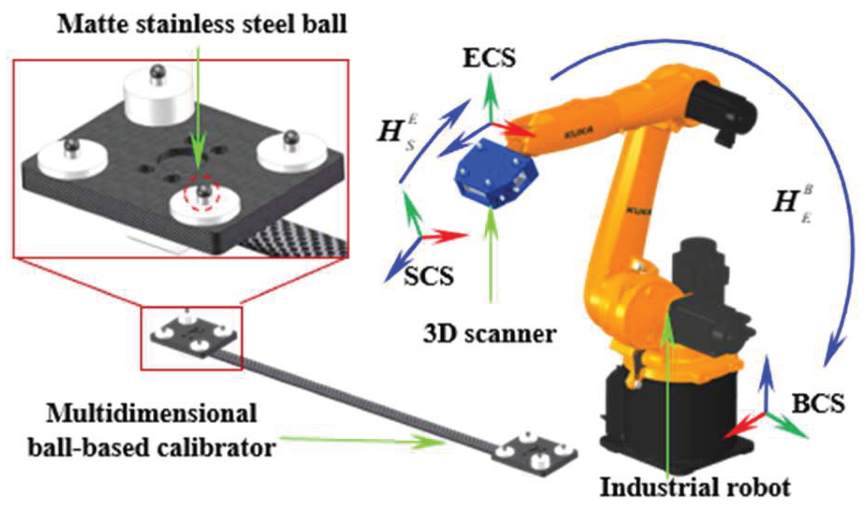
Figure 2.
Diagram of the single virtual point.
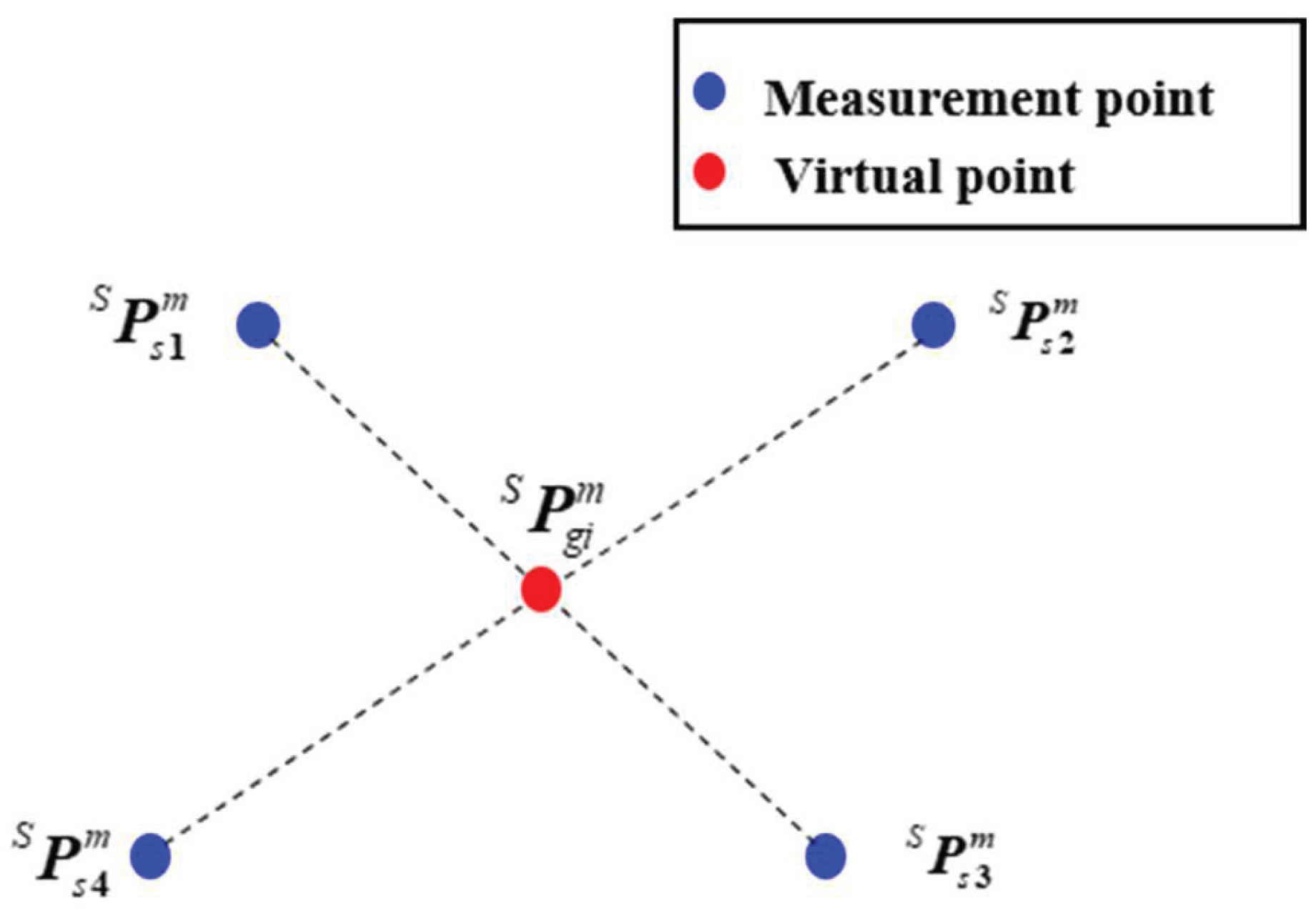
Figure 3.
Diagram of the spatial angle.
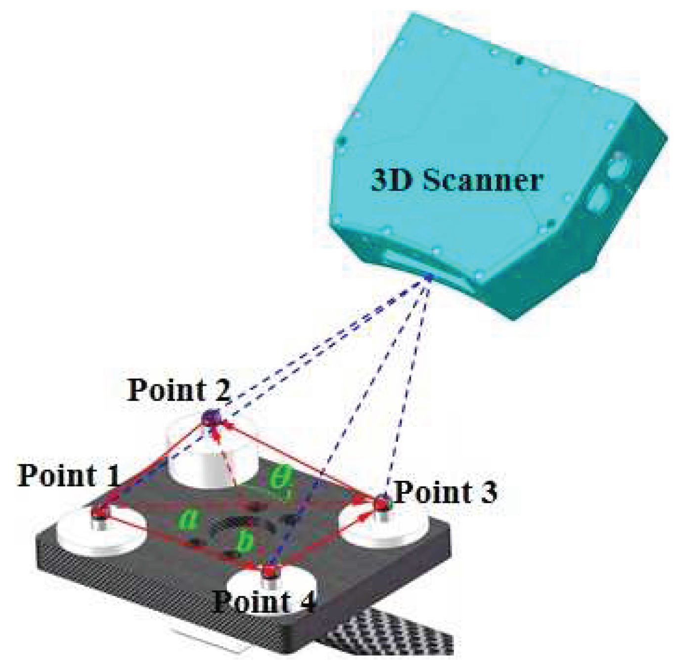
Figure 4.
Schematic of distance error.
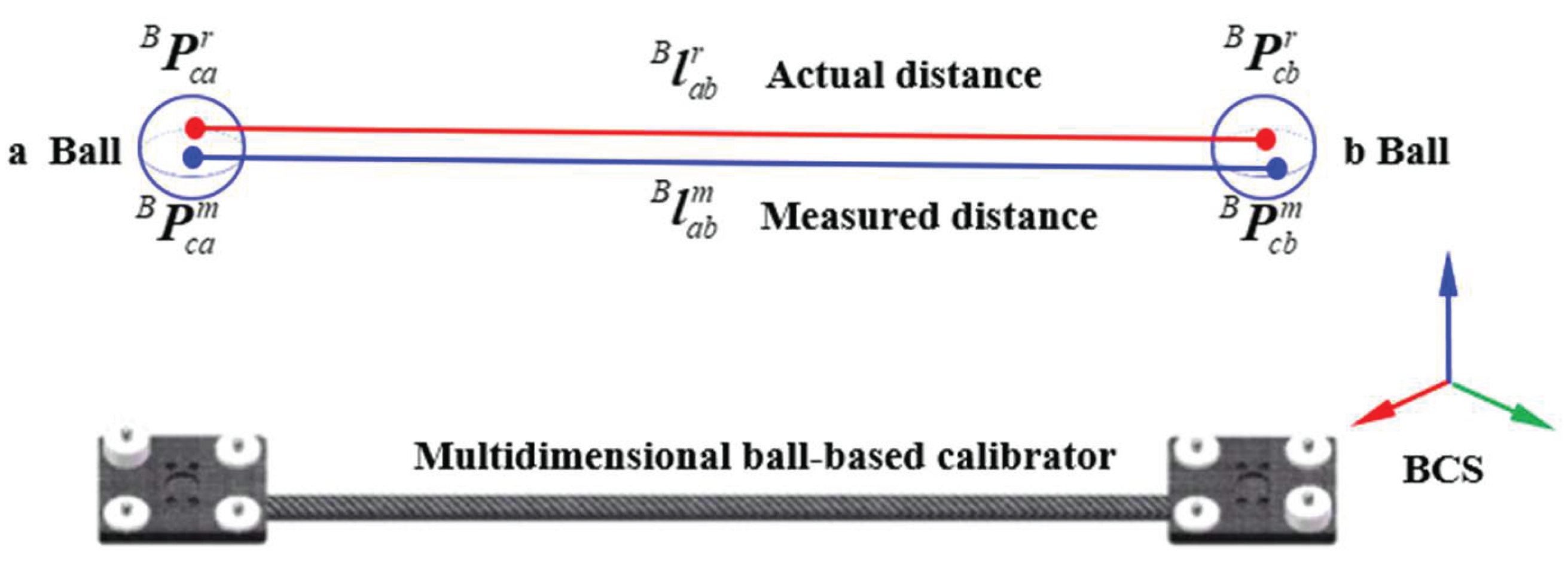
Figure 5.
Proposed flexible 3D scanning system.
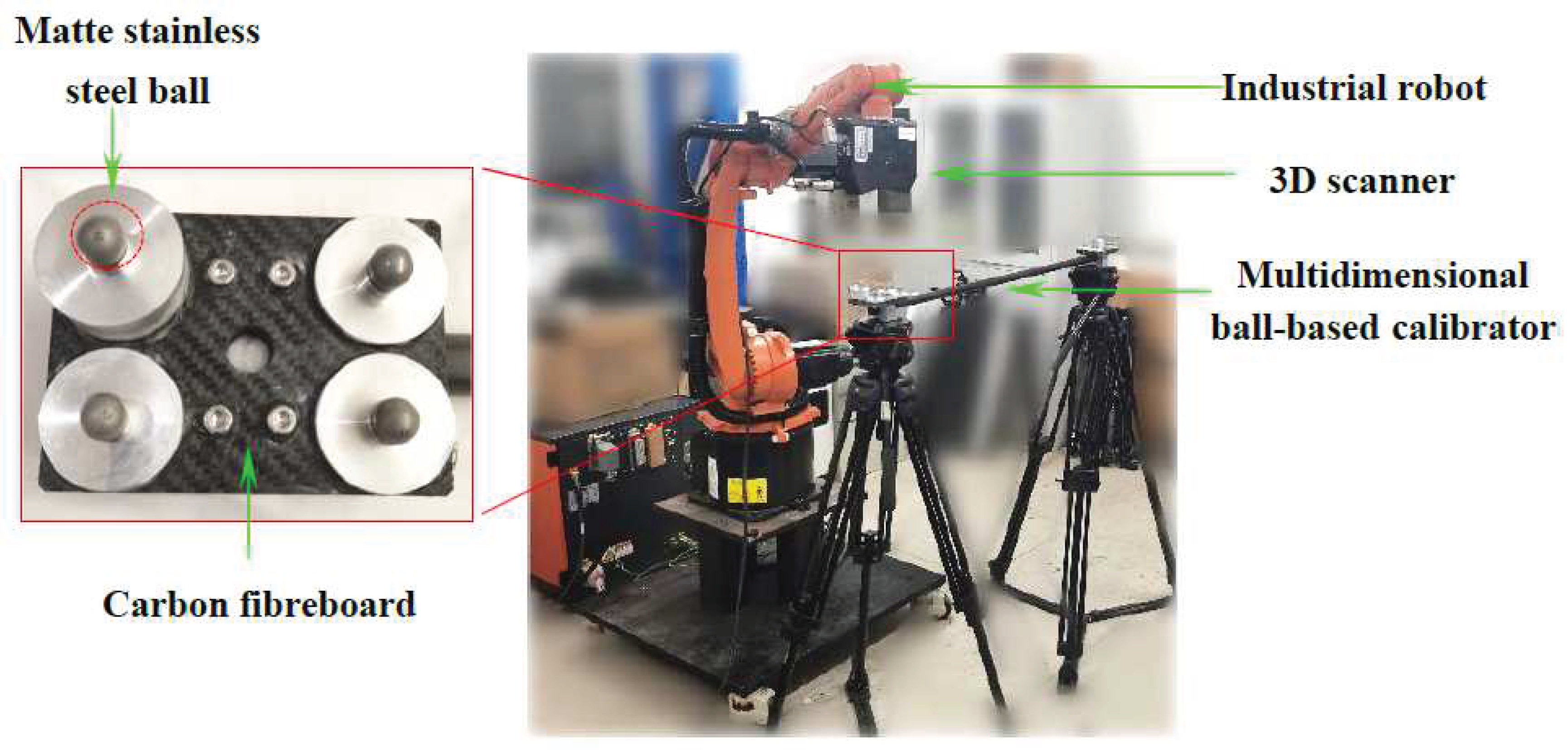
Figure 6.
Standard scale used for accuracy verification.
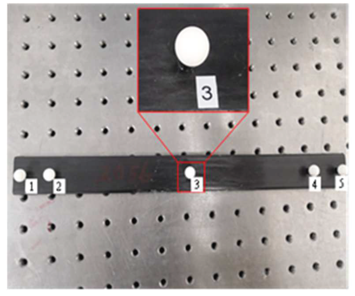

Table 1.
Identification results of robot parameter errors.
| Link No. | /° | /mm | /mm | /° | |
|---|---|---|---|---|---|
| 1 | 0.021 | 0.454 | 0.143 | 0.007 | — |
| 2 | −0.017 | — | −0.261 | 0.002 | 0.008 |
| 3 | 0.031 | −0.217 | 0.051 | −0.013 | — |
| 4 | −0.041 | 0.067 | 0.0268 | 0.001 | — |
| 5 | 0.027 | −0.081 | −0.002 | −0.014 | — |
| 6 | −0.024 | 0.102 | 0.036 | 0.021 | — |
Table 2.
Sphere spacing errors before and after calibration (unit: mm).
| No. | 1 | 2 | 3 | 4 | 5 | MPE | ME |
|---|---|---|---|---|---|---|---|
| Before | 0.721 | 0.837 | 1.041 | 0.712 | 0.734 | 1.041 | 0.809 |
| After | 0.457 | 0.347 | 0.428 | 0.375 | 0.364 | 0.428 | 0.394 |
Disclaimer/Publisher’s Note: The statements, opinions and data contained in all publications are solely those of the individual author(s) and contributor(s) and not of MDPI and/or the editor(s). MDPI and/or the editor(s) disclaim responsibility for any injury to people or property resulting from any ideas, methods, instructions or products referred to in the content. |
© 2025 by the authors. Licensee MDPI, Basel, Switzerland. This article is an open access article distributed under the terms and conditions of the Creative Commons Attribution (CC BY) license (http://creativecommons.org/licenses/by/4.0/).
Copyright: This open access article is published under a Creative Commons CC BY 4.0 license, which permit the free download, distribution, and reuse, provided that the author and preprint are cited in any reuse.


