
Submitted:
22 June 2025
Posted:
23 June 2025
You are already at the latest version
Abstract
Many publications have been devoted to the problem of parametric identifiability (PI). The major focus is on a priori identifiability. The parametric identifiability problem using experimental data (the so‐called practical identifiability (PID)) is less studied. This is a parametric identification task. PI has not been studied using current data (in adaptive systems). We propose an approach to estimating PI based on the application of Lyapunov functions. The role of the excitation constancy is shown. Conditions of local parametric identifiability (LPI) for a class of linear dynamical systems are got based on current experimental data. The case is considered when both the state vector and the input‐output set are measured. Estimates are obtained for the parametric residual. Case of limiting LPI on the set of current data is studied. Influence of initial conditions on PI is analysed. The case of m‐parametric identifiability is studied. Approach to estimating the PI of linear dynamical systems and systems with periodic coefficients based on the application of Lyapunov exponents is proposed. The LPI of decentralised systems is analysed. Examples are given.
Keywords:
parametric identifiability
; periodic dynamical system
; Lyapunov function
; adaptive algorithm
; decentralized system
; nonlinearity
; quadratic condition
; Lyapunov exponent
1. Introduction
Estimation of the model parameters is possible if the conditions guaranteeing their receipt are met. Many publications have been devoted to the issues of identifiability (see, for example, [1,2,3,4,5,6,7,8,9,10]). Much attention is paid to the analysis of a priori identifiability (AI) (in the literature, it is structural identifiability). AI conditions often have an algebraic form. To obtain them, such approaches are used as differential algebra [11], time series analysis [12] and some others [4,13,14,15]. The observability role [16] in identifiability problems is noted.
Some authors study the identifiability problem based on experimental data (see review [4]). This is practical identifiability. PID is based on obtaining a mathematical model and verifying it. This approach gives good results for systems with a known structure. In [17], low-order models are used to solve the problem of unidentifiable parameters. This approach is based on performing many adjustments.
Statistical hypotheses and criteria are used to solve the problem of estimating unidentifiable parameters. The probability profile parameter is used in [18]. Markov chains based on the Monte Carlo method [19] are used to estimate unidentifiable parameters. The apply of these approaches is associated with certain difficulties.
The Fisher information matrix is used to solve of PID problems [20]. Other statistical approaches are discussed in [4]. The result of solving the PID problem is the model with an accurate forecast. If this is not true, then the structural identification problem is solved. A more complete analysis of the state of the PID problem is given in the review [4]. Note that the PID problem interpretation does not accurately reflect the problem. This is the parametric identification problem with decision-making elements.
As follows from the presented analysis, the emphasis is on the study AI problem. Practical identifiability has not been sufficiently investigated. The focus is on synthesizing a mathematical model using various methods and evaluating its predictive properties. Various statistics, methods, and criteria are used to decision-making about the PRI. If the parametric identifiability condition is not met, various multistep procedures are proposed. These approaches are not always effective. For a more complex class of systems (multidimensional, decentralized, and interconnected), this problem requires further investigation. PI issues were not considered in adaptive systems.
In this paper, we study the PI problem for a class of adaptive models. The approach is proposed for obtaining conditions of local PI based on a class of adaptive algorithms. Conditions for limiting LPI are obtained. We show the dependence of adaptive identification system (ASI) properties on the initial conditions. A generalization of the results is given for the case of m-parametric identifiability. The linear system case with periodic parameters is considered. The PI problem solution is reduced to the application of Lyapunov exponents.
2. Problem Statement
Consider the system
where , are input and output, is the state vector, , , .
Set of experimental data
Assumption 1.
is Hurwitz matrix.
Problem. Evaluate the system (1) parametric identifiability using the of the set analysis.
3. Approach to PI Estimation
The representation is valid for the system (1) in space
:
where is the vector of parameters, is the generalised input vector, which is got based on the processing by a system of auxiliary filters.
To evaluate elements of vector , introduce the model based on the set for each :
where is the vector of model parameters, is the parameter setting the properties of the model.
Equation for identification error (prediction)
:
where .
Let the elements of the vector
by constantly excited (CE):
where .
Notation:
(i)
is a class of systems (1);
(ii) is a congruent representation (4) on the set ;
(iii)
is the frequency spectrum of the element
;
(iv)
or
;
(v)
if the CE condition is not held true.
(vi) the variable is if it has a non-degenerate frequency spectrum for all .
Definition 1.
The system (1) of class is locally parametrically identifiable on the set if the condition
is fulfilled for its representation (4) in class , where is some reference vector of system parameters (4), .
We see if there is an identification algorithm vector of the system (5) on for some , then starting from the moment , the condition (8) will be fulfilled for the estimates of vector .
Consider the Lyapunov function .
Theorem 1.
Let 1) assumption 1 holds, i.e., the matrix in (1) ; 2) the system (1) represents how (4) to set ; 3) the identification system is described by equation (6); 4) ; ,. Then the system (4) is locally parametrically identifiable in the region if follows from and the condition is satisfied:
where
,
is the unit matrix.
The proof of Theorem 1 is given in Appendix A.
Remark 1.
The vector reconstruction in (1), based on (4) and schemes proposed in the literature, gives estimates that do not correspond to components . This follows directly from (4). Therefore, adaptive control laws based on the use of vector elements are applied in control systems. Estimation , can be obtained directly from (4). The remaining components are determined based on the symbolic differentiation operation.
Corollary from Theorem 1.
If the adaptive algorithm
is used to evaluate the vector A in (4), then the local parametric identifiability of the system (1) follows from the estimation
where
,, is a diagonal matrix.
Let vector elements be measurable for each . Here, the system (4) is detectable. Then observability, detectability and recoverability of the system (1) follow from properties of system (4).
The proof corollary from Theorem 1 is given in Appendix B.
Consider the Lyapunov (LF) function , where .
Structures of classes and are congruent, so the following statement is valid for system (1).
Theorem 2.
Let 1) the conditions of Theorem 1 are fulfilled for the system (4) of class ; 2) classes and are congruent; 3) , . Then system (1) is locally parametrically identifiable on class if
where, , , , , is the matrix trace.
The proof of Theorem 2 is given in Appendix C.
Consider the adaptive model
and apply the integral algorithm class
to tuning of matrix .
The identification system is described by the equation:
where , is model (11) state vector, is the matrix of dimension .
Corollary from Theorem 2.
If the conditions of Theorem 2 are fulfilled, and the class of algorithms (12) is used to tuning the model (11) parameters, then the local parametric identifiability of the system (1) follows from the estimation
The proof corollary from Theorem 1 is given in Appendix D.
We see that the local PI depends on the choice of initial conditions, and fulfilment of the requirements for variables and system input.
Remark 2.
Presented results differ from the results [4] based on the application of AI methods. If the decision is made based on experimental data, then various statistics [4] are used. In this paper, we apply the approach to the PI analysis based on the current data analysis. This approach has not been used in PI tasks.
If conditions of Theorem 2 are fulfilled, then the class of algorithms (12) will be called locally identifying.
In the future, for the convenience of reference, the adaptive algorithm (10) will be related to class , and the law (12) to class .
Definition 2.
A system (1) of class is extremely locally parametrically identifiable (ELPI) on the set if the condition
is satisfied for its representation (4) in class , where is some reference vector of system (5) parameters, , is an area of zero.
Here, the vector identifiability is understood as the limit proximity to . Under certain conditions, the global PI of the vector follows from (15).
Consider again the system (6) and LF .
Theorem 3.
Let the conditions of Theorem 1 be fulfilled and (i) there is a Lyapunov function admitting an infinitesimal upper limit; (ii) there is such that the condition is satisfied for sufficiently large in some area of zero; (iii) with parameters ; (iv) The inequality
is valid for the trajectories of the adaptive system (6) and (10), where is the minimum eigenvalue of the matrix . Then the system (6), (10) is locally parametrically identifiable on the set with estimating if the functional condition
is satisfied, where:
is the upper solution of the comparison system for (16) if , , .
The proof of Theorem 3 is given in Appendix E.
We see that the PI in the class of algorithms (10) or (12) depends on the initial conditions and properties of the information set. LPI is guaranteed for systems of class and with asymptotic stability by error. However, estimate elements of the matrices will belong to the domain . This is a typical state of adaptive identification systems based on the class of algorithms (10), (12).
Remark 3.
The region can be compressed to and limiting conditions for LPI can be got if conditions (9) or (17) for ASI are fulfilled. In real-world conditions, ASI guarantees almost extremely local parametric identifiability.
4. On ELPI
The ELPI fulfilment guarantees the transition to global PI (GPI). For static procedures (least squares method, maximum likelihood method), ELPI is ensured by the properties of the information matrix. For methods based on the class , properties of the information matrix are not directly applicable, because the processes are complex in ASI.
With GPI, we understand the condition fulfilment:
The proposed interpretation of GPI as belonging the parameters of model (6) to the set is linked to the absolute stability of an adaptive system.
Global parametric identifiability follows from Theorem 4 for systems of class .
Theorem 4.
Let: 1) the conditions of Theorems 1 and 3 are fulfilled; 2) The system of inequalities is valid for processes in the system (6), (10)
where are the maximum and minimum eigenvalues of the matrix . Then (a) the system (4) is globally parametrically identifiable on the class , (b) the system (6), (10) is exponentially stable with the estimate:
if
where is the state vector of the comparison system , .
The proof of Theorem 4 is given in Appendix F.
From Theorem 4, we obtain GPI on the set of initial conditions and ELPI. Since the systems are congruent, this condition is also valid for systems (1) of class . To substantiate this statement, apply the approach [22].
5. About m-Parametric Identifiability
Let the CE condition not be fulfilled. The problem of identifiability, and identification, must be solved. Consider the approach to solving this problem using the example of the class system.
Let the system and the model have the form (4) and (5). We assume that . The term in (6) is represented as
where ; is the representation corresponding to the vector .
Transform the equation for error (6) to the form
where , is uncertainty caused by non-fulfilment of the condition , , is the part of the vector evaluated on the class , , .
Let , where .
Definition 3.
A system of class is -locally parametrically identifiable on the set if the condition
is satisfied with its representation (4) in class .
Theorem 5.
Let (i) the system (1) be stable; (ii) the Lyapunov function admits an infinitesimal limit, where is the diagonal matrix; (iii) . Then the system (4) is locally parametrically identifiable in the domain if
and all trajectories of the system (4) belong the area
where , .
The proof of Theorem 5 is given in Appendix G.
From Theorem 5, we see that the PI domain depends on the CE fulfilment of the information set of the system. If the CE condition is not fulfilled, the parameter increases because of the effect of parametric uncertainty . Here, estimate (14) is more realistic and, under certain conditions, ELPI is possible with estimate (18).
Remark 4.
In biological systems, structural identifiability issues are considered. Most times, lineal systems with numerous parameters are studied. Various algorithms are proposed and identifiability conditions are investigated to reduce the number of estimated parameters. In ASI, a multiplicative approach is used to identify a system with various parameters [23]. Here, PI is understood as parametric identifiability in some parametric domain , depending on the vector of multiplicative parameters (MPV). As a rule, MPV estimates belong to a certain limited area, which is formed based on of a priori information and analysis of the information set. This identifiability applies to systems satisfying specified quality requirements.
6. Lyapunov Exponents in PI Problem
6.1. Stationary System of Class
Lyapunov characteristic exponents (LE) are the characteristic of a dynamical system. LE is an indirect PI estimate of the system. This approach to PI has not been considered in the literature. The LE application has its own peculiarities in the proposed paradigm of PI. In particular, it is necessary to consider the issue of detectability, recoverability and identifiability of LE based on the information set of the system. Identifiability is understood as the detectability of Lyapunov exponents. Known approaches allow us to estimate only the maximum (largest) LE [24]. A more promising approach is based on the analysis of geometric frameworks (GF) reflecting the change in LE [24]. Issues of LE detectability based on GF analysis are presented in [24]. Therefore, they are not considered here. Detectability is the important issue for evaluating LE.
In [24], the criteria for -detectability of Lyapunov exponents are presented. -detectability and recoverability we understood as the ability to the LE estimate. -detectability imposes certain requirements on experimental data. The approach allows us to obtain the full range LE.
Let , where is the number of non-recoverable LE.
Definition 4.
The system (1) is called -detectable with a -non-recoverability level if the lineal (LE) has an insignificant level.
As follows from definition 4, that if the system of class is -detectable with a level of -non-recoverability, then this is a sufficient condition for -parametric identifiability of the system. The CE requirement plays an important role, as it guarantees the S-synchronizability and structural identifiability of the nonlinear system.
Remark 5.
The definition 4 provides sufficient conditions for evaluating PI systems of class . This issue requires further study. Note that LE (for the classes under consideration, the Lyapunov exponents are the eigenvalues of the matrix) depend on system parameters.
Analysing nonstationary (periodic) systems is more difficult, since it is difficult to isolate the parametric space here.
Using LE translates the PI problem into the space of Lyapunov exponent [25] for periodic systems (PS).
6.2. PS for Class
Consider the system (1) with the matrix . For convenience, the system will be denoted by .
Assumptions.
A1. is a bounded continuous Frobenius matrix
where , is matrix norm.
A2. is almost periodic, i.e., a subsequence can be selected from any sequence
converging uniformly along the entire axis to some almost periodic matrix .
A3. is the Hurwitz matrix for almost all
Let is a spectrum of LE .
Definition 5.
The function is almost periodic in the Bohr sense [26] or the - function [25], if such a positive number exists, that any segment contains at least one number , for which it is hold
If is a -function, then it is -almost periodic [26], where are positive numbers.
Let the order of the system be known. Apply the geometric structure to decide on the spectrum [26]. Here , , is an evaluation of the general solution of the system (1).
described by the function , where . is -function, contains areas , where a drastic change is taking place.
Theorem 6.
If the system is stable and recoverable, and the function contains at the interval at least regions , then the system has an order and is -identifiable (-detectable).
In terms of Theorem 6, is a time interval in which an estimate of the general solution of the system are obtained.
It follows from Theorem 6 that the system is identifiable on the set . As shown in [25], the location of local minima on coincides with regions of the structure . This result allows us to obtain the set containing estimates LE of the system . Cardinal may not match the LE number of the system. characterizes the set of system lineals.
The detectability (identifiability) of the periodic system (1) with the matrix follows from [25].
Theorem 7.
Let 1) assumptions A1-A3 are fulfilled for the system; 2) the system is recoverable; 3) ; 4) set elements are -functions; 5) the structure contains at least regions of , which to local minima correspond to the structure . Then the set is -detectable or fully detectable.
Corollary from Theorem 7.
If structures contain only of regions , which to local minima correspond on , then the system is -detectable with an -non-recoverable level.
Remark 6.
Eigenvalues of the matrix are periodic functions of time. Therefore, lineals and corresponding to these functions may overlap. This can generate an infinite range of LE. Determine the acceptable range for and the number that determines the mobility of the largest Lyapunov exponent. The set upper bound is determined by the allowable mobility limit of the largest LE . The estimate is fair for [25]:
where is the interval of the change of the ith indicator . The region lower boundary is bounded by the smallest LE [25].
Definition 6.
The system of class with matrix satisfying assumptions A1–A3 is locally -identifiable on the set , if spectrum of LE belonging to the class -function exists such that
where .
The problem of assessing the LE adequacy has its own specifics. Let is phase portrait of the system .
Definition 7 [25].
Estimates of Lyapunov exponents are -adequate in the space, if areas of their definition coincide with -almost-periodicity regions of structure .
Theorem 8 [25].
Let:(i) the -system is stable and recoverable; (ii) the set is -detectable; (iii) definition regions on the structure coincide with -almost-periodicity regions for the G5 structure . Then estimates of elements for the set are -adequate to the regions -almost periodicity .
Remark 8.
We have considered only one approach to assessing the PI of periodic systems. The PS can be considered as a system with an interval parametric domain and identifiability can be estimated within the specified limits. Here, the approaches described above in Section 4 and Section 5 are applied.
So, the problem of estimating LPI is reduced to a more adequate task of estimating LE for these systems. The PI conditions in a special space are got and the methods of its estimation are given. The adequacy concept of LE estimates is introduced and the area for the LE location is highlighted. We have shown the existence of a LE set for the system .
7. About LPI for Decentralized Systems
Consider a decentralized system (DS)
where , are state and output vectors of the -subsystem, is control, , . The elements of the matrices are unknown; . The matrix reflects the mutual influence of the subsystem . considers the nonlinear state of subsystem 2, and the is the Hurwitz matrix (stable).
Assumption 2.
belongs to the class
and satisfies the quadratic condition
where .
The information set of measurements for the -subsystem has the form
Mathematical model
where is a matrix with known elements; , are tuning matrices, is a priori defined nonlinear vector function.
Problem. Obtain PI estimates for the system (32) based on the set analysis.
DS (32) is nonlinear, so the condition CE (7) is represented as:
Where is the set of frequencies for ; is the set of acceptable frequencies of input , ensuring S-synchronizability of the system.
Get the equation for the error :
where are parametric residuals.
Consider the system (37) and LF , where is a positive symmetric matrix.
Let , are the norm of matrixes , , is the trace of the matrix.
The following modification of Theorem 1 [27] is true.
Theorem 9.
Let: 1) the matrix ; 2) , ; 3) and
where , , , , . Then subsystem (32) is locally parametrically identifiable on the set if
where , is the minimum eigenvalue of the matrix ; , , .
The proof of Theorem 9 is given in Appendix H.
Corollary 1 of Theorem 9.
Let conditions of Theorem 9 be fulfilled. Then the nonlinearity is locally structurally identifiable in the parametric sector
if
where .
The proof corollary 1 from Theorem 9 is given in Appendix I.
Consider the system (37) and class algorithms to tune its parameters:
where , , are diagonal matrices of the corresponding dimensions.
Lyapunov function for analysis of system (37) and (4): :
Corollary 2 of Theorem 9.
Let 1) conditions of Theorem 9 be fulfilled; 2) the class of algorithms is used to tuning parameters of the model (35). Then the system (32) is locally parametrically identifiable if
where , ; are The minimum and maximum eigenvalues of the matrix , and the estimate is held
The proof corollary 2 from Theorem 9 is given in Appendix J.
As follows from Theorem 9, system (32) is LPI and structurally identifiable with nonlinearity in the parametric sector on the set of initial conditions and .
If we perform nonlinearity factorization (see, for example, [27])
where is a priori estimation of known parameters, is vector of tuning parameters, the structure is formed a priori considering the known vector , and apply the algorithm
where is a diagonal matrix with positive diagonal elements, then we obtain the conditions for global parametric identifiability for DS on the class of algorithms and (44). They are based on the modernization of results [27].
8. Examples
1. Consider an engine control system with the Bouc–Wen hysteresis
where is mass, is damp, is the recovering force, , , , , is exciting force, are some numbers. Set of experimental data . Vector of parameters .
Model for system identification (48)
where ; , , are adjustable model parameters. Let . From (48) and (49), we obtain the equation for the identification error:
where , .
The variable is not measured. Apply the model to estimate :
and introduce a residual . Let is current estimate . Then we get the model to evaluate
where ; , are estimates of hysteresis parameters (47); , is the integration step.
Introduce a residual , satisfying equations
where , , . Present (49) as:
and (50) is written as:
Evaluate the identification quality using the Lyapunov function. . Get adaptive algorithms from :
where are parameters ensuring the stability of algorithms (57).
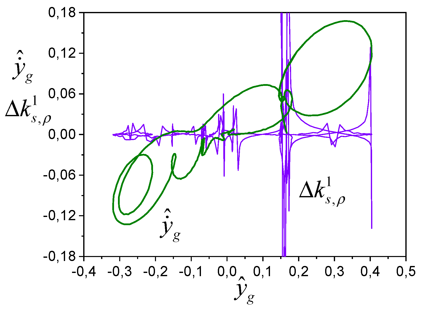
Consider functionals:
Figure 1 and Figure 2 represent PI evaluations of the system (45) – (47). The ASI has two loops: the main one (variable ) and the auxiliary one (variable ). Figure 1 shows the structure described by the function , and Figure 2 presents the structure described by the function .
Presented structures confirm the fulfilment of the Theorem 1 conditions, since trajectories of the system for sufficiently large get into the region .
2. Consider the system, the phase portrait of which is shown in Figure 3. The set of experimental data is known. Input . Figure 3 shows the presence of oscillations in the system, the frequency of which differs from the frequency of the input. Therefore, the system is the system with periodic coefficients.
To determine LE, we apply the approach [25] and obtain estimates of the general solution and its derivative.
The coefficients of determination for these models are equal 0.99. Next, we determine estimates of the free movement for the system. The evaluation of order for the system follows from Figure 4.
It follows from that the system has a third order. From and , we get the set LE (Figure 4).
The upper estimate for is . Mobility limit for is –0.8. -adequacy confirmation of LE estimates is shown in Figure 5. The eigenvalues of the state matrix of the system are:
So, we see that the set is -detectable, and the system has the third order. Since the elements of the set are recoverable and detectable, the system is LPI.
9. Conclusion
The problem of estimating parametric identifiability based on current experimental data is considered. Methods of the priori identifiability based on the analysis of the information matrix are not applicable in this case. We consider the approach based on the application of the second Lyapunov method to the PI study. LPI conditions are got based on the adaptive identification application to the linear dynamical system. We analyse data on state vector and current information on input and output in the problem PI. Conditions and estimates have been obtained that guarantee PI and LPI.
The -parametric identifiability case is considered when the condition of constant excitation is not fulfilled. PI estimates are got for decentralised nonlinear systems and systems with periodic parameters. We show that Lyapunov exponents should be used to PI analyses of the system with periodic parameters.
Modelling examples are presented that confirm the efficiency of the proposed approach.
Appendix A
Proof of Theorem 1.
Consider the LF . For , we get:
or, applying condition 4 of Theorem 1,
where , .
Let and correspond to Fourier series with multiple frequencies , where depends on the spectrum . System (1) is a frequency filter and . Therefore, the frequency spectra of the elements of the vector will vary. Therefore, sets , where , will not have common areas. Then follows from the identifiability condition .
So, condition 4 is necessary for the local identifiability of the system (6). As condition 4 is fulfilled, for the limited trajectories (identifiability) of the system (4), it is necessary that:
Appendix B
Proof of Corollary 1 from Theorem 1.
For , we get:
where , . Let . Present (B.1) as:
where from
or .■
Appendix C
Proof of Theorem 2. The derivative LF has the form
or
where , , is a positive definite matrix satisfying the equation , . Then (C.2)
where , , , is the identity matrix.
From (C.3), we obtain the condition of LPI:
Appendix D
Proof of Corollary 1 from Theorem 2.
Consider LF , where:
are diagonal matrices with positive diagonal elements.
If we consider (12), then (C.1) is written as:
Obtain
Appendix E
Proof of Theorem 3. Apply algorithm (10) and represent the derivative as:
Let exist such that in some region 0 the condition is satisfied.
Then (E.1)
As и , then
Apply the inequality [29]
Then
As , where is the minimum eigenvalue of the matrix . Then:
It follows from (E.5) that PI is guaranteed on a certain set and on the set if
and fair evaluation , where:
, is the upper solution of the comparison system for (E.5), if ,.■
Appendix F
Proof of Theorem 4. From the proofs of the corollary of Theorem 1 and Theorem 3, we obtain
As , then (F.1)
The matrix is an -matrix [30] if conditions are fulfilled for the major minors. Obtain
If the conditions (F.3) are fulfilled, then the adaptive system (6), (10) is exponentially stable (ES). As follows from the ES, estimates of the vector in (4) are extremely locally parametrically identifiable under given initial conditions. The estimate (21) is got using the approach described in the proof of Theorem 3.■
Appendix G
Proof of Theorem 5.
Consider (23) and represent the derivative of LF as:
or
where , . From (G.2), we obtain the condition -local PI:
Represent (G.1) in the form
Then (G.4)
Transform (G.5)
Let , and . Then:
The estimate for (see (26)) follows from (G.7). ■
Appendix H
Proof of Theorem 9.
has the form:
or
where is the minimum eigenvalue of the matrix .
Apply the Cauchy-Bunyakovsky-Schwarz inequality and Titu’s lemma to the last term in (H.2) and get
Consider condition 1) of Theorems 9 and write as:
where . Apply Lemmas 1, 2 [26] and get for
where , , , .
Then (H.4)
If state variables are CE and the condition (38) is fulfilled, then the system (32) is the LPI on the set .■
Appendix I
Proof of Corollary 1 from Theorem 9.
As follows from Theorem 9, DS is locally parametrically identifiable if the condition (38) is satisfied. Apply Lemmas 1, 2 [26] to the last terms in (H.6) and get:
Therefore,
where .
As , then . ■
Appendix J
Proof of Corollary 2 from Theorem 9.
Represent (H.2) as:
Let , where . Then:
where are minimum and maximum eigenvalues of the matrix .
The estimate (H.5) is fair for . Therefore, (J.2) is represented as:
where . Let . Transform (J.3):
Then
if .■
References
- Villaverde A. F. Observability and structural identifiability of nonlinear biological systems. arXiv:1812.04525v1 [q-bio.QM] 11 Dec 2018, 2022. [CrossRef]
- Renardy M., Kirschner D., and Eisenberg M. Structural identifiability analysis of age-structured PDE epidemic models. Journal of Mathematical Biology, 2022, 84(1-2); 2022. [CrossRef]
- Weerts, H. H. M., Dankers, A. G., &, Van den Hof, P. M. J. Identifiability in dynamic network identification. IFAC-PapersOnLine, 2015, 48(28), pp. 1409-1414. [CrossRef]
- Wieland F.-G., Hauber A. L., Rosenblatt M., Tönsing C. and Timmer J. On structural and practical identifiability. Current opinion in systems biology, 2021, 2, pp. 60–69. [CrossRef]
- Miao H., Xia X., Perelson A. S., and Wu H. On identifiability of nonlinear ode models and applications in viral dynamics. SIAM Rev Soc Ind Appl Math, 2011; 53(1), pp. 3–39. [CrossRef]
- Bellman R, Åström K: On structural identifiability. Math Biosci. 1970, 7, pp. 329–339. [CrossRef]
- Anstett-Collina F., Denis-Vidalc L., Millérioux G. A priori identifiability: An overview on definitions and approaches. Annual reviews in control, 2021, 50, pp.139-149. [CrossRef]
- Hong H., Ovchinnikov A., Pogudin G., Yap C. Global identifiability of differential models. Communications on Pure and Applied Mathematics, 2020, 73 (9). 18311879. [CrossRef]
- Denis-Vidal L., Joly-Blanchard G., Noiret C., System identifiability (symbolic computation) and parameter estimation (numerical computation). Numerical Algorithms, 2003, 34(2-4), pp. 283–292. [CrossRef]
- Boubaker O., Fourati A., Structural identifiability of nonlinear systems: an overview. In: Proc. of the IEEE International Conference on Industrial Technology, ICIT’04, December 8-10, 2004, pp. 1244–1248. [CrossRef]
- S. Audoly, G. Bellu, L. D’Angi `o, M. P. Saccomani, and C. Cobelli. Global identifiability of nonlinear models of biological systems. IEEE Trans. Biomed. Eng., 2001, 48(1), pp. 55–65. [CrossRef]
- Chis O.-T., Banga J. R., and Balsa-Canto E. GenSSI: a software toolbox for structural identifiability analysis of biological models. Bioinformatics, 2011, 27(18), pp. 2610–2611. [CrossRef]
- Denis-Vidal L., Joly-Blanchard G., and Noiret C. Some effective approaches to check the identifiability of uncontrolled nonlinear systems. Math. Comput. Simul, 2001, 57(1), pp. 35–44. [CrossRef]
- X. Xia and C. H. Moog. Identifiability of nonlinear systems with application to HIV/AIDS models. IEEE Trans. Autom. Control, 2003, 48(2), pp. 330–336. [CrossRef]
- Stigter J. D. and Molenaar J. A fast algorithm to assess local structural identifiability. Automatica, 2015, 58, pp. 118–124. [CrossRef]
- Villaverde A. F. Observability and structural identifiability of nonlinear biological systems. Complexity, 2019, Article ID 8497093. [CrossRef]
- Hengl S., Kreutz C., Timmer J. and Maiwald T. Data-based identifiability analysis of non-linear dynamical models. Bioinformatics, 2007, 23(19), pp. 2612–2618. [CrossRef]
- Murphy S.A, van der Vaart AW: On profile likelihood. Journal of the American Statistical Association, 2000, 95, pp. 449-465. [CrossRef]
- Raue A, Kreutz C, Theis F.J., Timmer J. Joining forces of Bayesian and frequentist methodology: a study for inference in the presence of non-identifiability. Phil Trans R Soc A, 2013, 371:20110544. [CrossRef]
- Neale MC, Miller MB: The use of likelihood-based confidence intervals in genetic models. Behav Genet, 1997, 27, pp. 113–120. [CrossRef]
- Cedersund G: Prediction uncertainty estimation despite unidentifiability: an overview of recent developments. In Uncertainty in biology, 2016, pp. 449–466. [CrossRef]
- Karabutov N. Identification of decentralized control systems. Preprints ID 143582. Preprints202412.1808.v1. [CrossRef]
- Karabutov N. Adaptive observers for linear time-varying dynamic objects with uncertainty estimation. International journal of intelligent systems and applications, 2017, 9(6), pp. 1-15. [CrossRef]
- Karabutov N.N. Identifiability and Detectability of Lyapunov Exponents for Linear Dynamical Systems. Mekhatronika, Avtomatizatsiya, Upravlenie, 2022, 23(7), pp. 339-350. [CrossRef]
- Karabutov N. Identifiability and detectability of Lyapunov exponents in robotics. In Design and control advances in robotics, Ed. Mohamed Arezki Mellal, IGI Global Scientific Publishing, 2022, 10(11), pp. 152-174. [CrossRef]
- Bohr G. Almost periodic functions. Moscow: Librocom, 2009.
- Karabutov N. Adaptive identification of decentralized systems. In Advances in mathematics research. Volume 37. Ed. A. R. Baswell. New York: Nova Science Publishers, Inc. 2025. 79-115.
- Karabutov N.N., Shmyrin A.M. Application of adaptive observers for system identification with Bouc-Wen hysteresis. Bulletin of the Voronezh State Technical University, 2019, 15(6), pp. 7-13.
- Barbashin E. A. Lyapunov functions. Moscow: Nauka Publ., 1970.
- Gantmakher F. R. Theory of matrices. Moscow, Nquka, 2010.
Figure 1.
Structure .
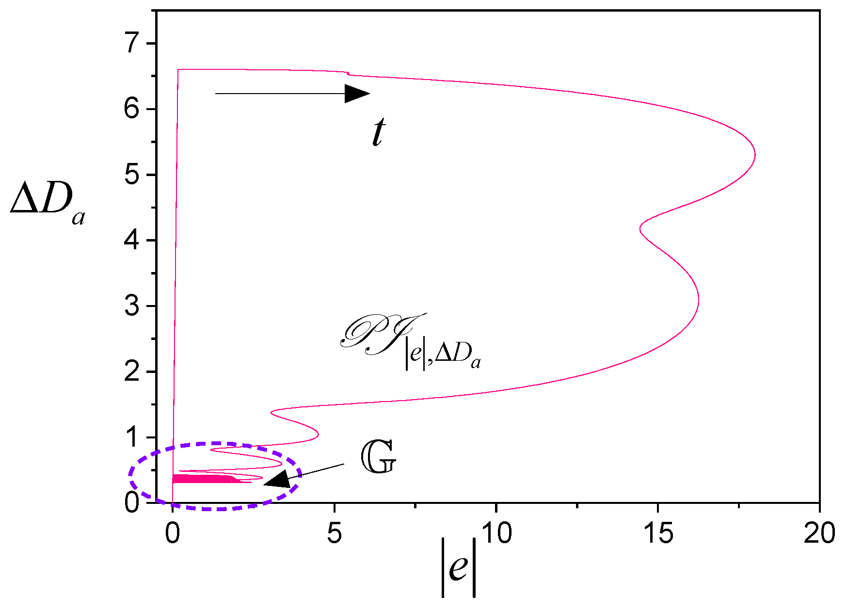
Figure 2.
Structure .
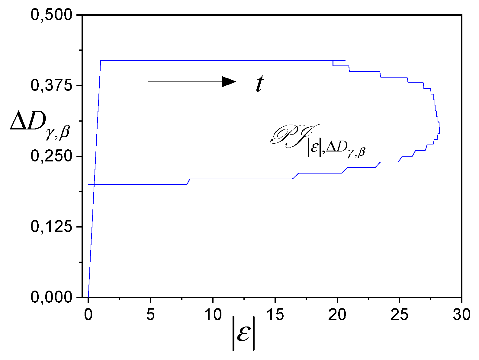
Figure 3.
Phase portrait.
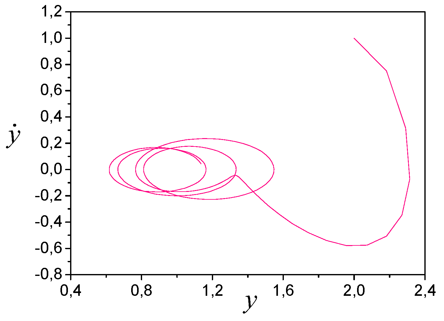
Figure 4.
LE set.
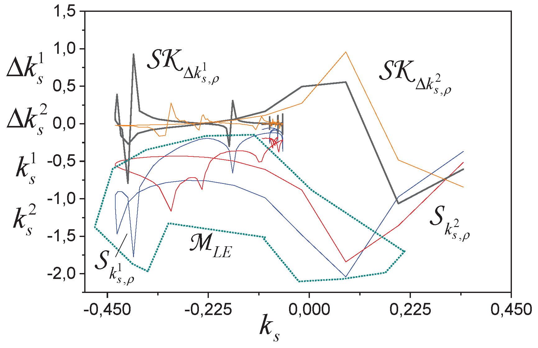
Figure 5.
Estimate of -adequacy of LE.
Disclaimer/Publisher’s Note: The statements, opinions and data contained in all publications are solely those of the individual author(s) and contributor(s) and not of MDPI and/or the editor(s). MDPI and/or the editor(s) disclaim responsibility for any injury to people or property resulting from any ideas, methods, instructions or products referred to in the content. |
© 2025 by the authors. Licensee MDPI, Basel, Switzerland. This article is an open access article distributed under the terms and conditions of the Creative Commons Attribution (CC BY) license (http://creativecommons.org/licenses/by/4.0/).
Copyright: This open access article is published under a Creative Commons CC BY 4.0 license, which permit the free download, distribution, and reuse, provided that the author and preprint are cited in any reuse.


