
Submitted:
18 June 2025
Posted:
19 June 2025
You are already at the latest version
Abstract
Bays are treasures of the coastal zone with highly concentrated wealth. As conflicts between protection and development intensify, bays have become focal areas for sustainable development research. As important carbon sinks with unique land use, assessing their carbon storage potential is highly significant. Human activities and climate change have increasingly impacted South China Sea Bay land use over 50 years. Carbon storage research based on remote sensing land use monitoring is crucial for environmental protection and low-carbon development. Using Johor Estuary Bay as a case, we employed multi-source remote sensing data and object-based segmentation for land use classification. A carbon storage response index was constructed to analyze land use changes and carbon storage impacts from 1977-2030. Results showed that: (1) Construction land expanded 10-fold while 76.29% of forestland was replaced by agricultural and residential land. (2) From 1977-2023, carbon storage showed a declining trend, with total reduction of 2.37×10⁵t. (3) Forestland and mangrove reduction contributed 65.50% and 13.33% to carbon loss respectively. (4) Ecological protection scenarios limiting construction land expansion while preserving forests and mangroves better maintain carbon storage. Therefore, future development should prioritize ecological protection and plan economic construction rationally on this foundation.
Keywords:
coastal zone
; remote sensing
; land use
; carbon storage
; South China Sea
1. Introduction
Carbon storage is a crucial component of the global carbon cycle and vital for mitigating global warming [1]. Against the backdrop of global climate change and rapid economic development, reducing carbon emissions alone is insufficient to address climate risks [2]. Enhancing the carbon storage capacity of ecosystems is imperative. Soil carbon pools in terrestrial ecosystems account for over 80% of global terrestrial carbon cycling [3]. Marine ecosystems also possess extremely high carbon fixation efficiency, with a per-unit carbon storage efficiency 15 times that of terrestrial systems [3]. The coastal zone serves as a link between land and sea, simultaneously encompassing both marine and terrestrial carbon pools [4]. It includes important marine ecosystems such as mangroves, tidal flats, and salt marshes, as well as terrestrial carbon reservoirs like forests and soils, all of which possess exceptional carbon storage capacity [5]. However, coastal zones experience significant population concentration [6], resulting in higher human disturbance and increased ecosystem vulnerability. Bays are the most geographically advantageous areas of the coastal zone, with highly concentrated resources and serving as main hubs for human development [7]. Significant location value, unique ecological environments, and frequent human activities make bays typical ecologically fragile and environmentally sensitive areas [8]. The conflict between protection and development is increasingly prominent, making bays a key focus of sustainability research [5]. Furthermore, bays are home to over 60% of the global population and are regarded as important transportation hubs or economic centers [9], thus facing greater pressure from carbon emissions.
Land use change profoundly affects soil structure and biological distribution, serving as a key driver of carbon storage variation [10]. Current research on carbon storage based on land use change can be divided into two main categories: biomass estimation [10,11] and modeling approaches [12,13]. Biomass estimation is time-consuming and less adaptable, making it difficult to accurately capture long-term carbon storage changes [10]. Thus, more recent studies tend to use modeling approaches, such as the Forestry and Carbon Cycle of China Model (FORCCHN) model [14], Multi-scale Comprehensive Assessment Tool - Denitrification-Decomposition (MCAT-DNDC) model [15], and Integrated Valuation of Ecosystem Services and Tradeoffs (InVEST) model [9]. Compared to InVEST, other models require more detailed data and numerous parameters, which increases their complexity and operational costs [16]. The InVEST model can estimate carbon storage more accurately and efficiently with fewer data and parameters, making it the most widely used [17]. For example, Babbar et al. used the InVEST model to assess carbon storage in the Sariska Tiger Reserve from 2000 to 2018 [18]. Bacani et al. predicted carbon storage in Brazil’s Cerrado eucalyptus production areas for 2030 under different scenarios using InVEST [19].
Common models for land use prediction include the Cellular Automata (CA) model [20], CA-Markov model [21], Future Land Use Simulation (FLUS) model [22], Conversion of Land Use and its Effects at Small regional extent (CLUE-S) model [23], and Patch-generating Land Use Simulation (PLUS) model [24]. CA and CA-Markov are discrete models that lack consideration of external influences and have low operational efficiency. The CLUE-S and FLUS models have limitations in structure and flexibility, making it difficult to handle complex land use scenarios [25]. The PLUS model, incorporating a Markov chain as well as CA and multi-objective programming (MOP), predicts land use patch evolution by analyzing driving factors of land change. It allows for more comprehensive simulation and prediction of land use change [26], leading to its widespread use. For example, Zhang et al. used the PLUS model to predict the landscape pattern of the Fujian Delta in 2050 [27], and Liang et al. explored the drivers of land expansion and landscape changes in Wuhan using the PLUS model [26].
The Johor Estuary is an important transportation hub for both Malaysia and Singapore [28]. Over the past 50 years, its population has grown rapidly from 2.1 million to 3.7 million—far exceeding the national growth rate of Malaysia (2.6%) [29]. This surge has driven up demand for food, housing, and other natural resources, resulting in significant changes in land use patterns and carbon storage. However, the frequent clouds and rain typical of South China Sea have limited the acquisition of remote sensing images and other geographic data [28], leading to relatively little research in the region. Advanced remote sensing technologies are therefore urgently needed as key research tools for coastal studies in this area. Additionally, previous studies on land use and carbon storage have largely relied on existing land use data and have lacked research into the response mechanisms of carbon storage to changes in land use types [12,30].
Here, our study aims to investigate the impact mechanisms of land use changes on carbon storage under multiple scenarios in bay areas, using the Johor River Estuary Bay in the South China Sea as a case study and leveraging multi-source remote sensing data. The specific objectives are: (1) To perform land classification through object-based segmentation with Gray Level Co-occurrence Matrix (GLCM) texture features and spectral indices. (2) To couple the InVEST-PLUS model to simulate and analyze land use changes in the Johor estuary from 1977-2023, and 2030 under three scenarios (natural development, ecological protection, and economic development). (3) To construct a Carbon Impact (CI) function to quantify the driving effect of each type of land use change on carbon storage. The findings will provide reference for low-carbon sustainable development and future land planning in the Johor estuary and other similar coastal regions.
2. Study Area and Data
2.1. Study Area
The Johor River Estuary Bay (1°20′–1°47′N, 103°50′–104°09′E) is located in the southern part of Johor State, Malaysia, and the eastern region of Singapore (Figure 1). The area experiences a tropical monsoon climate. The overall topography is relatively flat, with a slight elevation increase from the bay mouth towards the inland areas; apart from the hilly region on the eastern side, the landscape mainly consists of low terraces [7]. The total area is approximately 1,028 km² [4]. The Johor River Estuary Bay constitutes the main basin of the Johor River, which is 123 km in length and flows roughly from north to south, serving as an important freshwater resource for both Johor State and Singapore [31]. The Johor Strait at the bay mouth borders the Strait of Malacca and the Singapore Strait, functioning as a crucial maritime transportation hub between Malaysia and Singapore [29]. The predominant land use types in the Johor River Estuary Bay are forest land and perennial agriculture (mainly oil palm and rubber plantations) [4].
2.2. Data and Preprocessing
Three different types of data were used in this study. Remote sensing images include Landsat 2–8, and Sentinel-2 images (Table 1), which are mainly used for land use classification. Natural environmental data primarily consist of DEM, bedrock depth, soil data, and meteorological data, while socio-economic data include road and population density information (Table 2). The natural environmental and socio-economic data are mainly used as driving factors for land use scenario prediction and for carbon stock estimation. And all raster data were interpolated and resampled to a spatial resolution of 30 × 30 m using ArcGIS.
Due to persistent cloudiness and rainfall in the region, historical Landsat images quality is poor. Therefore, we used the mean of images with minimal cloud cover within an adjacent one- to two-year period as a representative (Table 1). All Landsat images were pre-processed through band-combining, cropping, mosaicking, true-color compositing, and image enhancement. We used Google Earth Engine (GEE) to filter out Sentinel-2 images from 2023 with cloud cover over 60% and used the median of the remaining images as the image for classification.
3. Methods
3.1. Land Use Classification
Our study conducted land use classification from 1977 to 2023 using object-based segmentation. 11 land use types were defined based on function, including 4 construction land types and 7 non-construction land types (Table 3) [9,31]. 6 spectral indices and 9 GLCM texture features were calculated in ENVI and combined for feature fusion using preprocessed Landsat and Sentinel-2 images () [5]. High-resolution Google Earth images were used to support segmentation with eCognition and classification with the maximum likelihood method (MLSICM) in ENVI for the years 1977, 1987, 1997, 2007, 2017, and 2023.
3.2The PLUS Model
The PLUS model integrates the Land Expansion Analysis Strategy (LEAS) and a Cellular Automata model with multi-type random patch seeds (CARS), coupled with a multi-objective optimization (MOP) algorithm. It allows for more accurate simulation of future land use changes under different scenarios based on historical data [26]. Drawing on relevant studies and the characteristics of the study area [5,24,25], we selected five natural environmental factors (DEM, bedrock depth, soil profile, rainfall, and evapotranspiration) and two socio-economic factors (distance to roads and population density) as driving factors.
The PLUS model uses Markov chains to calculate LULC transition probability matrices. And it employs the random forest algorithm to determine the influence of driving factors and the development probability of each land use type [26]:
S(t+1) = Pij × S(t)
where, S(t) and S(t+1) are the Markov system states at times t and t+1, respectively. P is the transition probability matrix, where Pij is the probability of land use type i changing to type j. n is the total number of land use types. is the probability of land use type k growing at pixel i. I is the indicator function of the decision tree. M is the total number of decision trees. hm(x) is the prediction of the m-th decision tree for vector x. The type d takes values 0 or 1; 1 indicates a transition occurs, and 0 indicates no transition.
CARS calculates the overall transition probability () of land use type k based on probability constraints for land use development, by randomly generating seeds and lowering the threshold:
where is the neighborhood effect at pixel i. is the future demand impact for land use type k.
We used the Kappa coefficient to validate the simulation accuracy:
where P0 and Pe are the probability of correct simulation and the probability expected by chance, respectively. Pp is the ideal simulation probability. The Kappa coefficient ranges from -1 to 1. Generally, Kappa ≤ 0.40 indicates low accuracy, while Kappa ≥ 0.80 suggests high accuracy and good simulation performance [32]. Here, the Kappa coefficient for the 2023 land use classification simulated by PLUS is 0.87, demonstrating high reliability in predicting land use changes.
3.3. Scenario Optimization Design
To explore the correlation between land use and low-carbon development, this study designs three different scenarios: Business-as-Usual (BAU), Ecological Protection Scenario (EPS), and Economic Development Scenario (EDS) [5,25,33]:
- BAU: Follows historical land use change patterns and transition probabilities.
- EPS: Ecological benefits prioritized: conversion out of mangroves, forests, and water bodies reduced by 20%; non-construction to construction land reduced by 15%; conversion to forests and mangroves increased by 20%.
- EDS: Economic benefits prioritized: conversion out of construction land reduced by 20%; non-construction to construction land increased by 15%; forests, mangroves, and water bodies converted to other uses increased by 15%; reverse conversions reduced by 15%.
The control transition matrix of PLUS model (1 = transition allowed, 0 = not allowed) was used to simulate the three scenarios. Scenario features were set via transition constraints (Table A2) and optimized transition probabilities (Table A3) using the PLUS-MOP algorithm.
3.4 Carbon Storage Estimation
Low-carbon development is crucial for addressing global climate change and promoting ecological balance [10]. In our study, the carbon stocks of the Johor Estuary Bay were estimated using the Carbon Storage module of the InVEST model [34], based on carbon density data from four carbon pools: aboveground biomass, belowground biomass, soil, and dead organic matter:
where Ctotal is the total carbon storage, n is the total number of land use types. Ci_above、Ci_below、Ci_soil and Ci_dead are carbon density of land use type i for the aboveground biomass, belowground biomass, soil and dead organic matter. Si is the area of land use type.
Considering the strong correlation between temperature, precipitation, and carbon density [35], the carbon density coefficients were adjusted based on temperature and precipitation data as follows:
where CSP and CBP are the soil carbon density and biomass carbon density corrected by annual precipitation (mm). CBT is the biomass carbon density corrected by annual mean temperature (℃).
KBP and KBT are biomass carbon correction coefficients based on annual precipitation and annual mean temperature, respectively. KS and KB are the correction coefficients for soil carbon density and biomass carbon density, respectively. C’ and C’’ are the actual soil carbon density and theoretical soil carbon density, respectively. The corrected carbon pool values are shown in Table 4.
To assess the impact of land use change on carbon storage capacity, we developed a Carbon Storage Response Index (CI) to quantify the effect of each land use conversion on carbon storage in the Johor Estuary Bay:
where CIi is the Carbon Storage Response Index for land use type i. A larger absolute value of CI indicates a greater impact on carbon storage capacity; positive values indicate a positive effect, while negative values indicate a negative effect. Di is the carbon density of land use type i. ΔSi is the area change of land use type i. |ΔCS| is the absolute value of total carbon storage change, and N is the number of land use types.
4. Results
4.1. Land Use Change
From 1977 to 2023, land use in the Johor Estuary Bay changed significantly, mainly characterized by increases in agricultural and construction land and declines in forest, mangrove, and water areas. The main land use types shifted from forest (38.93%), water (22.89%), and agricultural land (20.84%) to agricultural land (40.07%), water (18.61%), and residential land (10.56%) (Figure 2 and Table 5). Of the increased agricultural land, 93.32% was converted from forest. Of the increased residential land, 72.66% came from other land types (Table A4), such as unused land and grassland in planned construction areas. From 1977 to 1987, forest degradation was most severe in the bay, with large areas converted to agriculture. Forest decreased by 271.19 km² (26.38%), and agricultural land increased by 272.93 km² (26.55%), mainly in the northwest and southeast parts of the bay. Between 1987 and 2023, forest continued to decline slowly, agricultural land first increased then decreased, and construction land steadily expanded. Agricultural land, mainly rubber and oil palm plantations, covered nearly the whole study area and reached 463.32 km² (45.07%). Expansion of construction land mainly occurred near the southern river mouth, with residential land increasing by 77.72 km² (7.56%), and port, transportation, industrial, and airport land increasing by 26.11 km², 10.69 km², 9.05 km², and 5.24 km², respectively.
4.2. Land Use Scenario Comparison
In terms of spatial distribution (Figure 3), the patterns of land use in the Johor Estuary Bay remain largely unchanged across the 2030 BAU, EPS, and EDS scenarios. Ports, airports, and most residential land are mainly located in the southern bay. Mangroves are distributed along the riverbanks, while forests are mainly found on Tekong Island in the south and in the northwest. Agricultural land covers most of the bay area. The main land use types are still agriculture, water, and residential land.
However, under different scenarios, the areas of various land uses changes. The most notable changes are in residential land, ports, water, other land uses, and agriculture (Figure 4 and Table A5).
- Under BAU, construction land including industrial/mining land, transportation land, airport, port, and residential land generally increases, while non-construction types (except aquaculture) show significant conversions to other land types, including other land, forest, agriculture, water bodies, and mangroves.
- Compared to BAU, construction land under EPS decreases by 6.29 km², while mangroves, forest, and water bodies increase by 0.54 km², 0.72 km², and 1.52 km², respectively.
- Compared to BAU, agricultural land (rubber and oil palm plantations), aquaculture, and construction land expand rapidly under EDS. For example, residential and port areas increase by 2.27 km² and 3.60 km², accompanied by a decrease in mangroves, forest, and water areas.
4.3. Carbon Storage Response to Land Use Changes
In terms of spatial distribution (Figure 5), areas with higher carbon storage were primarily composed of forests and mangroves, while lower carbon storage areas mainly included water, aquaculture, and construction land such as residential areas and ports.
From 1977 to 2023, areas with declining carbon storage were mainly located in the western and southeastern parts of the Johor Estuary Bay (Figure 6), where large-scale forest degradation occurred. Areas with increased carbon storage were primarily found in the eastern bay and the southern part of Tekong Island. In the east, land with low carbon storage capacity was replaced by agricultural land. In southern Tekong Island, water areas were reclaimed to land, and the soil there had higher carbon storage capacity than water bodies. Between 1977 and 1987, significant forest degradation in the west and northeast of the estuary led to a marked decline in carbon storage.
From 1977 to 2023, land use changes led to a decrease in carbon storage in the Johor Estuary Bay from 5.40×10⁵ tons to 3.20×10⁷ tons, showing an overall downward trend (Table A6). The degradation of forest land and mangroves was a major cause, with CI values of -65.50 and -13.3, respectively. Agricultural land expansion had the most significant positive impact on carbon storage (CI value: 20.16), but still less than one-third of the negative effects (Table 6). The largest carbon storage decrease occurred during 1977–1987, with a reduction of 1.5×10⁵ tons. Although the decline slowed after 1987, carbon storage continued to decrease overall (Table A7). During this period, the contribution of forest land change to carbon storage decreased each year, while the influence of mangroves increased.
Overall, the carbon loss from the conversion of natural ecological land in the Johor Estuary Bay far exceeds the carbon gain from the expansion of economic land uses. Construction land and aquaculture land expansion contributed the least to carbon storage, both with CI values below 2.50. Forest land loss had the greatest negative impact on carbon sequestration, followed by mangroves. Together, their contributions to carbon storage change accounted for more than 50%.
4.4 Carbon Storage Comparison Under Multiple Scenarios
Land use change is closely linked to regional carbon sequestration capacity. In terms of spatial patterns (Figure 7), the distribution of carbon storage in 2030 under the three scenarios is broadly similar to that in 2023. Areas with lower carbon sequestration capacity remain the Johor River water body, aquaculture land at the river mouth, and southern construction land such as residential areas and ports. Forests and mangroves continue to have the highest carbon storage. Regarding carbon sequestration capacity, differences in land use development patterns result in the following ranking of carbon storage across the three scenarios: EPS > BAU > EDS.
Under the BAU, EPS, and EDS in 2030, land use changes lead to differences in carbon storage in the Johor Estuary Bay, with carbon storage reaching 293,800t, 298,600t, and 293,900t, respectively. Compared to 2023, this represents decreases of 10,100t, 5,300t, and 10,000t (see Figure 8 and Table 7). Compared to BAU, the protection of mangroves and forests under EPS effectively reduces the loss of carbon storage. In contrast, under EDS, land types with higher carbon sequestration capacity are largely lost and replaced by those with lower capacity, such as residential land, ports, airports, and aquaculture areas. Thus, among the three scenarios, EPS shows the greatest carbon sequestration capacity and is more aligned with the low-carbon development requirements of the Johor Estuary Bay in the future.
5. Discussion
5.1. The Case of Changes
Over the past five decades, land use changes in the Johor Estuary Bay have been primarily driven by demographic shifts, policy decisions, and socioeconomic development. The reclamation projects initiated in the 1970s significantly accelerated the reduction of estuarine waters [29]. During the 1980s, the implementation of the "Johor 2000" plan—jointly developed by the Federal Land Development Authority (FELDA) and the Southeastern Johor Development Authority (SEJDA) aimed to establish Malaysia as a Newly Industrialized Nation (NIN) by the millennium [6,36]. This ambitious initiative catalyzed robust economic development in the Johor Estuary Bay region, resulting in a gradual shift of construction areas toward the bay's center. Consequently, extensive forest clearing occurred, particularly in the northern bay where vast forested areas were converted to agriculture land, predominantly oil palm and rubber. Furthermore, since 1990, large-scale infrastructure projects have continued to transform the landscape. Notable examples include the construction of the Linggiu Dam in the upper reaches of the Johor River and the development of the Sungai Johor Bridge spanning the river [4,31]. These major engineering projects have consumed substantial areas previously occupied by forests, mangroves, and agricultural lands.
Land use changes have significantly impacted the carbon sequestration capacity of the Johor Estuary Bay. From 1977 to 2023, the degradation of forests and mangroves led to carbon storage reductions of 268,400t and 54,600t, respectively, together accounting for 78.83% of the total carbon loss. Simulation of land use and carbon storage changes under different 2030 scenarios shows that the EPS scenario offers the greatest carbon sequestration capacity, while the EDS results in a substantial decline. Although EPS is more suitable for the bay's low-carbon future, it may reduce regional economic output. Thus, it is important to balance ecological protection and economic growth in future development. As follows:
- First, policy interventions can restrict forest and mangrove clearing to maintain carbon sequestration capacity in the Johor Estuary Bay, such as establishing nature reserves or no-logging zones.
- Second, economic development should be conducted responsibly, with expansion of construction areas avoiding significant occupation of high-carbon storage land types like forests and mangroves.
- Third, increasing the density of existing forests can efficiently and effectively enhance carbon sequestration, requiring less labor, resources, and time compared to restoring already degraded forestland.
5.2. Uncertainties and Limitations
Our land classification used maximum likelihood methods based on Landsat and Sentinel images. However, the frequent cloudy and rainy weather in Johor Estuary Bay limited the availability of high-quality images, making continuous temporal analysis difficult. Consequently, our final land use results did not account for seasonal and phenological changes in the region. Image resolution was also a key factor affecting classification accuracy. In this study, the 30m resolution Landsat images showed edge effects and mixed pixels, particularly affecting boundary delineation between different land use types, such as transition zones between mangroves and water bodies, with Kappa coefficients ranging between 0.86-0.89. The 10m resolution Sentinel images significantly reduced mixed pixels, achieving Kappa coefficients of up to 0.92.
Additionally, the InVEST model used for carbon storage calculation applied uniform carbon coefficients for each land type, without fully accounting for spatial heterogeneity within the same land type. Although this simplification is standard practice, it may underestimate actual carbon storage changes. Furthermore, as this research focused on Johor Estuary Bay, the results have specific regional applicability.
In the future, deep learning and multi-source remote sensing fusion will offer new advantages for land classification and carbon storage assessment. We will also develop dynamic carbon storage assessment methods that integrate remote sensing and process models, and use remote sensing indices (such as NDVI, LAI) and phenological changes for continuous carbon density estimation to avoid within-class simplification.
5. Conclusions
This study used image segmentation to classify land use in Johor Estuary Bay from 1977-2023. Based on the InVEST-PLUS model and multi-scenario simulation, we assessed land use and carbon storage changes in Johor Estuary Bay from 1977-2030. We also constructed a CI function to quantitatively analyze the driving mechanisms of land use changes on carbon sequestration capacity, aiming to provide reference for low-carbon development in Johor Estuary Bay and similar regions. Results show that between 1989-2023, construction land in Johor Estuary Bay expanded approximately 10-fold, while non-construction land decreased, especially forests, water areas, and mangroves, leading to a declining trend in regional carbon storage. The reduction of forests and mangroves was the main cause of carbon sequestration loss. Additionally, comparing the BAU, EPS, and EDS development scenarios, EPS best meets low-carbon development requirements and can serve as a reference for future development models. This study innovatively integrates high-resolution remote sensing classification, scenario simulation, and carbon response index analysis to improve assessment accuracy. However, model parameters have uncertainties such as empirical values, and regional applicability is relatively limited. In the future, deep learning and multi-source remote sensing fusion methods could further improve the accuracy and universality of land classification and carbon storage estimation.
Author Contributions
Conceptualization, J.Z. and F.Y.; methodology, J.Z.; software, J.Z. and X.W.; validation, J.Z., F.Y. and X.W.; formal analysis, J.Z.; investigation, X.W.; writing—original draft preparation, J.Z.; writing—review and editing, F.Y. and F.S.; supervision, F.S.; project administration, F.Y.; funding acquisition, F.Y. All authors have read and agreed to the published version of the manuscript.
Funding
This research was funded by the Strategic Priority Research Program of Chinese Academy of Sciences (Grant No. XDB0740300), the National Natural Science Foundation of China (No. 42476195), the National key R&D plan (No. 2022YFB3903604), the Youth Innovation Promotion Association of Chinese Academy of Sciences (No. 2023060), and the Youth Project of Innovation LREIS (Grant No. YPI001).
Data Availability Statement
The data will be made available by the authors on request.
Acknowledgments
We would like to thank the anonymous referees for useful comments that have helped to improve the presentation of this paper.
Conflicts of Interest
The authors declare no conflicts of interest.
Appendix A

Table A1.
Descriptions of land-use classification parameters.
| Type | Name | Description | Formula |
| Spectral Index | NDVI | Normalized Difference Vegetation Index (NDVI), sensitive to vegetation, distinguishes vegetation areas. | NDVI = (NIR - RED) / (NIR + RED) |
| NDWI | Normalized Difference Water Index (NDWI), sensitive to water bodies, highlights water features. | NDWI = (GREEN - NIR) / (GREEN + NIR) | |
| LSWI | Land Surface Water Index (LSWI), monitors surface water content. | LSWI = (NIR - SWIR) / (NIR + SWIR) | |
| PNDVI | Panchromatic NDVI (PNDVI), effectively extracts mangrove information, distinguishes mangrove areas. | PNDVI = (NIR - (GREEN + RED + BLUE)) / (NIR + (GREEN + RED + BLUE)) | |
| BSI | Bare Soil Index (BSI), identifies bare soil areas. | BSI = ((RED + SWIR1) - (NIR + BLUE)) / ((RED + SWIR1) + (NIR + BLUE)) | |
| EVI | Enhanced Vegetation Index (EVI), minimizes atmospheric and soil background influences, improves vegetation monitoring accuracy. | EVI = 2.5 * ((NIR - RED) / (NIR + 6 * RED - 7.5 * BLUE + 1)) | |
| Texture Feature | gray_asm | Angular Second Moment (energy), reflects grayscale uniformity and texture coarseness. | - |
| gray_contrast | Contrast, reflects image sharpness and texture grooves depth. | - | |
| gray_corr | Correlation, reflects local grayscale correlation. | - | |
| gray_var | Homogeneity, reflects level of local grayscale variation. | - | |
| gray_idm | Inverse Difference Moment, indicates local smoothness of texture. | - | |
| gray_savg | Sum Average, average value of all GLCM element sums. | - | |
| gray_svar | Sum Variance, average of GLCM squared element sums. | - | |
| gray_sent | Sum Entropy, reflects the spatial distribution of gray levels. | - | |
| gray_ent | Entropy, measures randomness or irregularity of image texture. | - |
Table A2.
The control transition matrix of land-use types in different scenarios.
| Land Type | Residential land | Port | Industrial/mining land | Mangrove | Airport | Transportation land | Water | Forest | Other land | Aquaculture land | Agricultural land | |
| BAU | Residential land | 1 | 0 | 0 | 0 | 0 | 1 | 0 | 0 | 0 | 0 | 0 |
| Port | 1 | 1 | 1 | 1 | 1 | 1 | 0 | 1 | 1 | 0 | 1 | |
| Industrial/mining land | 1 | 1 | 1 | 1 | 1 | 1 | 0 | 1 | 1 | 1 | 1 | |
| Mangrove | 1 | 1 | 1 | 1 | 1 | 1 | 1 | 1 | 1 | 1 | 1 | |
| Airport | 0 | 0 | 0 | 0 | 1 | 0 | 0 | 0 | 0 | 0 | 0 | |
| Transportation land | 1 | 1 | 1 | 1 | 1 | 1 | 1 | 1 | 1 | 1 | 1 | |
| Water | 1 | 1 | 1 | 1 | 1 | 1 | 1 | 1 | 1 | 1 | 1 | |
| Forest | 1 | 1 | 1 | 1 | 1 | 1 | 1 | 1 | 1 | 1 | 1 | |
| Other land | 1 | 1 | 1 | 1 | 1 | 1 | 1 | 1 | 1 | 1 | 1 | |
| Aquaculture land | 0 | 0 | 0 | 1 | 0 | 1 | 1 | 0 | 1 | 1 | 1 | |
| Agricultural land | 1 | 1 | 1 | 1 | 1 | 1 | 0 | 1 | 1 | 1 | 1 | |
| EPS | Residential land | 1 | 1 | 1 | 1 | 1 | 1 | 0 | 1 | 1 | 1 | 1 |
| Port | 1 | 1 | 1 | 1 | 1 | 1 | 1 | 1 | 1 | 1 | 1 | |
| Industrial/mining land | 1 | 1 | 1 | 1 | 1 | 1 | 0 | 1 | 1 | 1 | 1 | |
| Mangrove | 0 | 0 | 0 | 1 | 0 | 0 | 0 | 1 | 0 | 0 | 0 | |
| Airport | 0 | 0 | 0 | 1 | 1 | 0 | 0 | 1 | 1 | 0 | 0 | |
| Transportation land | 0 | 0 | 0 | 1 | 0 | 1 | 0 | 1 | 1 | 0 | 0 | |
| Water | 0 | 0 | 0 | 1 | 0 | 0 | 1 | 1 | 0 | 0 | 0 | |
| Forest | 0 | 0 | 0 | 1 | 0 | 0 | 0 | 1 | 0 | 0 | 0 | |
| Other land | 0 | 0 | 0 | 1 | 0 | 0 | 1 | 1 | 1 | 0 | 1 | |
| Aquaculture land | 0 | 0 | 0 | 1 | 0 | 0 | 1 | 1 | 1 | 1 | 1 | |
| Agricultural land | 0 | 0 | 0 | 1 | 0 | 0 | 1 | 1 | 1 | 0 | 1 | |
| EDS | Residential land | 1 | 0 | 0 | 0 | 0 | 1 | 0 | 0 | 0 | 0 | 0 |
| Port | 1 | 1 | 1 | 0 | 1 | 1 | 0 | 0 | 0 | 0 | 0 | |
| Industrial/mining land | 1 | 1 | 1 | 0 | 1 | 1 | 0 | 0 | 0 | 0 | 0 | |
| Mangrove | 1 | 1 | 1 | 1 | 1 | 1 | 1 | 1 | 1 | 1 | 1 | |
| Airport | 0 | 0 | 0 | 0 | 1 | 0 | 0 | 0 | 0 | 0 | 0 | |
| Transportation land | 1 | 1 | 1 | 0 | 1 | 1 | 0 | 0 | 0 | 0 | 0 | |
| Water | 1 | 1 | 1 | 1 | 1 | 1 | 1 | 1 | 1 | 1 | 1 | |
| Forest | 1 | 1 | 1 | 1 | 1 | 1 | 1 | 1 | 1 | 1 | 1 | |
| Other land | 1 | 1 | 1 | 1 | 1 | 1 | 1 | 1 | 1 | 1 | 1 | |
| Aquaculture land | 1 | 1 | 1 | 0 | 1 | 1 | 1 | 0 | 0 | 1 | 1 | |
| Agricultural land | 1 | 1 | 1 | 0 | 1 | 1 | 0 | 0 | 1 | 1 | 1 |
Table A3.
The probability transition matrix of land-use types in different scenarios (%).
| Land Type | Residential land | Port | Industrial/mining land | Mangrove | Airport | Transportation land | Water | Forest | Other land | Aquaculture land | Agricultural land | |
| BAU | Residential land | 98.11 | <0.01 | 1.72 | 0 | 0 | <0.01 | <0.01 | 0 | <0.01 | 0 | 0.10 |
| Port | 0 | 99.05 | 0 | 0 | 0.86 | 0 | 0 | 0 | 0.07 | 0 | 0.03 | |
| Industrial/mining land | <0.01 | 0 | 100 | 0 | 0 | 0 | 0 | 0 | 0 | 0 | 0 | |
| Mangrove | 1.04 | 0.01 | <0.01 | 96.74 | 0 | 0 | 0 | 0.15 | 2.02 | 0.03 | <0.01 | |
| Airport | 0 | 0 | 0 | 0 | 99.82 | 0 | 0 | 0 | 0.18 | 0 | 0 | |
| Transportation land | 0 | 0 | 0 | 0 | 0 | 99.95 | 0 | 0 | 0 | 0 | 0.05 | |
| Water | 1.19 | 1.51 | 0 | 0 | 0 | 0 | 96.03 | 0 | 1.27 | 0 | 0 | |
| Forest | 3.29 | 0.05 | 0 | 0 | 0.02 | 0 | <0.01 | 93.24 | 3.19 | 0 | <0.01 | |
| Other land | 0 | 52.52 | 0 | 0 | 0 | 0 | 0 | 0 | 46.96 | 0 | 0.53 | |
| Aquaculture land | 0 | 0 | 0 | 0 | 0 | 0 | 0 | 0 | 0 | 100 | <0.01 | |
| Agricultural land | 2.18 | <0.01 | 0.02 | <0.01 | 0 | 0.01 | 0 | <0.01 | 4.53 | <0.01 | 93.24 | |
| EPS | Residential land | 98.12 | <0.01 | 1.75 | 0 | 0 | 0.03 | <0.01 | 0 | <0.01 | 0 | 0.10 |
| Port | 0 | 99.05 | 0 | 0 | 0.86 | 0 | 0 | 0 | 0.07 | 0 | 0.03 | |
| Industrial/mining land | <0.01 | 0 | 100 | 0 | 0 | 0 | 0 | 0 | 0 | 0 | 0 | |
| Mangrove | 0.84 | 0.01 | <0.01 | 97.39 | 0 | 0 | 0 | 0.12 | 1.62 | 0.03 | <0.01 | |
| Airport | 0 | 0 | 0 | 0 | 99.82 | 0 | 0 | 0 | 0.18 | 0 | 0 | |
| Transportation land | 0 | 0 | 0 | 0 | 0 | 99.94 | 0 | 0 | 0 | 0 | 0.06 | |
| Water | 0.95 | 1.21 | 0 | 0 | 0 | 0 | 96.82 | 0 | 1.02 | 0 | 0 | |
| Forest | 2.63 | 0.04 | 0 | 0 | 0.17 | 0 | <0.01 | 94.59 | 2.55 | 0 | <0.01 | |
| Other land | 0 | 44.64 | 0 | 0 | 0 | 0 | 0 | 0.10 | 54.74 | 0 | 0.53 | |
| Aquaculture land | 0 | 0 | 0 | 0 | 0 | 0 | 0 | 0 | 0 | 100 | <0.01 | |
| Agricultural land | 1.86 | 0.01 | 0.02 | <0.01 | 0 | 0.01 | <0.01 | <0.01 | 3.85 | <0.01 | 94.25 | |
| EDS | Residential land | 98.14 | <0.01 | 1.75 | 0 | 0 | 0.03 | 0 | 0 | <0.01 | 0 | 0.08 |
| Port | 0 | 99.07 | 0 | 0 | 0.86 | 0 | 0 | 0 | 0.05 | 0 | 0.02 | |
| Industrial/mining land | <0.01 | 0 | 100 | 0 | 0 | 0 | 0 | 0 | 0 | 0 | 0 | |
| Mangrove | 1.20 | 0.02 | <0.01 | 96.27 | 0 | 0 | 0 | 0.01 | 2.33 | 0.04 | <0.01 | |
| Airport | 0 | 0 | 0 | 0 | 99.85 | 0 | 0 | 0 | 0.15 | 0 | 0 | |
| Transportation land | 0 | 0 | 0 | 0 | 0 | 99.96 | 0 | 0 | 0 | 0 | 0.04 | |
| Water | 1.37 | 1.74 | 0 | 0 | 0 | 0 | 95.43 | 0 | 1.46 | 0 | 0 | |
| Forest | 3.79 | 0.06 | 0 | 0 | 0.22 | 0 | <0.01 | 92.26 | 3.67 | 0 | <0.01 | |
| Other land | 0 | 60.40 | 0 | 0 | 0 | 0 | 0 | 0 | 39.08 | 0 | 0.53 | |
| Aquaculture land | 0 | 0 | 0 | 0 | 0 | 0 | 0 | 0 | 0 | 100 | <0.01 | |
| Agricultural land | 2.51 | <0.01 | 0.02 | <0.01 | 0 | 0.02 | 0 | <0.01 | 4.53 | <0.01 | 92.91 |
Table A4.
Probabilities of land-use types from 1977 to 2023 (%).
| 1977 | 2023(%) | ||||||||||
| Residential land | Port | Industrial/mining land | Mangrove | Airport | Transportation land | Water | Forest | Other land | Aquaculture land | Agricultural land | |
| Residential land | 88.22 | 0 | 0.43 | 3.21 | 0.62 | 0.72 | 0.32 | 2.14 | 2.38 | 0 | 1.95 |
| Port | 16.86 | 76.76 | 0 | 0 | 0 | 0 | 2.75 | 3.63 | 0 | 0 | 0 |
| Industrial/mining land | 4.34 | 0.10 | 73.87 | 1.78 | 0 | 0.02 | 8.81 | 0 | 5.74 | 0.67 | 5.67 |
| Mangrove | 5.57 | 2.81 | 2.44 | 61.92 | 0.58 | 1.04 | 0.22 | 0.55 | 3.90 | 7.44 | 11.52 |
| Airport | 1.68 | 0 | 0 | 0 | 98.32 | 0 | 0 | 0 | 0 | 0 | 0 |
| Transportation land | 9.44 | 0 | 0 | 0 | 0 | 86.56 | 0 | 0.09 | 0.63 | 0 | 3.27 |
| Water | 1.72 | 9.71 | 0.10 | 1.23 | 3.99 | 0.08 | 76.28 | 2.69 | 3.11 | 0.20 | 0.87 |
| Forest | 18.02 | 0.35 | 3.63 | 0.11 | 0.49 | 1.81 | 1.34 | 10.68 | 5.16 | 0.33 | 58.09 |
| Other land | 9.06 | 15.28 | 0.80 | 0.43 | 0 | 1.79 | 0.03 | 0.18 | 24.04 | 0.01 | 48.38 |
| Aquaculture land | 0 | 6.75 | 0 | 0 | 0 | 0 | 0 | 0 | 3.66 | 89.59 | 0 |
| Agricultural land | 5.46 | 0 | 0.50 | 0.19 | 0 | 2.13 | 1.48 | 0.22 | 2.46 | 0.71 | 86.84 |
Table A5.
Area land types under different scenarios of 2030 (km2).
| LandType | BAU | EPS | EDS |
| Residential land | 121.53 | 119.04 | 123.8 |
| Port | 51.71 | 47.97 | 55.32 |
| Industrial/mining land | 21.24 | 21.22 | 21.25 |
| Mangrove | 80.10 | 80.64 | 79.72 |
| Airport | 13.75 | 13.73 | 13.76 |
| Transportation land | 15.80 | 15.79 | 15.81 |
| Water | 183.75 | 185.27 | 182.61 |
| Forest | 49.25 | 49.98 | 48.74 |
| Other land | 45.64 | 44.44 | 43.34 |
| Aquaculture land | 12.84 | 12.83 | 12.84 |
| Agricultural land | 432.38 | 437.08 | 430.81 |
Table A6.
Carbon storage of land-use types from 1977 to 2023 (t).
| Land Type | 1977 | 1987 | 1997 | 2007 | 2017 | 2023 |
| Residential land | 159.97 | 527.36 | 736.55 | 1019.57 | 1613.73 | 1856.32 |
| Port | 1.67 | 29.98 | 36.64 | 58.29 | 198.18 | 452.98 |
| Industrial/mining land | 81.60 | 164.87 | 94.93 | 89.93 | 283.11 | 311.42 |
| Mangrove | 157160.91 | 126976.84 | 118698.51 | 117042.85 | 106089.98 | 102523.93 |
| Airport | 21.65 | 133.23 | 136.56 | 158.21 | 214.83 | 218.16 |
| Transportation land | 44.37 | 83.62 | 129.69 | 160.41 | 259.38 | 261.09 |
| Water | 611.80 | 593.36 | 580.00 | 542.58 | 517.99 | 497.41 |
| Forest | 309114.79 | 99650.41 | 48832.67 | 53835.04 | 43512.69 | 40733.60 |
| Other land | 2111.51 | 1269.58 | 2752.98 | 3461.28 | 1576.95 | 2599.30 |
| Aquaculture land | 29.61 | 331.59 | 367.12 | 651.34 | 734.24 | 734.24 |
| Agricultural land | 71061.82 | 161594.02 | 175710.91 | 166572.44 | 164765.21 | 153683.11 |
| Total | 540399.69 | 391354.87 | 348076.56 | 343591.94 | 319766.30 | 303871.56 |
Table A7.
Changes in carbon storage for each land-use type from 1977 to 2023 (t).
| LandType | 1977-1987 | 1987-1997 | 1997-2007 | 2007-2017 | 2017-2023 | 1977-2023 |
| Residential land | 367.40 | 209.19 | 283.02 | 594.16 | 242.59 | 1696.35 |
| Port | 28.31 | 6.66 | 21.65 | 139.89 | 254.80 | 451.31 |
| Industrial/mining land | 83.27 | -69.95 | -5 | 193.18 | 28.31 | 229.82 |
| Mangrove | -30184.06 | -8278.33 | -1655.67 | -10952.87 | -3566.05 | -54636.98 |
| Airport | 111.58 | 3.33 | 21.65 | 56.62 | 3.33 | 196.51 |
| Transportation land | 39.25 | 46.07 | 30.72 | 98.98 | 1.71 | 216.72 |
| Water | -18.44 | -13.36 | -37.42 | -24.59 | -20.58 | -114.40 |
| Forest | -209464.38 | -50817.74 | 5002.37 | -10322.35 | -2779.10 | -268381.19 |
| Other land | -841.93 | 1483.40 | 708.29 | -1884.32 | 1022.35 | 487.79 |
| Aquaculture land | 301.99 | 35.53 | 284.22 | 82.90 | <0.01 | 704.63 |
| Agricultural land | 90532.21 | 14116.89 | -9138.47 | -1807.23 | -11082.10 | 82621.30 |
| Total | -149044.82 | -43278.31 | -4484.63 | -23825.64 | -15894.74 | -236528.13 |
References
- Kazlou, T.; Cherp, A.; Jewell, J. Feasible deployment of carbon capture and storage and the requirements of climate targets. Nature Climate Change 2024, 14, 1047–1055. [Google Scholar] [CrossRef] [PubMed]
- Keith, H.; Kun, Z.; Hugh, S.; Svoboda, M.; Mikoláš, M.; Adam, D.; Bernatski, D.; Blujdea, V.; Bohn, F.; Camarero, J.J.; et al. Carbon carrying capacity in primary forests shows potential for mitigation achieving the European Green Deal 2030 target. Communications Earth & Environment 2024, 5, 256. [Google Scholar] [CrossRef]
- Sasmito, S.D.; Sillanpää, M.; Hayes, M.A.; Bachri, S.; Saragi-Sasmito, M.F.; Sidik, F.; Hanggara, B.B.; Mofu, W.Y.; Rumbiak, V.I.; Hendri. Mangrove blue carbon stocks and dynamics are controlled by hydrogeomorphic settings and land-use change. Global Change Biology 2020, 26, 3028–3039. [Google Scholar] [CrossRef] [PubMed]
- Zhang, J.; Yan, F.; Su, F.; Lyne, V.; Wang, X.; Wang, X. Response of habitat quality to land use changes in The Johor River Estuary. International Journal of Digital Earth 2024, 17, 2390439. [Google Scholar] [CrossRef]
- Zhang, J.; Fengqin, Y.; Vincent, L.; Xuege, W.; Fenzhen, S.; Qian, C.; and He, B. Monitoring of ecological security patterns based on long-term land use changes in Langsa Bay, Indonesia. International Journal of Digital Earth 2025, 18, 2495740. [Google Scholar] [CrossRef]
- Rizzo, A.; Glasson, J. Iskandar Malaysia. Cities 2012, 29, 417–427. [Google Scholar] [CrossRef]
- Su, F.; Li, C.; Zhang, J.; Yan, F.; Liu, G.; Wang, Y.; Qi, Q.; Yang, X. Land Use Atlas of the South China Sea Coastal Bays; SinoMaps Press, 2023. [Google Scholar]
- Kennish, M.J. Environmental threats and environmental future of estuaries. Environmental Conservation 2002, 29, 78–107. [Google Scholar] [CrossRef]
- Zhang, X.; Song, W.; Lang, Y.; Feng, X.; Yuan, Q.; Wang, J. Land use changes in the coastal zone of China’s Hebei Province and the corresponding impacts on habitat quality. Land Use Policy 2020, 99, 104957. [Google Scholar] [CrossRef]
- Hastie, A.; Coronado, E.N.H.; Reyna, J.; Mitchard, E.T.A.; Åkesson, C.M.; Baker, T.R.; Cole, L.E.S.; Oroche, C.J.C.; Dargie, G.; Dávila, N.; et al. Risks to carbon storage from land-use change revealed by peat thickness maps of Peru. NATURE GEOSCIENCE 2022, 15, 369-+. [Google Scholar] [CrossRef]
- Lu, D.; Chen, Q.; Wang, G.; Liu, L.; Li, G.; Moran, E. A survey of remote sensing-based aboveground biomass estimation methods in forest ecosystems. International Journal of Digital Earth 2016, 9, 63–105. [Google Scholar] [CrossRef]
- He, Y.; Xia, C.; Shao, Z.; Zhao, J. The spatiotemporal evolution and prediction of carbon storage: A case study of urban agglomeration in China’s Beijing-Tianjin-Hebei region. Land 2022, 11, 858. [Google Scholar] [CrossRef]
- Wang, R.-Y.; Mo, X.; Ji, H.; Zhu, Z.; Wang, Y.-S.; Bao, Z.; Li, T. Comparison of the CASA and InVEST models’ effects for estimating spatiotemporal differences in carbon storage of green spaces in megacities. Scientific Reports (Nature Publisher Group) 2024, 14, 5456. [Google Scholar] [CrossRef]
- Fang, J.; Shugart, H.H.; Liu, F.; Yan, X.; Song, Y.; Lv, F. FORCCHN V2.0: an individual-based model for predicting multiscale forest carbon dynamics. Geosci. Model Dev. 2022, 15, 6863–6872. [Google Scholar] [CrossRef]
- Dai, Z.; Trettin, C.C.; Burton, A.J.; Tang, W.; Mangora, M.M. Estimated mangrove carbon stocks and fluxes to inform MRV for REDD+ using a process-based model. Estuarine, Coastal and Shelf Science 2023, 294, 108512. [Google Scholar] [CrossRef]
- Xie, B.; Zhang, M. Spatio-temporal evolution and driving forces of habitat quality in Guizhou Province. Scientific Reports 2023, 13, 6908. [Google Scholar] [CrossRef]
- Cong, W.; Sun, X.; Guo, H.; Shan, R. Comparison of the SWAT and InVEST models to determine hydrological ecosystem service spatial patterns, priorities and trade-offs in a complex basin. Ecological Indicators 2020, 112, 106089. [Google Scholar] [CrossRef]
- Babbar, D.; Areendran, G.; Sahana, M.; Sarma, K.; Raj, K.; Sivadas, A. Assessment and prediction of carbon sequestration using Markov chain and InVEST model in Sariska Tiger Reserve, India. Journal of Cleaner Production 2021, 278, 123333. [Google Scholar] [CrossRef]
- Bacani, V.M.; Machado da Silva, B.H.; Ayumi de Souza Amede Sato, A.; Souza Sampaio, B.D.; Rodrigues da Cunha, E.; Pereira Vick, E.; Ribeiro de Oliveira, V.F.; Decco, H.F. Carbon storage and sequestration in a eucalyptus productive zone in the Brazilian Cerrado, using the Ca-Markov/Random Forest and InVEST models. Journal of Cleaner Production 2024, 444, 141291. [Google Scholar] [CrossRef]
- Aburas, M.M.; Ho, Y.M.; Ramli, M.F.; Ash’aari, Z.H. The simulation and prediction of spatio-temporal urban growth trends using cellular automata models: A review. International Journal of Applied Earth Observation and Geoinformation 2016, 52, 380–389. [Google Scholar] [CrossRef]
- Aburas, M.M.; Ho, Y.M.; Ramli, M.F.; Ash’aari, Z.H. Improving the capability of an integrated CA-Markov model to simulate spatio-temporal urban growth trends using an Analytical Hierarchy Process and Frequency Ratio. International Journal of Applied Earth Observation and Geoinformation 2017, 59, 65–78. [Google Scholar] [CrossRef]
- Qiao, X.; Li, Z.; Lin, J.; Wang, H.; Zheng, S.; Yang, S. Assessing current and future soil erosion under changing land use based on InVEST and FLUS models in the Yihe River Basin, North China. International Soil and Water Conservation Research 2023. [Google Scholar] [CrossRef]
- Mei, Z.; Wu, H.; Li, S. Simulating land-use changes by incorporating spatial autocorrelation and self-organization in CLUE-S modeling: a case study in Zengcheng District, Guangzhou, China. Frontiers of Earth Science 2018, 12, 299–310. [Google Scholar] [CrossRef]
- Wei, Q.; Abudureheman, M.; Halike, A.; Yao, K.; Yao, L.; Tang, H.; Tuheti, B. Temporal and spatial variation analysis of habitat quality on the PLUS-InVEST model for Ebinur Lake Basin, China. Ecological Indicators 2022, 145, 109632. [Google Scholar] [CrossRef]
- Gao, L.; Tao, F.; Liu, R.; Wang, Z.; Leng, H.; Zhou, T. Multi-scenario simulation and ecological risk analysis of land use based on the PLUS model: A case study of Nanjing. Sustainable Cities and Society 2022, 85, 104055. [Google Scholar] [CrossRef]
- Liang, X.; Guan, Q.; Clarke, K.C.; Liu, S.; Wang, B.; Yao, Y. Understanding the drivers of sustainable land expansion using a patch-generating land use simulation (PLUS) model: A case study in Wuhan, China. Computers, Environment and Urban Systems 2021, 85, 101569. [Google Scholar] [CrossRef]
- Zhang, S.; Zhong, Q.; Cheng, D.; Xu, C.; Chang, Y.; Lin, Y.; Li, B. Landscape ecological risk projection based on the PLUS model under the localized shared socioeconomic pathways in the Fujian Delta region. Ecological Indicators 2022, 136, 108642. [Google Scholar] [CrossRef]
- Najah, A.; Elshafie, A.; Karim, O.A.; Jaffar, O. Prediction of Johor River water quality parameters using artificial neural networks. European Journal of scientific research 2009, 28, 422–435. [Google Scholar]
- Kang, C.S.; Kanniah, K.D. Land use and land cover change and its impact on river morphology in Johor River Basin, Malaysia. Journal of Hydrology: Regional Studies 2022, 41, 101072. [Google Scholar] [CrossRef]
- Zhang, Y.; Liao, X.; Sun, D. A Coupled InVEST-PLUS Model for the Spatiotemporal Evolution of Ecosystem Carbon Storage and Multi-Scenario Prediction Analysis. Land 2024, 13, 509. [Google Scholar] [CrossRef]
- Wang, X.G.; Su, F.Z.; Zhang, J.J.; Cheng, F.; Hu, W.Q.; Ding, Z. Construction land sprawl and reclamation in the Johor River Estuary of Malaysia since 1973. Ocean & Coastal Management 2019, 171, 87–95. [Google Scholar] [CrossRef]
- Tang, F.; Fu, M.; Wang, L.; Zhang, P. Land-use change in Changli County, China: Predicting its spatio-temporal evolution in habitat quality. Ecological Indicators 2020, 117, 106719. [Google Scholar] [CrossRef]
- Chasia, S.; Olang, L.O.; Sitoki, L. Modelling of land-use/cover change trajectories in a transboundary catchment of the Sio-Malaba-Malakisi Region in East Africa using the CLUE-s model. Ecological Modelling 2023, 476, 110256. [Google Scholar] [CrossRef]
- Sharp, R.; Tallis, H.; Ricketts, T.; Guerry, A.; Wood, S.; Chapin-Kramer, R.; Nelson, E.; Ennaanay, D.; Wolny, S.; Olwero, N. InVEST 3.2. 0 User’s Guide. The Natural Capital Project; University of Minnesota, The Nature Conservancy. World Wildlife Fund, Stanford University: Standford, CA, USA 2015.
- Cui, J.; Deng, O.; Zheng, M.; Zhang, X.; Bian, Z.; Pan, N.; Tian, H.; Xu, J.; Gu, B. Warming exacerbates global inequality in forest carbon and nitrogen cycles. Nature Communications 2024, 15, 9185. [Google Scholar] [CrossRef] [PubMed]
- AlDahoul, N.; Momo, M.A.; Chong, K.L.; Ahmed, A.N.; Huang, Y.F.; Sherif, M.; El-Shafie, A. Streamflow classification by employing various machine learning models for peninsular Malaysia. Scientific Reports 2023, 13, 14574. [Google Scholar] [CrossRef]
Figure 1.
Location of the Johor Estuary Bay.
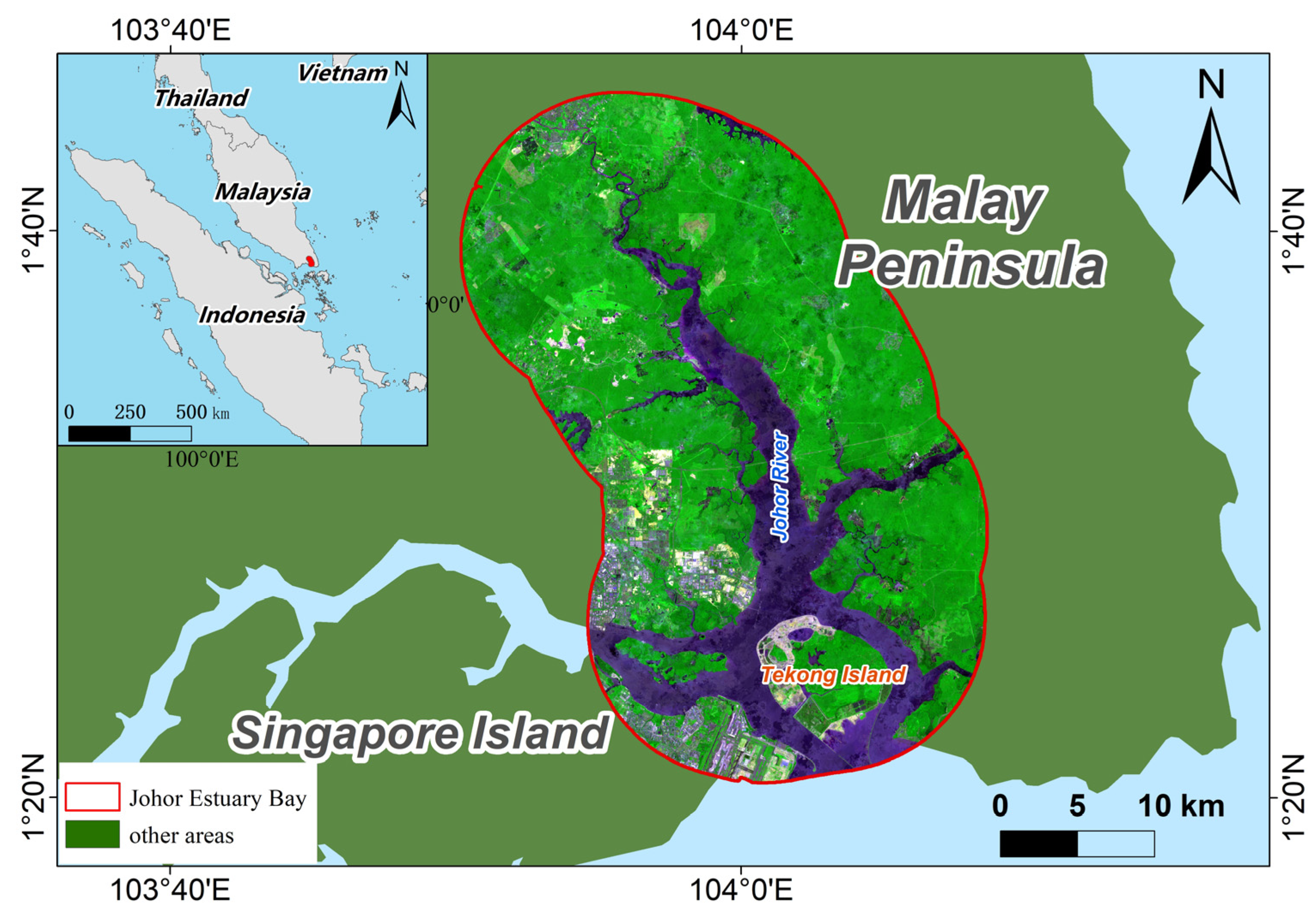
Figure 2.
Distribution of land use in Johor Estuary from 1977 to 2023.
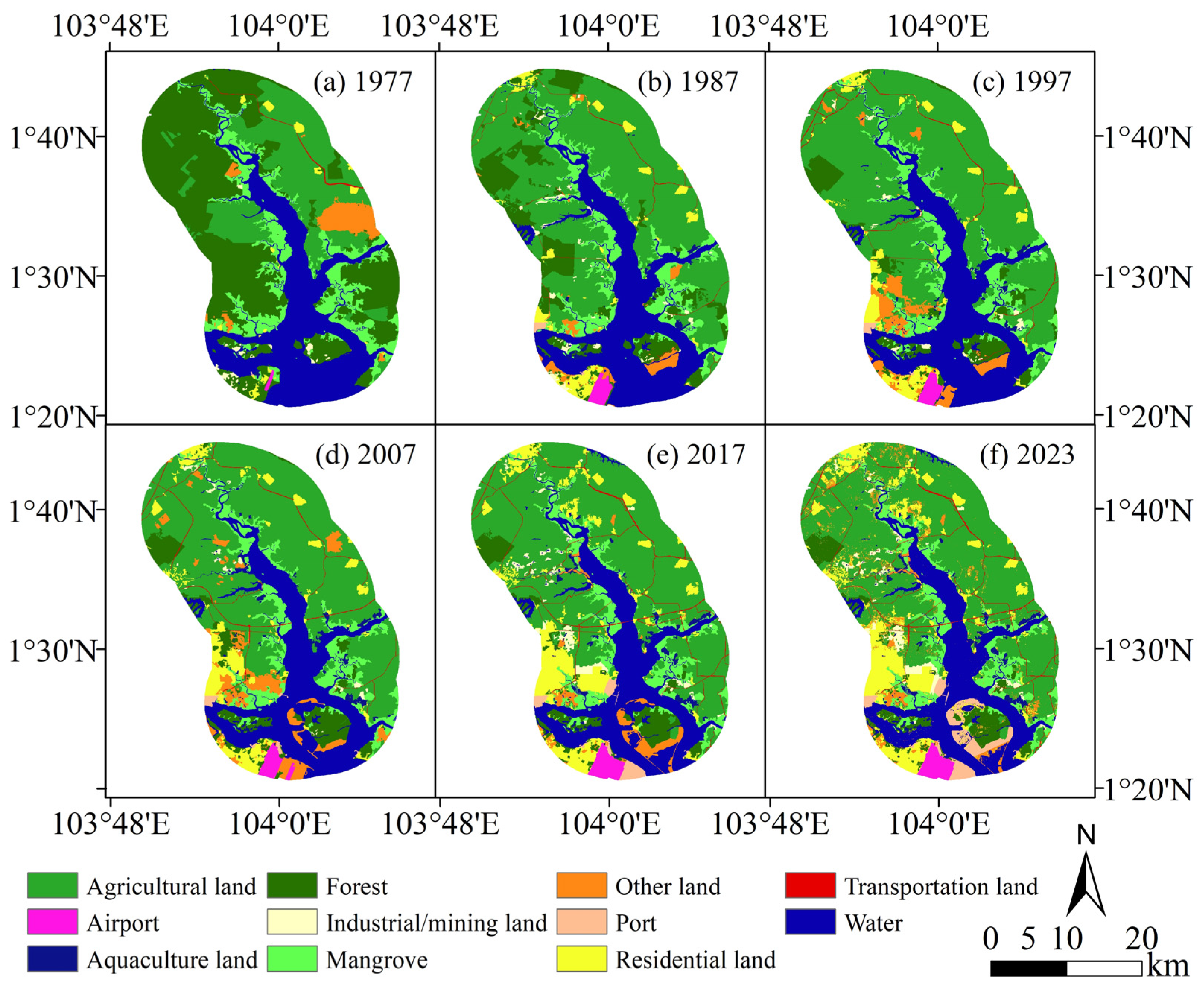
Figure 3.
Land use patterns under different scenarios for 2030.
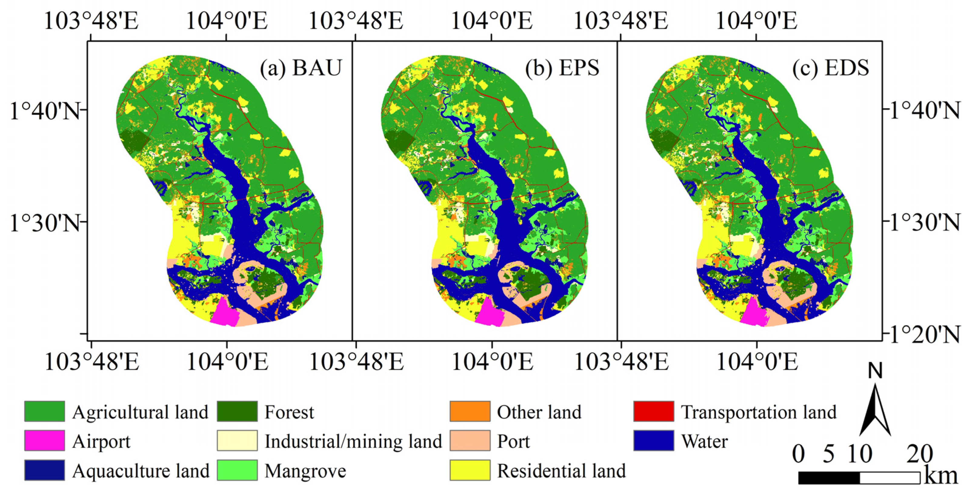
Figure 4.
Area comparison of land types under different scenarios (km2).
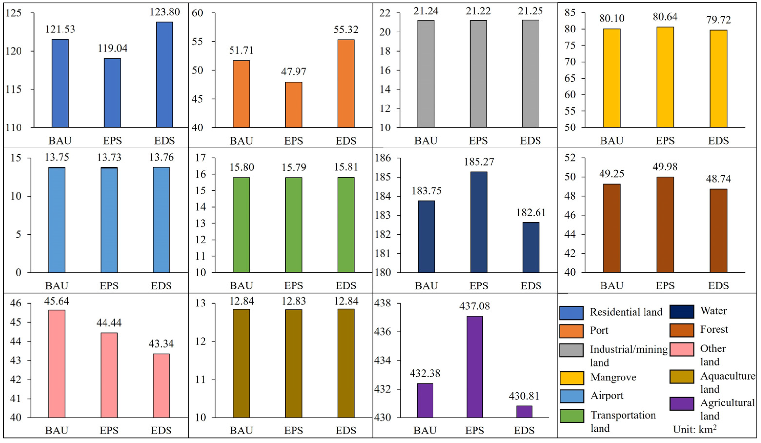
Figure 5.
Distribution pattern of carbon storage in 1977-2023.
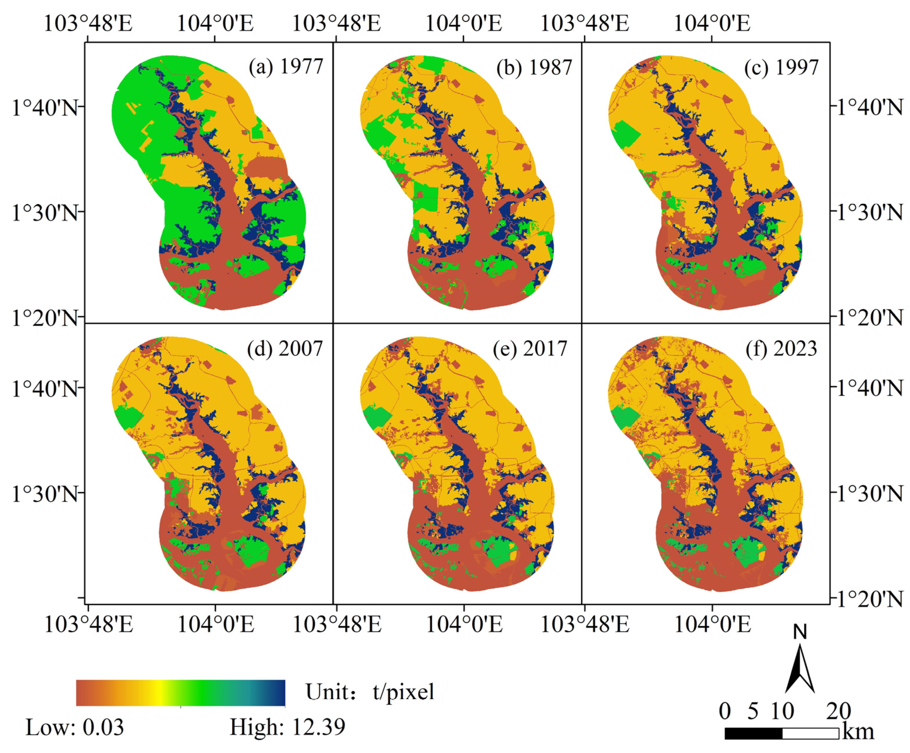
Figure 6.
Patterns of carbon storage variation in 1977-2023.
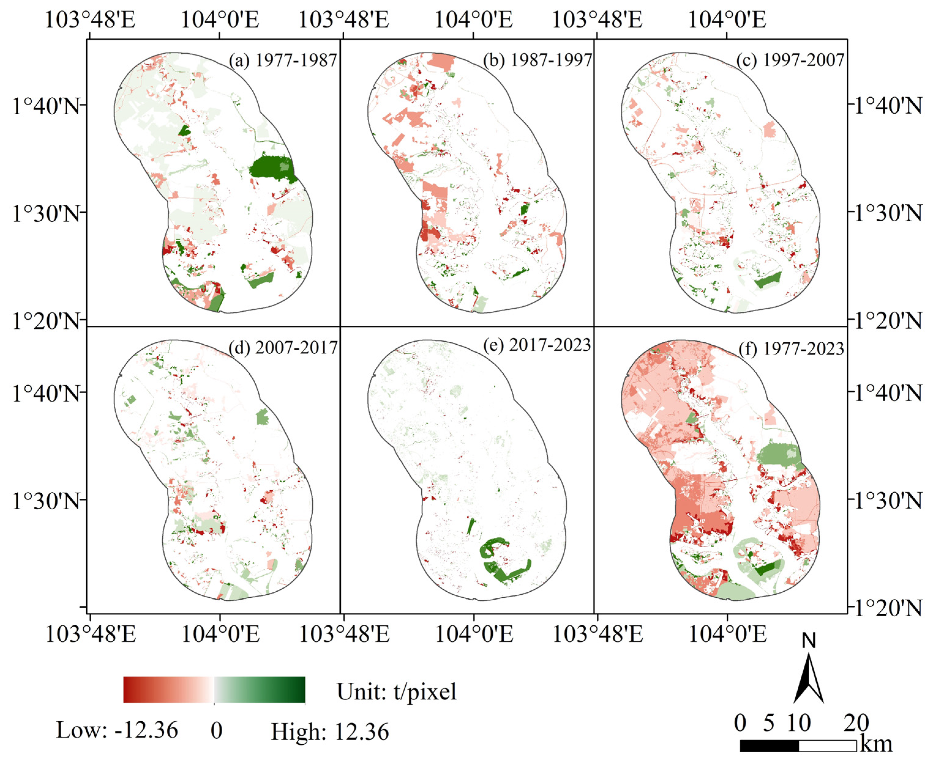
Figure 7.
Distribution pattern of carbon storage in 2030 of three scenarios.
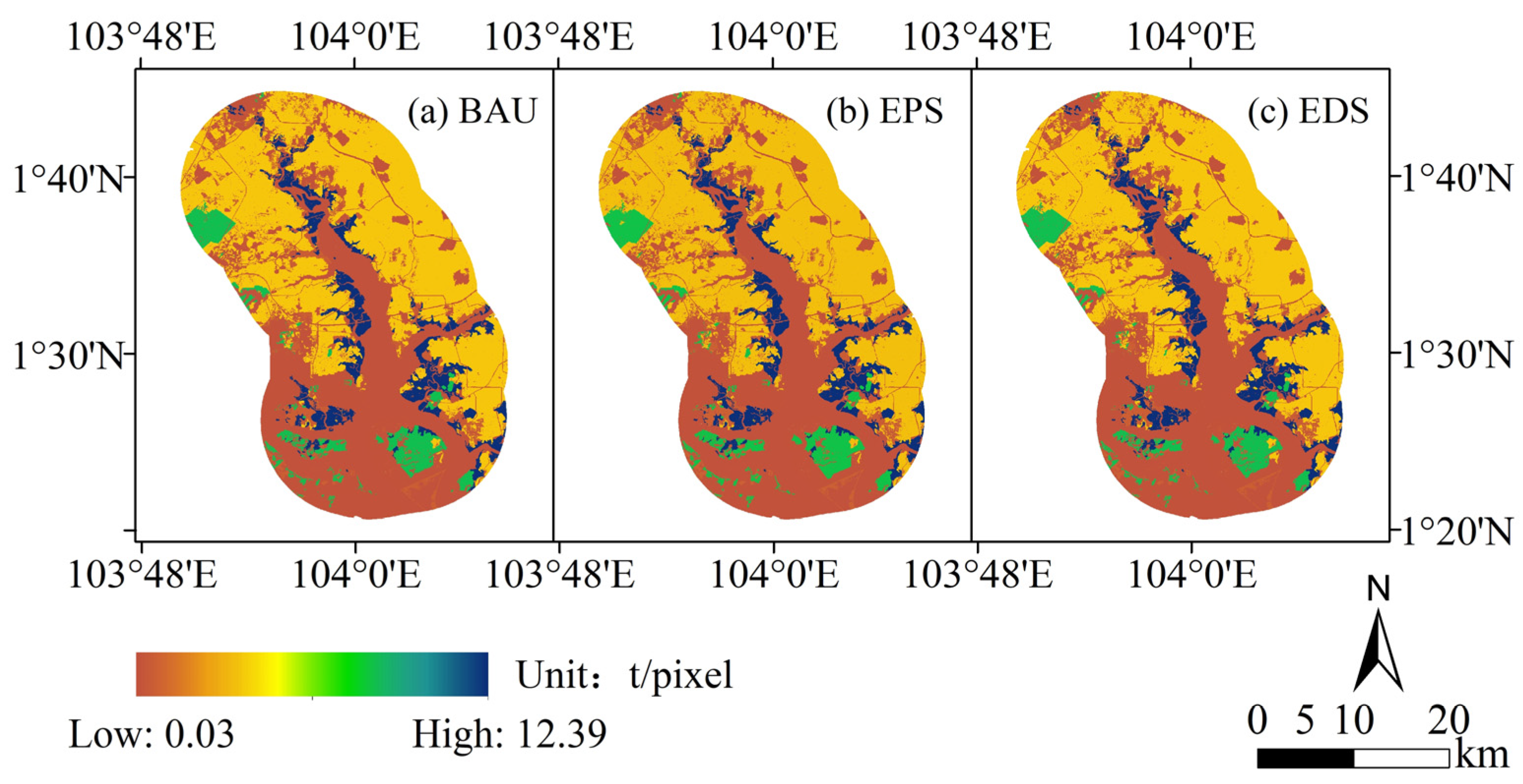
Figure 8.
Total carbon storage in 2023 and 2030 under different scenarios.
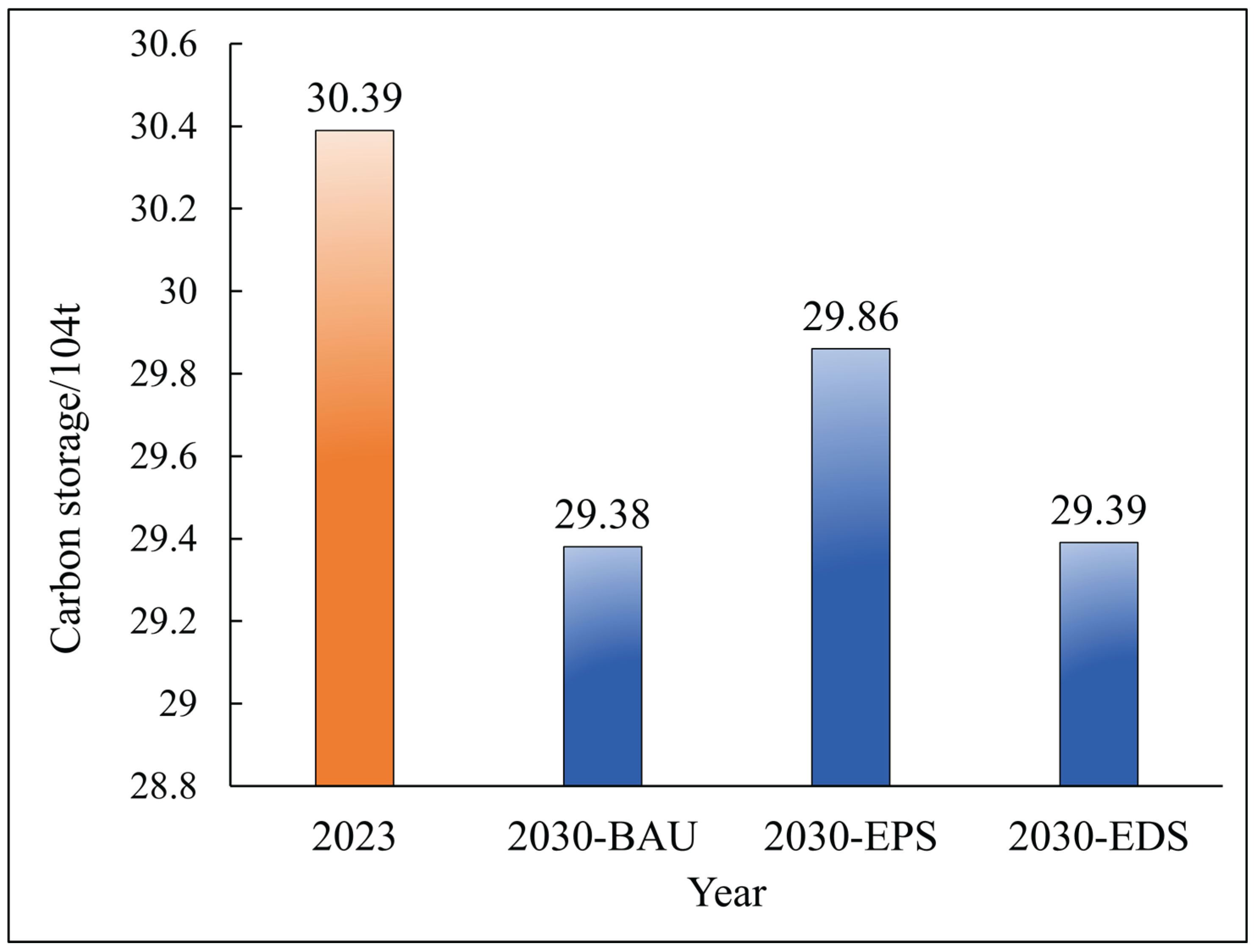
Table 1.
Information of remote sensing images.
| Satellite | Year | Sensor | Image Acquisition Period | Source | |
| Landsat 2-3 | 1977 | MSS | 1975/03/14-1977/06/01 | U.S. Geological Survey (GloVis – USGS) (https://glovis.usgs.gov/) |
|
| Landsat-5 | 1987 | TM | 1987/12/07-1989/09/13 | ||
| 1997 | TM | 1996/12/21-1997/09/03 | / | ||
| 2007 | TM | 2007/05/01-2008/02/22 | |||
| Landsat-8 | 2017 | OLI | 2015/10/23-2017/04/09 | ||
| Sentinel-2 | 2023 | MSI | 2023/01/01-2023/12/31 | Google Earth Engine (GEE) (https://earthengine.google.com/) |
Table 2.
Sources of natural environment and socio-economic data.
| Type | Name | Source |
| Natural Environment Data | DEM | Geospatial Data Cloud (https://www.gscloud.cn/) |
| Bedrock Depth Data | International Soil Reference and Information Centre (ISRIC) Global Soil Data (https://data.isric.org/) | |
| Global Soil Data | Soil and Terrain Database (SOTER) Project (https://data.isric.org/) | |
| Evapotranspiration Data | NASA MODIS Data (https://modis.gsfc.nasa.gov/) | |
| Precipitation Data | Global Precipitation Measurement (GPM) (https://disc.gsfc.nasa.gov/) | |
| Global Annual Mean Temperature Data | National Centers for Environmental Information (NCEI), formerly NCDC (https://www.ncei.noaa.gov/data/) | |
| Socio-economic Data | Road Data | OpenStreetMap (https://www.openstreetmap.org/) |
| Population Density Data | WorldPop (https://www.worldpop.org/) |
Table 3.
Definition and remote sensing features of land-use types.
| Category | Land Type | Definitions | Maps (False color) |
| Construction land | Residential land | Urban and rural land, showing as rough bright white or light gray irregular shapes | 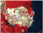 |
| Port | Relatively regular shapes, gray-white color, mainly in coastal and estuarine areas | 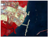 |
|
| Industrial/mining land | Industrial zones and salt pans, gray-white with uneven internal color, relatively clustered | 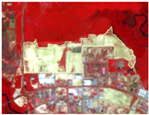 |
|
| Airport | Runways and terminals, regular shapes, gray or smooth light red grassland | 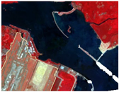 |
|
| Transportation land | Roads outside residential areas, bright white or light gray rough intersecting lines | 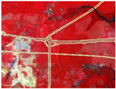 |
|
| Non-construction land | Mangrove | Mostly along coasts, irregular large patches, dark red in images | 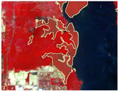 |
| Water | Rivers, lakes, etc., irregular shapes, blue or gray-blue | 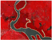 |
|
| Forest | Dark red, rough surface with irregular shapes, large continuous patches | 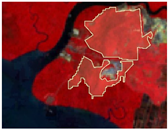 |
|
| Agricultural land | Mostly plantations (rubber and oil palm), red and relatively smooth surface | 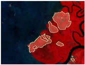 |
|
| Aquaculture land | Mainly aquaculture ponds, deep blue rectangles, including marine and freshwater culture | 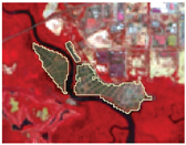 |
|
| Other land | Includes grassland, wasteland, sandy land, mudflats, burned areas, unused land, etc. | 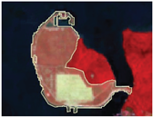 |
Table 4.
Carbon pools of land-use types (t/ha).
| Land Type | Cabove | Cbelow | Csoil | Cdead |
| Residential land | 0.9 | 1.7 | 14 | 0.5 |
| Port | 0.9 | 1.6 | 13.2 | 0.5 |
| Industrial/mining land | 0.9 | 1.6 | 13.2 | 0.5 |
| Mangrove | 142.9 | 18.1 | 1052.9 | 24.95 |
| Airport | 0.9 | 1.6 | 13.2 | 0.5 |
| Transportation land | 0.9 | 1.6 | 13.6 | 0.5 |
| Water | 1.2 | 0.6 | 0.7 | 0.05 |
| Forest | 234.8 | 43.2 | 149.4 | 345 |
| Other land | 7.2 | 18.2 | 37.2 | 2.4 |
| Aquaculture land | 9.2 | 8.6 | 21.3 | 18.5 |
| Agricultural land | 96.73 | 24.91 | 127.1 | 83 |
Table 5.
Percentage of land use types in 1977-2023 (%).
| Land Type | 1977 | 1987 | 1997 | 2007 | 2017 | 2023 |
| Residential land | 0.91 | 3.00 | 4.19 | 5.80 | 9.18 | 10.56 |
| Port | 0.01 | 0.18 | 0.22 | 0.35 | 1.19 | 2.72 |
| Industrial/mining land | 0.49 | 0.99 | 0.57 | 0.54 | 1.70 | 1.87 |
| Mangrove | 12.34 | 9.97 | 9.32 | 9.19 | 8.33 | 8.05 |
| Airport | 0.13 | 0.80 | 0.82 | 0.95 | 1.29 | 1.31 |
| Transportation land | 0.26 | 0.49 | 0.76 | 0.94 | 1.52 | 1.53 |
| Water | 22.89 | 22.20 | 21.70 | 20.30 | 19.38 | 18.61 |
| Forest | 38.93 | 12.55 | 6.15 | 6.78 | 5.48 | 5.13 |
| Other land | 3.16 | 1.90 | 4.12 | 5.18 | 2.36 | 3.89 |
| Aquaculture land | 0.05 | 0.56 | 0.62 | 1.10 | 1.24 | 1.24 |
| Agricultural land | 20.84 | 47.39 | 51.53 | 48.85 | 48.32 | 45.07 |
Table 6.
Variation of CI for land use types from 1977 to 2023 (%).
| Land Type | 1977-1987 | 1987-1997 | 1997-2007 | 2007-2017 | 2017-2023 | 1977-2023 |
| Residential land | 0.11 | 0.28 | 1.65 | 2.27 | 1.28 | 0.41 |
| Port | 0.01 | 0.01 | 0.13 | 0.53 | 1.34 | 0.11 |
| Industrial/mining land | 0.03 | -0.09 | -0.03 | 0.74 | 0.15 | 0.06 |
| Mangrove | -9.09 | -11.03 | -9.63 | -41.87 | -18.77 | -13.33 |
| Airport | 0.03 | <0.01 | 0.13 | 0.22 | 0.02 | 0.05 |
| Transportation land | 0.01 | 0.06 | 0.18 | 0.38 | 0.01 | 0.05 |
| Water | -0.01 | -0.02 | -0.22 | -0.09 | -0.11 | -0.03 |
| Forest | -63.10 | -67.68 | 29.10 | -39.46 | -14.63 | -65.50 |
| Other land | -0.25 | 1.98 | 4.12 | -7.20 | 5.38 | 0.12 |
| Aquaculture land | 0.09 | 0.05 | 1.65 | 0.32 | <0.01 | 0.17 |
| Agricultural land | 27.27 | 18.80 | -53.17 | -6.91 | -58.32 | 20.16 |
Table 7.
Variation of CI for land use types from 1977 to 2023 (%).
| Land Type | BAU | EPS | EDS |
| Residential land | 221.89 | 179.27 | 260.74 |
| Port | 124.19 | -0.95 | 103.93 |
| Industrial/mining land | 27.99 | 28.65 | 32.81 |
| Mangrove | -3282.67 | -67.96 | -3762.66 |
| Airport | 4.62 | 4.25 | -0.82 |
| Transportation land | 1.18 | 1.03 | 1.36 |
| Water | -19.65 | -0.37 | -22.61 |
| Forest | -2689.23 | -351.83 | -3088.86 |
| Other land | 367.06 | 289.44 | 217.91 |
| Aquaculture land | 5.21 | 4.73 | 5.43 |
| Agricultural land | -4833.08 | -5371.98 | -3724.28 |
Disclaimer/Publisher’s Note: The statements, opinions and data contained in all publications are solely those of the individual author(s) and contributor(s) and not of MDPI and/or the editor(s). MDPI and/or the editor(s) disclaim responsibility for any injury to people or property resulting from any ideas, methods, instructions or products referred to in the content. |
© 2025 by the authors. Licensee MDPI, Basel, Switzerland. This article is an open access article distributed under the terms and conditions of the Creative Commons Attribution (CC BY) license (http://creativecommons.org/licenses/by/4.0/).
Copyright: This open access article is published under a Creative Commons CC BY 4.0 license, which permit the free download, distribution, and reuse, provided that the author and preprint are cited in any reuse.


