
Submitted:
12 November 2025
Posted:
12 November 2025
You are already at the latest version
Abstract
This paper presents a cost-effective approach to structural health monitoring (SHM) based on standard image processing and convolutional neural networks (CNNs) for object detection. The proposed algorithm accurately identifies and tracks geometric measurement motives across image sequences, enabling precise position and two-dimensional displacement determination. Experimental investigations using a minimal implementation with open-source Python libraries demonstrate close agreement with reference measurements and low measurement noise. The study also highlights how geometric shape selection, motive arrangement, and preprocessing techniques influence measurement accuracy. This robust, scalable, minimally invasive method offers a low-cost alternative to traditional SHM systems. Its flexibility allows it to be adapted to various infrastructures. Potential future enhancements include strain measurements from multiple motives, multi-plane monitoring, and machine learning–based error correction. These features suggest that the approach is a promising solution for reliable, affordable, and adaptable SHM.
Keywords:
SHM
; displacement measurement
; single camera system
; object detection
; low-cost
1. Introduction
Structural health monitoring (SHM) of infrastructure has become increasingly important and represents an indispensable tool for ensuring the integrity and safety of buildings and civil structures [1,2,3]. In view of recent structural failures such as bridge collapses, continuous monitoring and analysis of structural conditions have gained growing attention in both research and practical applications. Modern infrastructure is exposed to numerous stressors, including excessive use beyond the intended service life, increasing heavy traffic, progressive ageing, and extreme weather events associated with climate change. Consequently, innovative SHM solutions are essential to guarantee the long-term safety and reliability of critical infrastructure. In addition to established SHM methods, new approaches are becoming increasingly relevant. The present study demonstrates the advantages of image-based measurement systems employing standard cameras. These systems are cost-effective, require only simple hardware components, and can operate under varying environmental conditions. They can also be retrofitted into existing monitoring setups, are minimally invasive, and can be implemented using open-source software.
Systematic monitoring of structures, combined with targeted maintenance actions derived from measurement data, contributes significantly to resource conservation and the prevention of potential structural failures [3,4]. Within this context, methods capable of detecting deformations and displacements are of particular scientific and practical relevance. Beyond real-time monitoring, SHM enables data-driven condition forecasting, allowing maintenance intervals and preventive measures to be optimized [5,6]. As modern construction techniques and materials become more widespread, the scalability of monitoring systems—achieved through the integration of distributed measurement points—has become crucial for ensuring adequate surveillance of complex and large-scale structures [7].
A wide range of established techniques exist for monitoring deformations and displacements, each differing in measurement principle, accuracy, and field applicability [8,9,10,11]. Classical methods include strain gauges, which provide direct and highly accurate strain measurements [12]. However, they require direct access to measurement points and are limited to local areas [13]. Fiber optic sensors, particularly spatially resolved systems, have become increasingly popular owing to their ability to measure strain over long distances and their resistance to electromagnetic interference. Fiber Bragg grating sensors allow discrete measurements at defined fiber locations, whereas distributed fiber optic sensors provide continuous strain profiles, enabling both local and global deformation analysis in complex structures [14]. Additional methods include displacement transducers such as inductive, capacitive, and potentiometric sensors [15], which offer high precision at discrete points and are suitable for critical regions. Laser-based sensors provide another contactless alternative, capable of detecting positional changes with high accuracy by measuring the distance to a fixed reflector point [10]. However, they require an unobstructed line of sight. Camera-based techniques have also gained prominence as flexible and versatile tools for displacement detection [10,16,17]. These systems can monitor the movement of entire structural segments, while digital image correlation (DIC) enables high-resolution surface deformation analysis [18]. Such methods capture both local and global displacements, though they rely on adequate image quality and stable environmental conditions. Each monitoring principle offers specific advantages and limitations; therefore, selection of an appropriate method depends on structural characteristics, environmental influences, measurement accuracy, range, and installation effort [3].
Despite the diversity of available techniques, current SHM systems still face technical and practical challenges that restrict their widespread implementation [3,4]. A key limitation lies in the high cost of complex measurement systems [4,19,20], largely due to expensive sensors, specialised hardware components such as interrogators and amplifiers, and maintenance-intensive installations. The integration of sensors and cables—such as fiber optic splicing—requires technical expertise and may introduce installation errors that compromise measurement accuracy. Furthermore, many systems provide single-point measurements, which limits their applicability for large-scale monitoring. Environmental influences such as temperature and humidity variations necessitate compensation procedures, increasing the complexity of data acquisition. Dependence on proprietary software further reduces system flexibility, hinders interoperability between different sensor types, and results in long-term costs due to vendor lock-in [21]. In addition, many sensing systems are mechanically sensitive and unsuitable for continuous operation in harsh environments [22]. Power supply and data transmission present additional challenges for wired systems, as cabling across large structures is logistically demanding and costly [19,21].
To overcome these limitations, cost-effective image-based measurement systems using standard cameras have emerged as a promising alternative [23]. Single-camera setups offer low acquisition costs and eliminate the need for proprietary measuring hardware by employing commercially available industrial or modified digital single-lens reflex (DSLR) cameras [23,24]. Their modular system architecture allows flexible adaptation to various monitoring scenarios, while data processing can rely on open-source algorithms and image analysis methods [25]. A single camera can monitor multiple measurement points simultaneously [26], and specially designed measurement patterns enable sub-micrometre displacement detection [24]. This technique can capture a wide range of structural changes, from simple tilting to complex deformation patterns [11,27]. The use of open-source data analysis tools enhances transparency, adaptability, and independence from proprietary software [28,29]. Furthermore, machine learning algorithms can be incorporated to improve displacement measurement accuracy through automated feature extraction [30]. The combination of low-cost hardware and scalable software allows the establishment of redundant monitoring networks that remain operational under variable environmental conditions. The approach is minimally invasive, as measurement markers can be attached temporarily or permanently to structural surfaces without complex integration. Moreover, it can be retrofitted into existing SHM systems, supporting gradual system expansion.
The present study describes the development and validation of an image-based single-camera system for two-dimensional displacement detection. The objective was to employ a standard industrial camera and a corresponding measurement pattern to record movements along two orthogonal axes with high precision. The system follows a scalable and adaptable design concept suitable for various monitoring applications. An evaluation algorithm was implemented using open-source libraries and tested in a laboratory setup, where a linear translation stage generated controlled displacements of the measurement pattern, serving as a reference system. Laboratory results indicated a high level of agreement between camera-based measurements and reference values. Based on these results, potential improvements, optimization strategies, and remaining challenges for the application of such systems in SHM are discussed.
2. General Considerations
The following section presents the key considerations for determining the position and displacement of measurement motives (MMs) using a basic single-camera system. The proposed method can be readily scaled, optimized, and implemented through open-source algorithms. The approach is structured around four fundamental components:
- Pre-selection of regions of interest (ROIs) based on object detection.
- ROI segmentation.
- Relative and absolute position determination.
- Displacement calculation.
Figure 1 illustrates the basic workflow of the proposed method, and the key considerations for each component are described below.
The measurement sequence depends on the design of the MMs, which fulfills two primary functions. First, it determines the center of gravity, thereby defining the MM’s position within the image. Second, it incorporates known geometric shapes to establish the image scale in the measurement plane. This step is essential for converting pixel-based displacement values into real-world distances.
The target should be designed so that its components can be reliably segmented and identified using standard image-processing techniques. Although no strict design rules exist, simple geometric shapes—such as circles, triangles, or rectangles—are advantageous, as they can be readily distinguished from one another. Double-symmetrical arrangements are generally preferred to enhance robustness.
The required target size depends on the measurement task and imaging parameters, including sensor size, lens characteristics, and measurement distance. The relative size of the target within the image frame strongly influences the accuracy of the evaluation algorithm.
2.1. Pre-Select ROIs Based on Object Detection
The design of suitable MMs provides the foundation for reliable image-based displacement determination. Once an appropriate MM has been defined, the next step involves its detection and localization within recorded images.
Detecting MMs and geometric patterns in large image formats can be challenging, particularly when complex background configurations are present [31]. This difficulty increases when multiple, visually similar MMs must be distinguished. In SHM applications, however, reliable detection and classification of several MMs within large image regions containing busy backgrounds are essential.
To address this challenge, the proposed approach employs object detection based on a convolutional neural network (CNN), which enables simultaneous detection and assignment of multiple motives. A major advantage of this method is that pre-selected ROIs allow processing to be restricted to specific areas, thereby minimizing interference and reducing computational demand.
A CNN is a feedforward neural network that automatically recognizes image features through filter (kernel) optimization and represents a core technique in modern deep learning within the field of machine learning. Several CNN-based object recognition algorithms are available as open-source libraries for common programming languages such as C and Python. The most widely used include Faster R-CNN (Faster Region-Based Convolutional Neural Network), SSD (Single Shot MultiBox Detector), and YOLO (You Only Look Once) [32]. Among these, YOLO currently offers the best performance in terms of speed and reliability, particularly for real-time applications [33]. Nevertheless, the choice of algorithm should be tailored to the specific application context.
The present approach focuses on supporting displacement measurement, where processing efficiency and resource optimization are of particular importance. To date, the MM center cannot be determined with sufficient precision for robust displacement estimation using object detection alone. Therefore, the center of gravity is derived through complementary image-processing methods. Object detection, however, provides essential ROIs and information for plausibility validation.
Furthermore, various MM designs can be linked to a database containing metadata such as the number and dimensions of geometric elements. These values are subsequently used in downstream processing based on the recognized MM identifier. The following parameters are required as outputs of the detection step:
- IDs of detected objects,
- Associated confidence scores,
- Coordinates of bounding boxes, and
- Coordinates of centroids.
2.2. ROI Segmentation
The identified ROIs must be pre-processed before further analysis. Edge detection prior to segmentation improves both accuracy and efficiency. Widely used edge detection algorithms include those developed by Prewitt, Canny, and Sobel [34]. A critical step in edge detection is image smoothing, which reduces noise and softens edge transitions. While smoothing minimizes false edge detection and discontinuities in pixel intensity, it can also result in the loss of important information. Therefore, the choice of smoothing method should be tailored to the application, with median, Gaussian, and bilateral filters being commonly employed. Detailed guidance on algorithm selection, smoothing operations, and input parameters (e.g., kernel size) can be found in the literature [35,36,37,38,39]. The output of this step consists of the preselected ROIs represented as logical matrices.
To assign geometric elements to the MM, closed contours must first be identified within the edge-detected logical matrices. Various contour extraction approaches have been described in the literature [40,41]. Most algorithms trace the outer boundaries of closed regions, allowing the separation of shapes within the ROIs into individual elements. These elements can then be classified based on their geometric properties. Differentiation according to the number of corners is particularly useful, with common detectors including the Harris-Stephens [42,43] and Shi-Tomasi algorithms [44]. For the purposes of this study, determining the number of corners is sufficient, making these approaches adequate. Exact corner localization, as provided by the Förstner algorithm [45], is not required. Elements without corners, such as circles or ellipses, can be categorized based on metrics such as the circumference-to-area ratio or through the Hough transform [46]. Once contours are detected and classified, additional properties, including surface area and geometric centers, can be computed.
A simultaneous plausibility check is performed based on characteristics such as the number of matched geometric shapes, allowing incorrect segmentations to be detected early.
The following parameters are transferred to the next processing step:
- Recognized contours,
- Classification of contours into geometric elements, and
- Geometric properties of the elements (e.g., coordinates of geometric centers, surface area).
2.3. Relative/Absolute Position Determination
The segmentation results are subsequently used to determine the position of each MM relative to its corresponding ROI. Several approaches can be applied for this purpose. The most straightforward method involves calculating the overall center of gravity of all geometric shapes constituting the MM. To enhance accuracy or tailor the position determination to specific applications, the calculation can be restricted to selected shapes only.
Alternative methods include computing the MM center based on the relative distances between individual centroids. The choice of methodology largely depends on the MM design and the symmetry characteristics of its geometric arrangement. Since these approaches rely on averaged values derived from multiple centroids or inter-element distances, position determination can achieve subpixel-level precision.
Finally, the absolute position of each MM center within the overall image is obtained by referencing the ROI coordinates.
2.4. Displacement Calculation
Displacement is determined by comparing the positions of the MMs across multiple input images. The final step involves converting these relative displacements into physical units of length. To achieve this, the relationship between the optical image in the measurement plane and the actual size of the geometric elements on the MM must be established.
This requires precise knowledge of the dimensions of the geometric shapes. One approach is to calculate the ratio of the areas of selected or all elements. Alternatively, distances between the centers or edges of individual elements can be used. Several strategies can yield satisfactory results, allowing optimization for specific measurement tasks.
This calibration step is critical for ensuring measurement accuracy, as even small deviations can cause significant proportional errors. Once calibrated, the MM positions determined at different time points can serve as reference values for a sequence of displacement measurements across multiple images.
3. Experimental Investigations
To evaluate the accuracy and scalability of the proposed measurement algorithm, a minimal experimental setup was implemented. The objective was to design a basic MM and verify the algorithm’s performance using the simplest possible configuration.
3.1. Experimental Design
Measurement motive
As part of the experimental investigations, a simple MM was developed incorporating various geometric shapes. The inclusion of different geometries enabled the assessment of how parameters such as the number of corners and corner angles influence the accuracy of the evaluation algorithm.
The selected configuration consisted of a symmetrical arrangement of right-angled isosceles triangles and rectangles with an aspect ratio of 2:1, combined with a centrally positioned circle (see Figure 2). For testing, the MM was printed on a 4 mm-thick aluminum Dibond panel and mounted onto a linear stage using an aluminum angle bracket. The MM had overall dimensions of 50 mm · 50 mm. Each rectangle measured 10 mm · 5 mm, while the triangles had side lengths of 10 mm. The central circle had a radius of 10 mm.
Test setup
The experimental setup consisted of a rigid frame constructed from aluminum system profiles. The camera was mounted on one side using a bracket made of 15 mm-thick steel plates. On the opposite side, a linear stage was installed to hold the MM via an aluminum angle bracket. The distance between the camera and the MM was 2.35 m.
Two LED spotlights were symmetrically positioned at a distance of 0.87 m from the test object. The illumination was adjusted to achieve an illuminance of 800 lx at a color temperature of 4400 K. The entire frame was vibration-isolated using six steel isolator springs combined with elastomeric bearings. The experiments were conducted in a controlled environment with a constant temperature of 20 ◦C and a relative humidity of 65%. A schematic of the test setup is shown in Figure 3.
A monochrome industrial camera with a 2/3-inch sensor (Basler A2A4200-12gmBAS) was used for image acquisition. The camera was equipped with a fixed focal length lens of 50 mm and an adjustable aperture range of F2.8–F16.0 (Basler C23-5028-5M-P). The sensor (GMAX2509) provides a maximum resolution of 4200 pixels · 2160 pixels, with a 12-bit pixel depth and a pixel size of 2.5 μm · 2.5 μm.
The linear stage featured a bidirectional repeatability of 0.8 μm and was equipped with a linear encoder offering a resolution of 80. Owing to its high precision, the encoder readings were used as the position reference for all measurements. A stepped motion profile was applied, consisting of five displacement steps of 1.5 mm in both the positive and negative directions. Each position was held for 170 s, resulting in a total test duration of 60 min. The corresponding displacement path recorded by the stage’s linear encoder is shown in Figure 4. A separate data recorder was used to synchronously capture both the camera images and the encoder readings at intervals of 5 s.
3.2. Minimal Implementation of the Algorithm
To verify the functionality of the proposed approach, a minimal implementation of the measurement algorithm described in Section 2 was developed. The algorithm was fully implemented in Python and leverages the following libraries:
- ultralytics (8.3.99)
- torch (2.6.0+cu126)
- opencv-python (4.10.0.84)
- numpy (1.26.4)
The subsequent paragraphs describe the individual components and functions of the algorithm, illustrating how object detection, ROI segmentation, geometric analysis, and displacement computation are implemented in this minimal example.
CNN object detection
For object detection, the real-time YOLO series detector (Generation 11) was employed. This CNN from Ultralytics is licensed under AGPL 3.0, permitting free non-commercial use. A custom dataset of 253 images was created to train the model, containing various scenes both with and without the MM present. The dataset was split into 222 training images and 31 validation images.
The model for this minimal implementation was trained using the pretrained YOLO11l network, which is based on the COCO dataset. Training was performed over 200 epochs with a target image size of 1024 pixels.
ROI Segmentation
Only the ROIs identified by the object detection step were used for further processing. This significantly reduces computational load by limiting the analysis to a small section of the image. Given the MM’s illumination and the high resolution of the camera sensor, a median filter (cv2.medianBlur()) with a pixel window was applied to reduce noise. Edge detection was then performed on the filtered ROI using the Canny algorithm (cv2.Canny()) with gradient thresholds of 100 and 200.
Contour detection was performed using OpenCV’s findContours() function, based on [47]. The retrieval mode was set to RETR_EXTERNAL to consider only outer contour points, and the approximation method was set to CHAIN_APPROX_NONE to preserve all contour points. This function returns nested arrays of closed contours, which were iterated to classify individual shapes:
- General
- Contours with an area smaller than 100 pixels were ignored to reduce noise-related false detections. This threshold should be adjusted according to the expected minimum size of the geometric shapes.
- Circles
- Circularity was calculated aswhere A is the area and P is the perimeter of the contour [48]. A perfect circle has a circularity of 1. Shapes with circularity above 0.85 were classified as circles, based on empirical tuning for the test setup.
- Polygons
- Triangles and rectangles were identified using the Ramer-Douglas-Peucker algorithm, implemented via approxPolyDP() [49,50], which approximates a curve by reducing the number of points. The approximation tolerance was set to 10% of the contour perimeter. The number of corners in each polygon was determined from the resulting array of approximated points. This method is robust for the current setup, though alternative corner detection algorithms may be preferred for different applications.
Finally, centroids were computed for all classified contours using image moments, and a plausibility check was performed by verifying the expected number of shapes in each category (one circle, four triangles, and four rectangles).
Relative/Absolute Position Determination
Two approaches were used to determine the overall center of gravity of the MM. First, the arithmetic mean of all shape centroids was calculated. Second, the center of gravity was calculated separately for each type of geometric shape. The nomenclature for these approaches is summarized in Table 1.
The relative coordinates of the center of gravity within the ROI can then be converted to absolute positions in the overall image by incorporating the ROI coordinates.
Image Scale Determination
Three approaches were used to determine the image scale:
- Area
- The simplest method is to compare the actual size of the geometric shapes on the MM with the size of the enclosed area of the classified contours:where is the contour area in pixels and A is the actual area of the corresponding shape.
- Circles
- Circular shapes can be used by comparing parameters such as radius, circumference, or area. Here, the radius was determined using the OpenCV function minEnclosingCircle() on contours classified as circles. The actual circle radius is 10 mm.
- Polygons
- In this approach, the image scale is determined by comparing the distances between centroids of the triangles and rectangles. The distances between the triangle centroids are 26.667 mm for adjacent elements and 37.712 mm for opposite elements. For rectangles, the distances are 24.749 mm for adjacent elements and 35 mm for opposite elements. The overall scale factor is calculated using the mean of all respective shape ratios.
Table 2 summarizes the nomenclature for the individual image scale determination approaches.
Displacement Measurement
Finally, the displacements were determined by comparing the MM positions across multiple images and converting them into physical units using the corresponding image scale factor. Different combinations of position determination and image scale calculation were considered, as summarized in Table 3.
4. Results
4.1. Object Detection
Object detection yielded satisfactory results across the entire dataset, achieving an average confidence score of 0.899. The detection quality, however, varied slightly depending on the position of the measurement target, as illustrated in Figure 5.
4.2. Filtering and Edge Detection
Figure 6 shows the ROI of the detected MM, on which edge detection was applied to the initial measurement image.
The application of a median filter results in smooth contours and effectively reduces noise. However, some sharp corners are slightly rounded, and minor rounding of edges can be observed.
4.3. Segmentation
The segmentation results were consistently reliable across the entire dataset. For each image, the correct number of closed contours was detected and successfully classified into geometric shapes. The plausibility checks confirmed that the expected number of circles, triangles, and rectangles were identified in all cases. This indicates that the chosen threshold value for corner detection is appropriate for the applied setup.
Figure 7 illustrates an example of the segmented geometric elements within the MM in the overall image.
4.4. Determination of Motive Position
The centroids of the geometric shapes in the MM were determined using image moments. Figure 8 shows the categorized shapes and their centroids for the first image.
Figure 9 compares the absolute centroid positions for each shape category over the measurement period before the first displacement step. Noise remains in the subpixel range. Circle and rectangle centroids are closely aligned, while triangle centroids exhibit larger deviations, influencing the overall arithmetic mean of all elements.
4.5. Determination of the Image Scale
The image scale was calculated from the geometric elements in the MM to convert pixel displacements into physical units. Figure 10 shows the resulting image scale values for the different approaches across the dataset. Mean values and standard deviations are summarized in Table 4.
Several observations can be made: the methods based on the area of all shapes (pxsza) and the circle diameter (pxszc) exhibit slightly lower values and higher variability compared to the centroid-distance approaches. In contrast, the scales determined from the distances between rectangle (pxszr) and triangle (pxszt) centroids are closely aligned and show minimal scatter. Overall, the centroid-distance methods provide the most consistent and reliable image scale for subsequent displacement measurements.
4.6. Displacement Measurement
Table 3 summarizes the combinations of position determination and image scale calculation methods used for displacement measurements. For consistency, combinations were chosen so that the same geometric shapes are used for position and scale determination.
First, displacements were calculated solely using circles (dispc), then using triangles (dispt) or rectangles (dispr). Finally, mixed combinations of position and scale from triangles and rectangles were used (disptr and disprt). Figure 11 compares the X-direction displacements for the first five steps.
Displacements calculated solely from rectangles (dispr) show the best agreement with reference values, with deviations typically below ±10 μm even at large displacement steps. Measurement uncertainty remains low across all ranges, with an extended uncertainty below 0.6 μm (Figure 12 and Figure 13).
Displacements determined using triangles (dispt) exhibit moderate absolute deviations that vary with the displacement magnitude. While individual steps show low scatter, the overall accuracy is limited by a scaling-factor effect (Figure 14 and Figure 15). Uncertainty increases with displacement.
Mixed methods (disptr and disprt) produce intermediate deviations. Absolute deviations are moderate, but disptr shows asymmetrical deviations: negative X shifts produce larger errors than positive shifts (Figure 16 and Figure 17). In contrast, disprt exhibits a more balanced distribution of deviations (Figure 18 and Figure 19).
Measurements based solely on circles (dispc) and on the areas of all elements (dispa) showed large deviations from the reference values and high variability across all displacement steps; consequently, they were not investigated further, as they do not provide reliable displacement information. Figure 20 provides an overview of the absolute deviations for all examined methods based on polygons. Overall, rectangle-based methods provide the highest accuracy and lowest measurement uncertainty, triangle-based methods reveal scaling-dependent deviations, and circle-based measurements are least reliable.
5. Discussion
The experimental investigations demonstrate that the developed image-based approach enables accurate and stable displacement measurements, even when implemented with a minimal setup. The CNN-based object detection provided high confidence values and reliable identification of MMs, despite a limited training dataset. The minor fluctuations observed in confidence levels likely result from positional dependencies and limited training diversity, but they do not significantly influence subsequent processing or measurement quality.
Edge detection within the extracted ROIs yielded robust contour recognition for all geometric elements. Nevertheless, information loss occurred at edges and corners due to preprocessing with a median filter and the Gaussian filter embedded in the cv.Canny() function. These filters effectively reduced noise and improved contour smoothness but caused rounded corners and slight edge shifts. As a result, the detected edges deviate marginally from their actual course, introducing minor inaccuracies in size and centroid estimation. However, since this effect is consistent across all edges, its influence on centroid determination is minimal—particularly for double-symmetrical shapes such as rectangles. For asymmetrical geometries, such as triangles, this loss of information has a stronger effect on the calculated centroid and, consequently, on the derived distances and scale factors.
As shown in the results, the determination of the MM’s absolute position within the image is highly stable, exhibiting deviations of approximately 0.3 pixels (34 μm) in the X direction and 0.2 pixels (23 μm) in the Y direction between the applied position determination methods. This confirms that, in bilaterally symmetrical configurations, geometric variations have only a negligible influence on positional accuracy. Notably, these deviations correspond to absolute offsets rather than multiplicative (factorial) errors and therefore remain nearly constant across successive displacement steps. Consequently, their impact on displacement determination is minimal, as the relative positional relationships are preserved throughout the measurement sequence.
In contrast, deviations in image scale determination have a considerably stronger effect, since they introduce multiplicative errors that scale proportionally with the measured displacements. Variations in scale calibration of up to 4.5 μm per pixel were observed, substantially influencing the computed displacement values and representing the dominant source of measurement uncertainty. The influence of these distinct error types becomes particularly apparent in the displacement evaluation, where the stability of positional determination and the accuracy of scale calibration jointly define the achievable measurement precision. This effect becomes evident in the displacement results. Rectangle-based methods (dispr) show the best correlation with the reference system, achieving deviations within ±10 μm and extended uncertainties below 1 μm. Given a maximum reference displacement of 7.5 mm, this corresponds to a relative deviation of less than ±0.15%, which is highly promising for such a minimal implementation. The high accuracy is primarily attributed to the geometric stability of double-symmetrical shapes and the reduced centroid sensitivity to filtering effects. In contrast, triangle- and circle-based measurements exhibit scale-dependent deviations arising from slight inconsistencies in image scale determination.
The observed symmetry of the deviation curves indicates that most systematic errors are linked to the scaling factor rather than to random noise. The sign reversal of deviations between positive and negative displacements reflects a slight underestimation or overestimation of the scale factor depending on displacement direction. Asymmetrical effects—such as in disptr—are likely caused by lighting variations, partial shading on the printed MMs, or minimal angular misalignments in the setup.
It must be emphasized that all results were obtained under controlled laboratory conditions. Under real-world conditions, numerous environmental and optical influences—such as variable lighting, direct sunlight reflections, shadows, air shimmer due to local temperature gradients, fog, increased humidity, and airborne particles—can significantly affect optical measurements. These influences are not specific to this system but affect all optical SHM approaches [4,10]. Future research should focus on detecting and compensating for these effects, possibly through adaptive preprocessing, calibration routines, or machine learning–based correction algorithms.
Beyond field applications, the approach also offers high potential for laboratory use. Due to its precision, modularity, and open-source implementation, it is particularly suited for experimental investigations and validation tasks. The simplicity of the setup combined with the low cost of standard cameras and Python-based processing makes it ideal for cost-sensitive research environments where high spatial accuracy and scalability are required.
The accuracy of the displacement results is also influenced by the distance between the camera and the measurement motives. A larger distance generally leads to a reduction in precision due to the lower resolution of the captured image and the effects of angular distortion [11,25]. Furthermore, the size of the measurement motives also plays a crucial role in the overall measurement accuracy. Larger measurement motives typically provide higher precision since they offer more visual information to detect and track, thus reducing relative errors in position determination [18,28].
The camera fixture and its stability during measurements are another critical factor. Small shifts or rotations of the camera during the measurement process can lead to substantial measurement errors due to the geometric distortions that arise from even slight changes in angle or distance [17]. Additionally, vibrations and other mechanical disturbances can induce temporary errors, which would compromise measurement accuracy. Therefore, ensuring the stability of the camera setup is essential for continuous, reliable measurements. This highlights the need for secure mounting and vibration dampening when conducting measurements in real-world conditions, where environmental factors such as building movements or traffic can induce micro-movements in the measurement system [4]. Thus, it would be important to consider the setup’s stability when planning a measurement campaign.
In addition to mechanical stability, the geometric alignment between the camera and the measurement plane is a crucial factor for ensuring measurement accuracy. In the present minimal implementation, the measurement plane must be positioned approximately perpendicular to the camera’s optical axis to avoid perspective-induced distortions. Any deviation from this orthogonal alignment leads to non-uniform image scaling and apparent shape deformation, which can affect both position and scale estimations. To compensate for such misalignments, corrective procedures can be applied, for instance, by comparing the apparent sizes of multiple MMs of identical geometry across the field of view. From these relative differences, an alignment correction factor can be derived. More advanced strategies may include reciprocal weighting of the individual elements or geometric calibration based on known reference distances, which would enable accurate displacement estimation even under non-ideal viewing conditions.
The experimental results further confirm that the accuracy of the proposed measurement approach is primarily determined by the robustness of image scale estimation, the symmetry of the measurement motive, and the consistency of preprocessing filters. However, for long-term SHM applications, it is essential to address potential sources of error and investigate solutions for compensating for environmental influences, camera fixture instability, and other real-world challenges. These findings form the basis for further improvements and extensions, such as the integration of strain measurements and multi-plane displacement measurements, which could significantly enhance the approach’s applicability and versatility.
6. Conclusions
This study presented the development and validation of a simple yet precise image-based algorithm for two-dimensional displacement measurement using standard cameras and open-source software. The algorithm combines CNN-based object detection with classical image processing methods for contour and centroid determination, enabling automated, cost-efficient, and scalable displacement monitoring.
Even in its minimal implementation, the system achieved high accuracy. The configuration using double-symmetrical rectangular motives (dispr) produced the most accurate and stable results, with maximum deviations below ±10 μm at a reference displacement of 7.5 mm, corresponding to a relative deviation below ±0.15%. This demonstrates the method’s high potential for precise and repeatable displacement detection without specialized hardware or proprietary software.
The investigations further showed that the geometric design of the measurement motives significantly affects accuracy. Double-symmetrical geometries such as rectangles proved particularly robust against edge-related information losses during filtering, whereas triangular and mixed configurations exhibited systematic scaling effects. The use of open-source Python-based libraries enables full transparency, adaptability, and scalability of the algorithm for diverse monitoring applications.
Overall, the findings highlight that low-cost, image-based measurement systems can provide accuracy and reliability comparable to more complex sensor systems. Such methods represent a cost-effective, minimally invasive, and scalable alternative for SHM [4,10,21], while also offering value for laboratory applications requiring flexible experimental setups and reproducible results.
Future work should address field implementation by developing robust compensation methods for environmental and optical effects, such as variable illumination, air turbulence, or humidity changes. Furthermore, extending the algorithm to enable strain analysis from multiple measurement motives and incorporating displacement evaluation across different planes will further enhance its practical applicability and relevance for both SHM and experimental research.
References
- Nithin, T.A. Real-time structural health monitoring: An innovative approach to ensuring the durability and safety of structures. 11, 43. [CrossRef]
- Brownjohn, J. Structural health monitoring of civil infrastructure. 365, 589–622. [CrossRef] [PubMed]
- Aktan, E.; Bartoli, I.; Glišić, B.; Rainieri, C. Lessons from Bridge Structural Health Monitoring (SHM) and Their Implications for the Development of Cyber-Physical Systems. 9, 30. [CrossRef]
- Farrar, C.R.; Worden, K. An introduction to structural health monitoring. 365, 303–315. [CrossRef]
- Rabi, R.R.; Vailati, M.; Monti, G. Effectiveness of Vibration-Based Techniques for Damage Localization and Lifetime Prediction in Structural Health Monitoring of Bridges: A Comprehensive Review. 14, 1183. [CrossRef]
- Anjum, A.; Hrairi, M.; Aabid, A.; Yatim, N.; Ali, M. Civil Structural Health Monitoring and Machine Learning: A Comprehensive Review. 18, 43–59. [CrossRef]
- Laflamme, S.; Ubertini, F.; Di Matteo, A.; Pirrotta, A.; Perry, M.; Fu, Y.; Li, J.; Wang, H.; Hoang, T.; Glisic, B.; et al. Roadmap on measurement technologies for next generation structural health monitoring systems. 34, 093001. [CrossRef]
- Gharehbaghi, V.R.; Noroozinejad Farsangi, E.; Noori, M.; Yang, T.Y.; Li, S.; Nguyen, A.; Málaga-Chuquitaype, C.; Gardoni, P.; Mirjalili, S. A Critical Review on Structural Health Monitoring: Definitions, Methods, and Perspectives. 29, 2209–2235. [CrossRef]
- Hassani, S.; Dackermann, U. A Systematic Review of Optimization Algorithms for Structural Health Monitoring and Optimal Sensor Placement. 23, 3293. [CrossRef]
- Kot, P.; Muradov, M.; Gkantou, M.; Kamaris, G.S.; Hashim, K.; Yeboah, D. Recent Advancements in Non-Destructive Testing Techniques for Structural Health Monitoring. 11, 2750. [CrossRef]
- Palma, P.; Steiger, R. Structural health monitoring of timber structures – Review of available methods and case studies. 248, 118528. [CrossRef]
- dos Reis, J.; Oliveira Costa, C.; Sá da Costa, J. Strain gauges debonding fault detection for structural health monitoring. 25, e2264. [CrossRef]
- Bolandi, H.; Lajnef, N.; Jiao, P.; Barri, K.; Hasni, H.; Alavi, A.H. A Novel Data Reduction Approach for Structural Health Monitoring Systems. 19, 4823. [CrossRef] [PubMed]
- Weisbrich, M.; Holschemacher, K.; Bier, T. Comparison of different fiber coatings for distributed strain measurement in cementitious matrices. 9, 189–197. [CrossRef]
- Scuro, C.; Lamonaca, F.; Porzio, S.; Milani, G.; Olivito, R. Internet of Things (IoT) for masonry structural health monitoring (SHM): Overview and examples of innovative systems. 290, 123092. [CrossRef]
- Kim, J.W.; Choi, H.W.; Kim, S.K.; Na, W.S. Review of Image-Processing-Based Technology for Structural Health Monitoring of Civil Infrastructures. 10, 93. [CrossRef]
- Dong, C.Z.; Catbas, F.N. A review of computer vision–based structural health monitoring at local and global levels. 20, 692–743. [CrossRef]
- Boursier Niutta, C.; Tridello, A.; Ciardiello, R.; Paolino, D.S. Strain Measurement with Optic Fibers for Structural Health Monitoring of Woven Composites: Comparison with Strain Gauges and Digital Image Correlation Measurements. 23, 9794. [CrossRef]
- Morgenthal, G.; Eick, J.F.; Rau, S.; Taraben, J. Wireless Sensor Networks Composed of Standard Microcomputers and Smartphones for Applications in Structural Health Monitoring. 19, 2070. [CrossRef]
- Mustapha, S.; Lu, Y.; Ng, C.T.; Malinowski, P. Sensor Networks for Structures Health Monitoring: Placement, Implementations, and Challenges—A Review. 4, 551–585. [CrossRef]
- Malik, H.; Khattak, K.S.; Wiqar, T.; Khan, Z.H.; Altamimi, A.B. Low Cost Internet of Things Platform for Structural Health Monitoring. In Proceedings of the 2019 22nd International Multitopic Conference (INMIC); IEEE. [CrossRef]
- Kralovec, C.; Schagerl, M. Review of Structural Health Monitoring Methods Regarding a Multi-Sensor Approach for Damage Assessment of Metal and Composite Structures. 20, 826. [CrossRef]
- Sony, S.; Laventure, S.; Sadhu, A. A literature review of next-generation smart sensing technology in structural health monitoring. 26, e2321. [CrossRef]
- Feng, D.; Feng, M.; Ozer, E.; Fukuda, Y. A Vision-Based Sensor for Noncontact Structural Displacement Measurement. 15, 16557–16575. [CrossRef]
- Henke, K.; Pawlowski, R.; Schregle, P.; Winter, S. Use of digital image processing in the monitoring of deformations in building structures. 5, 141–152. [CrossRef]
- Ye, X.W.; Dong, C.Z.; Liu, T. A Review of Machine Vision-Based Structural Health Monitoring: Methodologies and Applications 2016, 1–10. [CrossRef]
- Feng, D.; Feng, M.Q. Experimental validation of cost-effective vision-based structural health monitoring. 88, 199–211. [CrossRef]
- Chen, B.; Tomizuka, M. OpenSHM: Open Architecture Design of Structural Health Monitoring Software in Wireless Sensor Nodes. In Proceedings of the 2008 IEEE/ASME International Conference on Mechtronic and Embedded Systems and Applications. IEEE; pp. 19–24. [CrossRef]
- Basto, C.; Pelà, L.; Chacón, R. Open-source digital technologies for low-cost monitoring of historical constructions. 25, 31–40. [CrossRef]
- Xu, Q.; Wang, X.; Yan, F.; Zeng, Z. Non-Contact Extensometer Deformation Detection via Deep Learning and Edge Feature Analysis. In Design Studies and Intelligence Engineering; IOS Press. [CrossRef]
- Peters, J.F. Foundations of Computer Vision. [CrossRef] [PubMed]
- Aboyomi, D.D.; Daniel, C. A Comparative Analysis of Modern Object Detection Algorithms: YOLO vs. SSD vs. Faster R-CNN. 8, 96–106. [CrossRef]
- Bilous, N.; Malko, V.; Frohme, M.; Nechyporenko, A. Comparison of CNN-Based Architectures for Detection of Different Object Classes. 5, 2300–2320. [CrossRef]
- Kumari, R.; Chandra, D. Real-time Comparison of Performance Analysis of Various Edge Detection Techniques Based on Imagery Data. 42, 22–31. [CrossRef]
- Li, P.; Wang, H.; Yu, M.; Li, Y. Overview of Image Smoothing Algorithms. 1883, 012024. [Google Scholar] [CrossRef]
- Chen, B.H.; Tseng, Y.S.; Yin, J.L. Gaussian-Adaptive Bilateral Filter. 27, 1670–1674. [CrossRef]
- Shreyamsha Kumar, B.K. Image denoising based on gaussian/bilateral filter and its method noise thresholding. 7, 1159–1172. [CrossRef]
- Das, S. Comparison of Various Edge Detection Technique. 9, 143–158. [CrossRef]
- Magnier, B.; Abdulrahman, H.; Montesinos, P. A Review of Supervised Edge Detection Evaluation Methods and an Objective Comparison of Filtering Gradient Computations Using Hysteresis Thresholds. 4, 74. [CrossRef]
- Yang, D.; Peng, B.; Al-Huda, Z.; Malik, A.; Zhai, D. An overview of edge and object contour detection. 488, 470–493. [CrossRef]
- Papari, G.; Petkov, N. Edge and line oriented contour detection: State of the art. 29, 79–103. [CrossRef]
- Harris, C.; Stephens, M. A Combined Corner and Edge Detector; pp. 23.1–23.6. [CrossRef]
- Sánchez, J.; Monzón, N.; Salgado, A. An Analysis and Implementation of the Harris Corner Detector. 8, 305–328. [CrossRef]
- Shi, J.; Tomasi. Good features to track; pp. 593–600. [CrossRef]
- Förstner, W.; Gülch, E. A Fast Operator for Detection and Precise Location of Distict Point, Corners and Centres of Circular Features.
- Illingworth, J.; Kittler, J. The Adaptive Hough Transform. PAMI- 9 690–698. [CrossRef] [PubMed]
- Suzuki, S.; be, K. Topological structural analysis of digitized binary images by border following. 30, 32–46. [CrossRef]
- Montero, R.S.; Bribiesca, E. State of the Art of Compactness and Circularity Measures; 2009. [Google Scholar]
- Ramer, U. An iterative procedure for the polygonal approximation of plane curves. 1, 244–256. [CrossRef]
- Douglas, D.H.; Peucker, T.K. Algorithms for the Reduction of the Number of Points Required to Represent a Digitized Line or its Caricature; pp. 15–28. [CrossRef]
Figure 1.
Basic workflow.
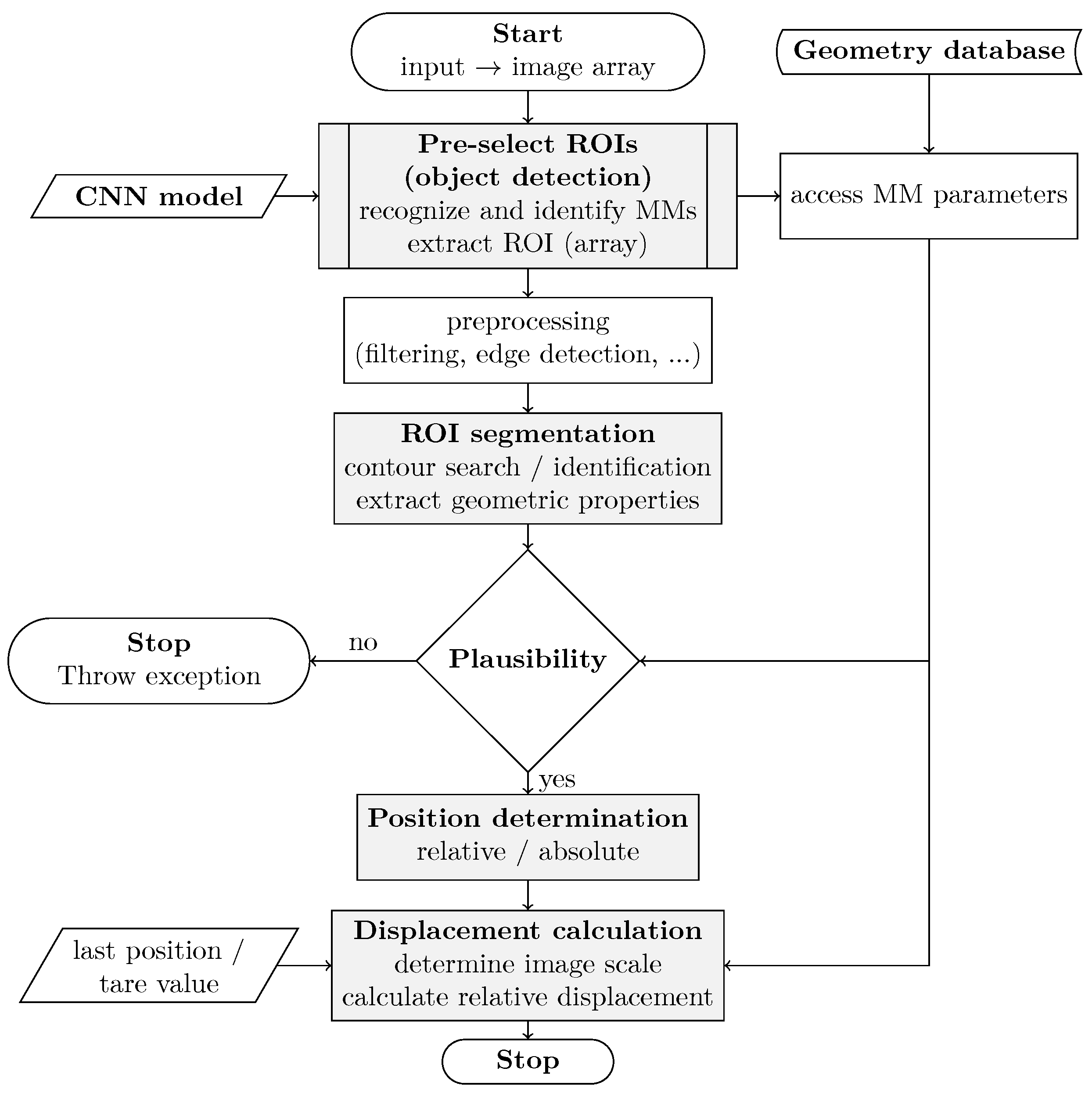
Figure 2.
(a) Measurement motive (MM); (b) dimensioned representation of the MM.
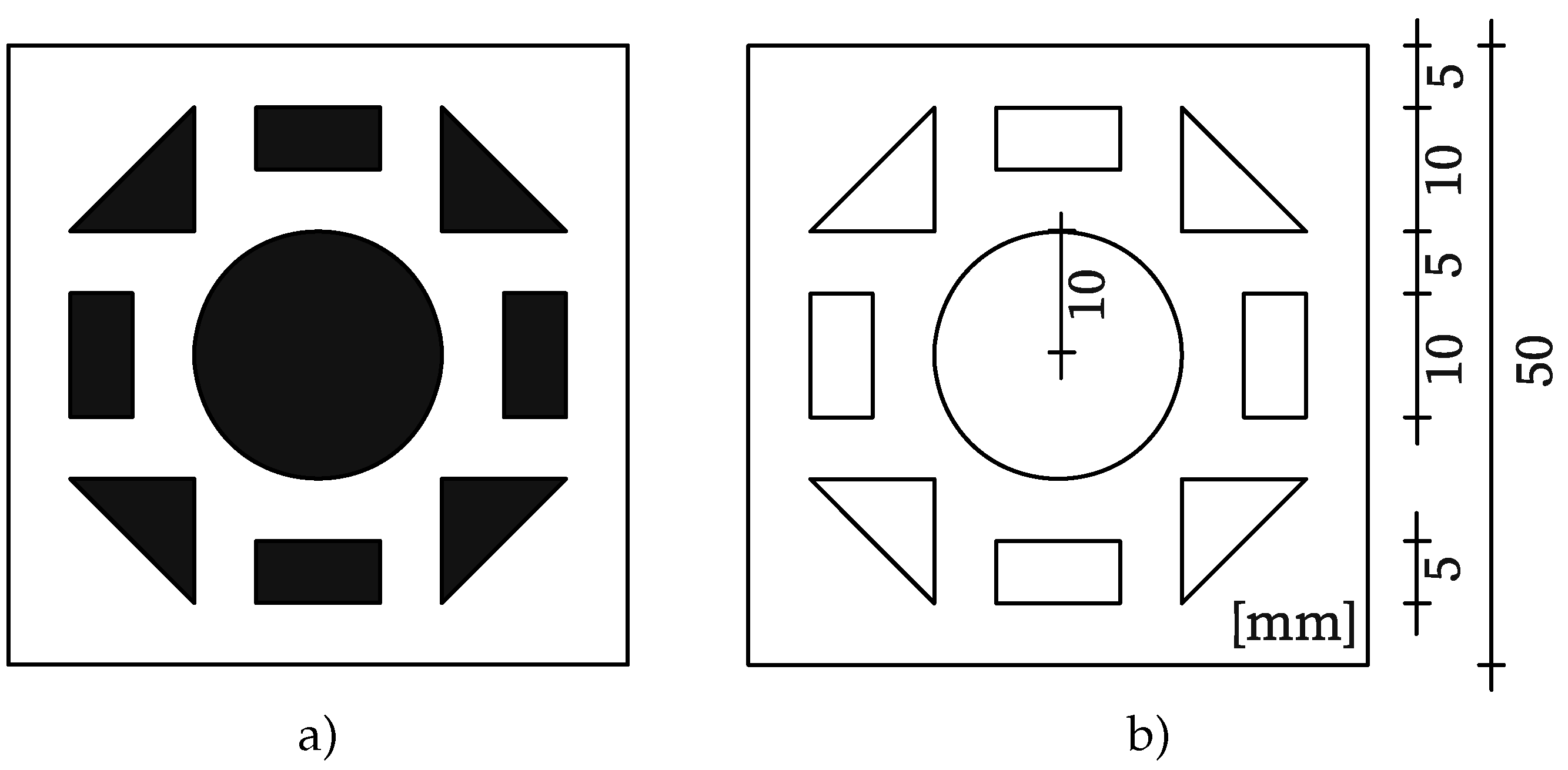
Figure 3.
Schematic test setup.
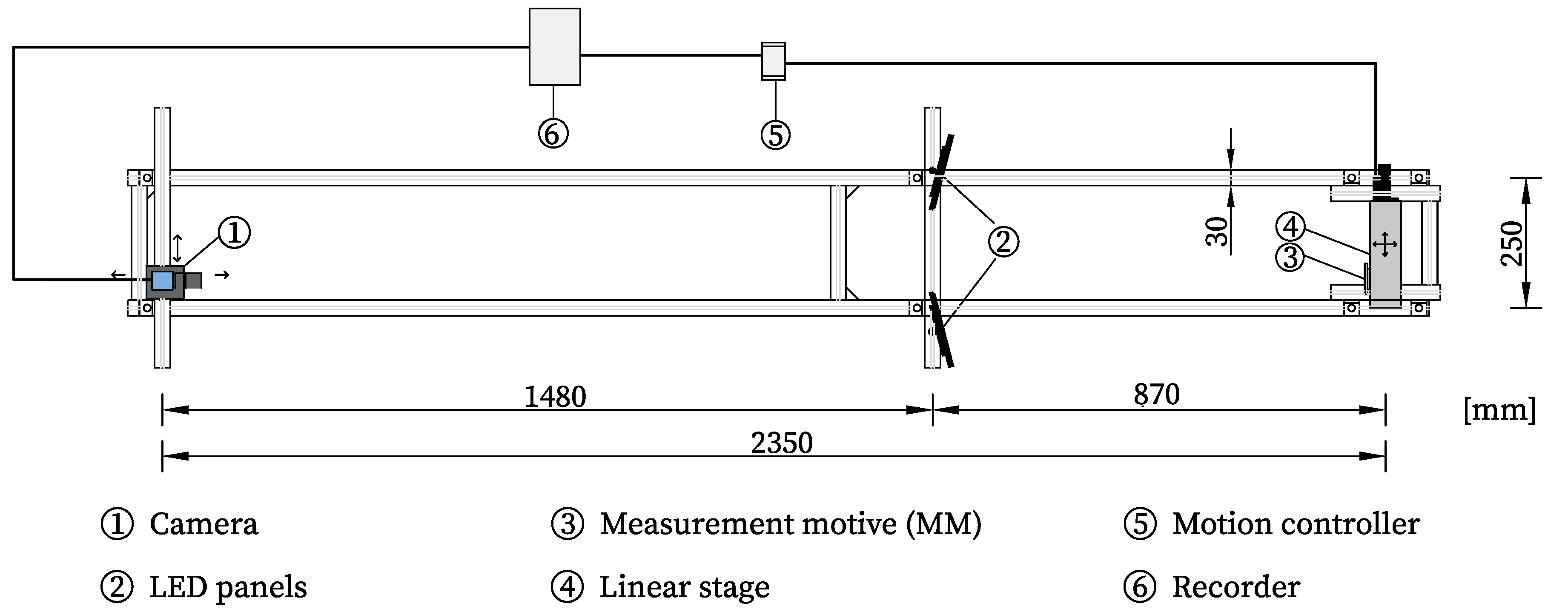
Figure 4.
Displacement path.
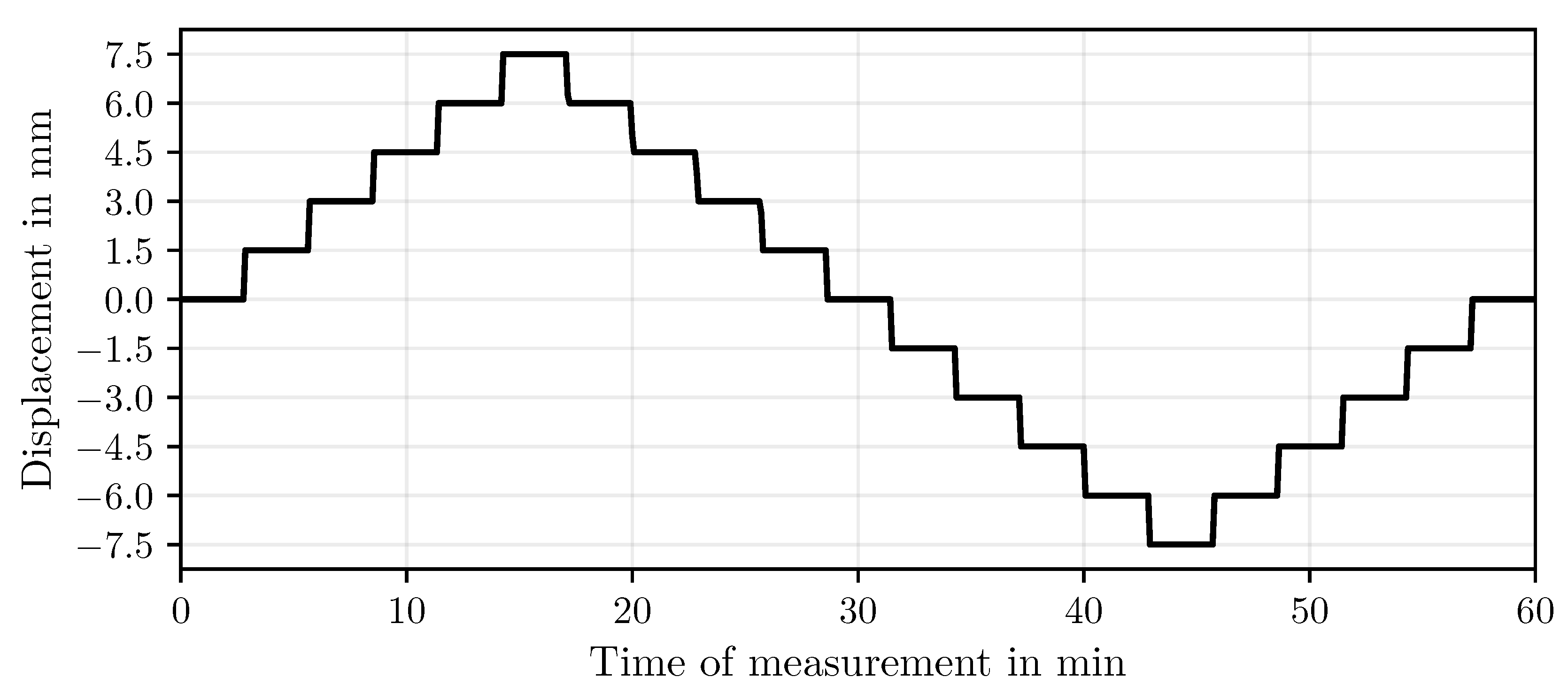
Figure 5.
Confidence scores of YOLO object detection across the dataset.
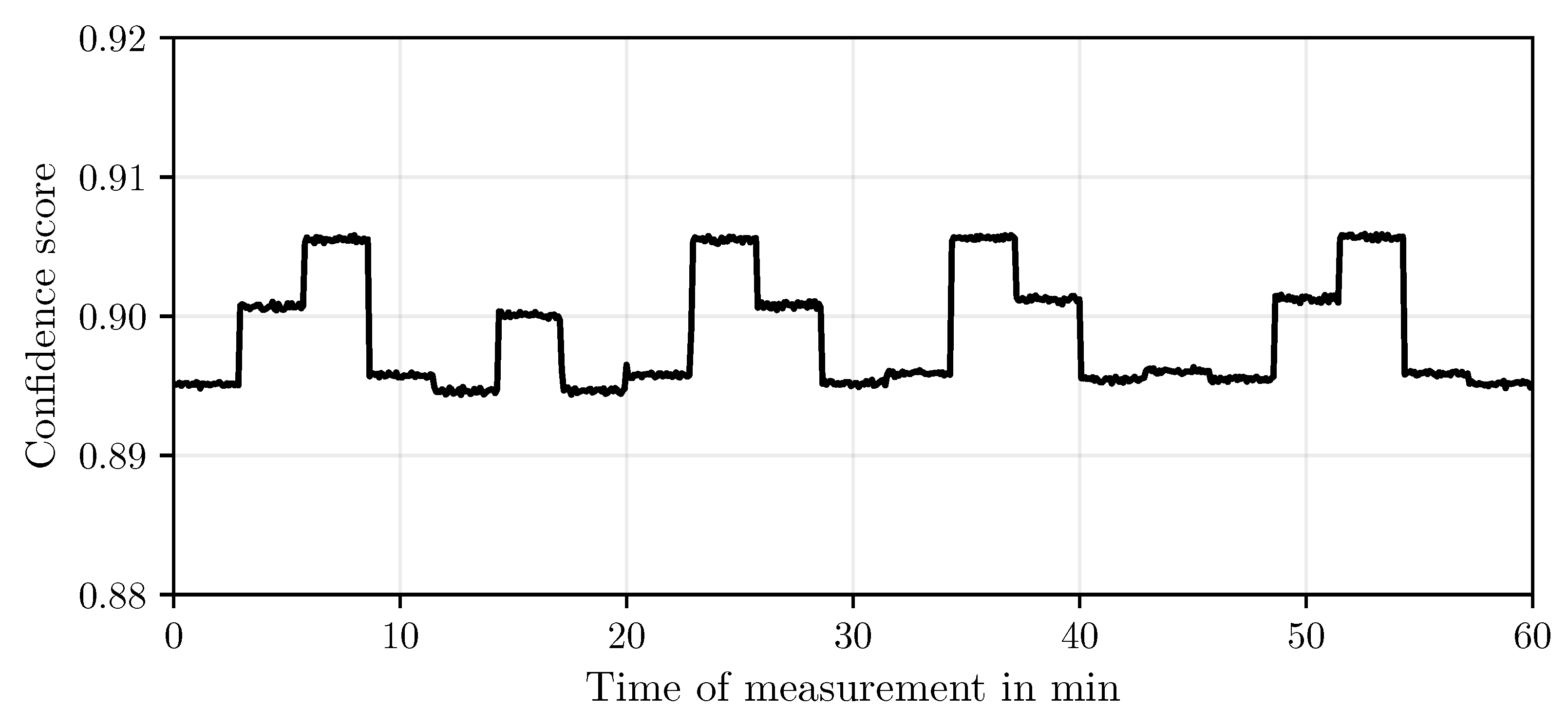
Figure 6.
ROI of the detected MM with applied edge detection.
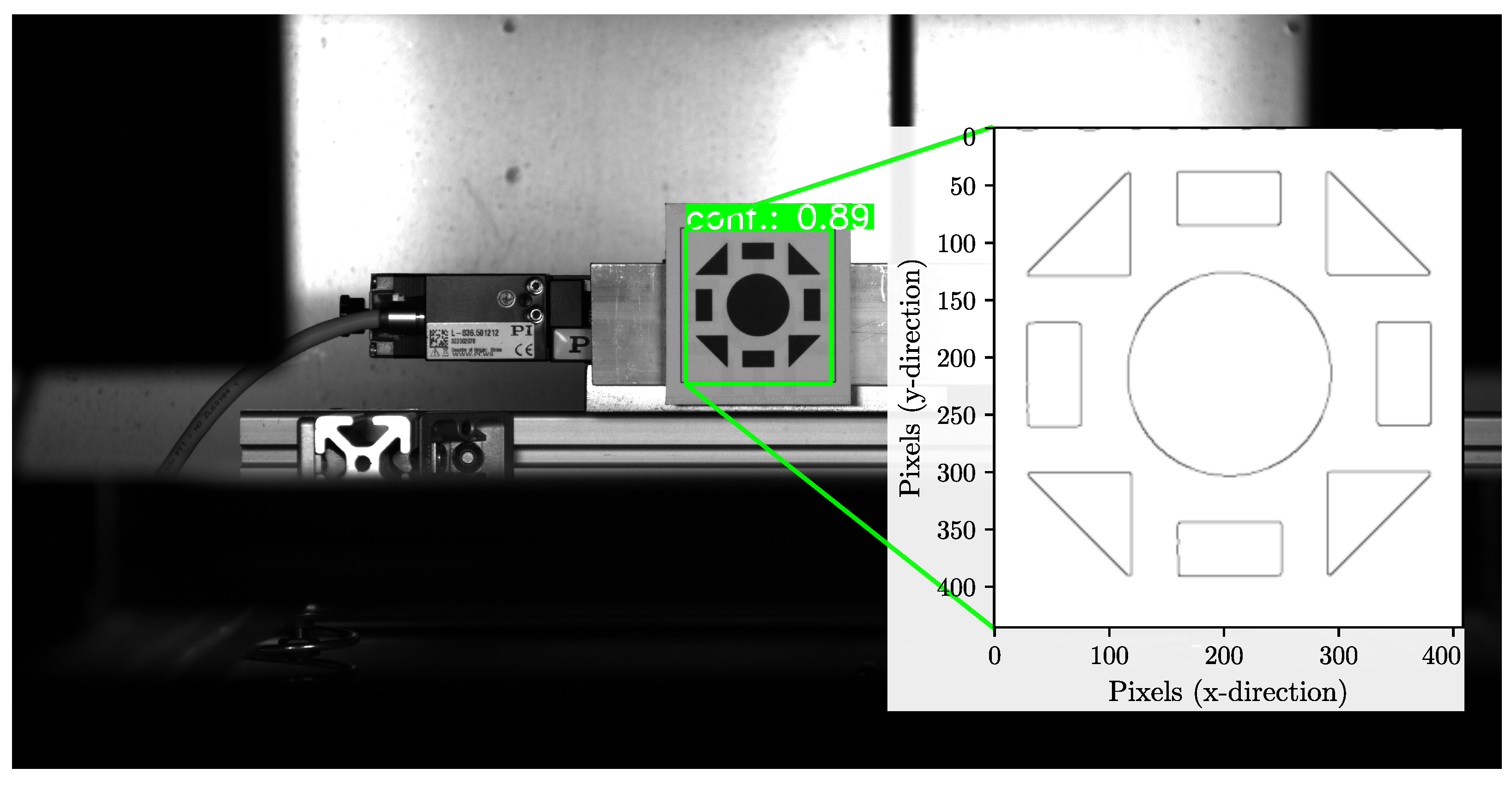
Figure 7.
Segmentation of geometric elements within the MM.
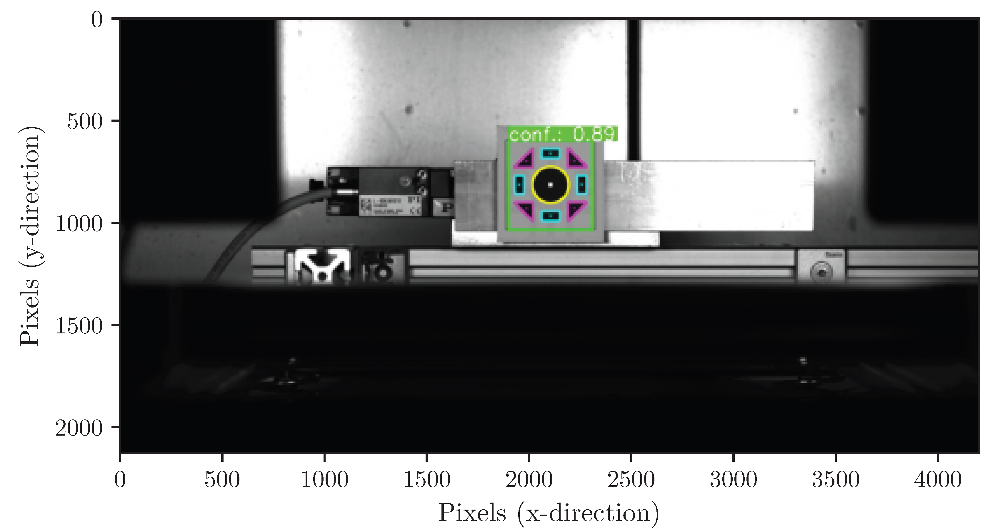
Figure 8.
Centroids of the geometric shapes in the cropped ROI.
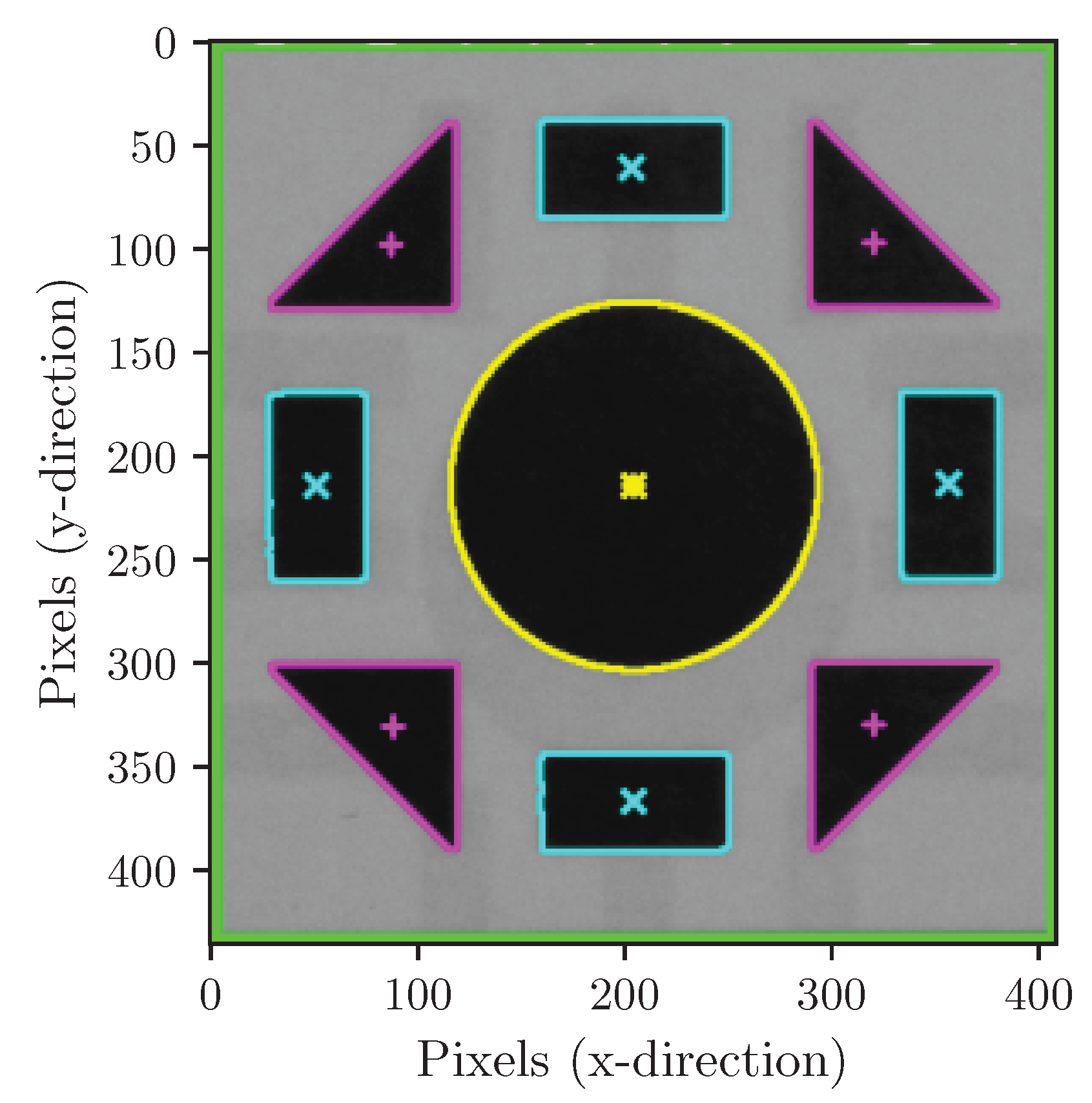
Figure 9.
Comparison of absolute centroid positions for each shape category.
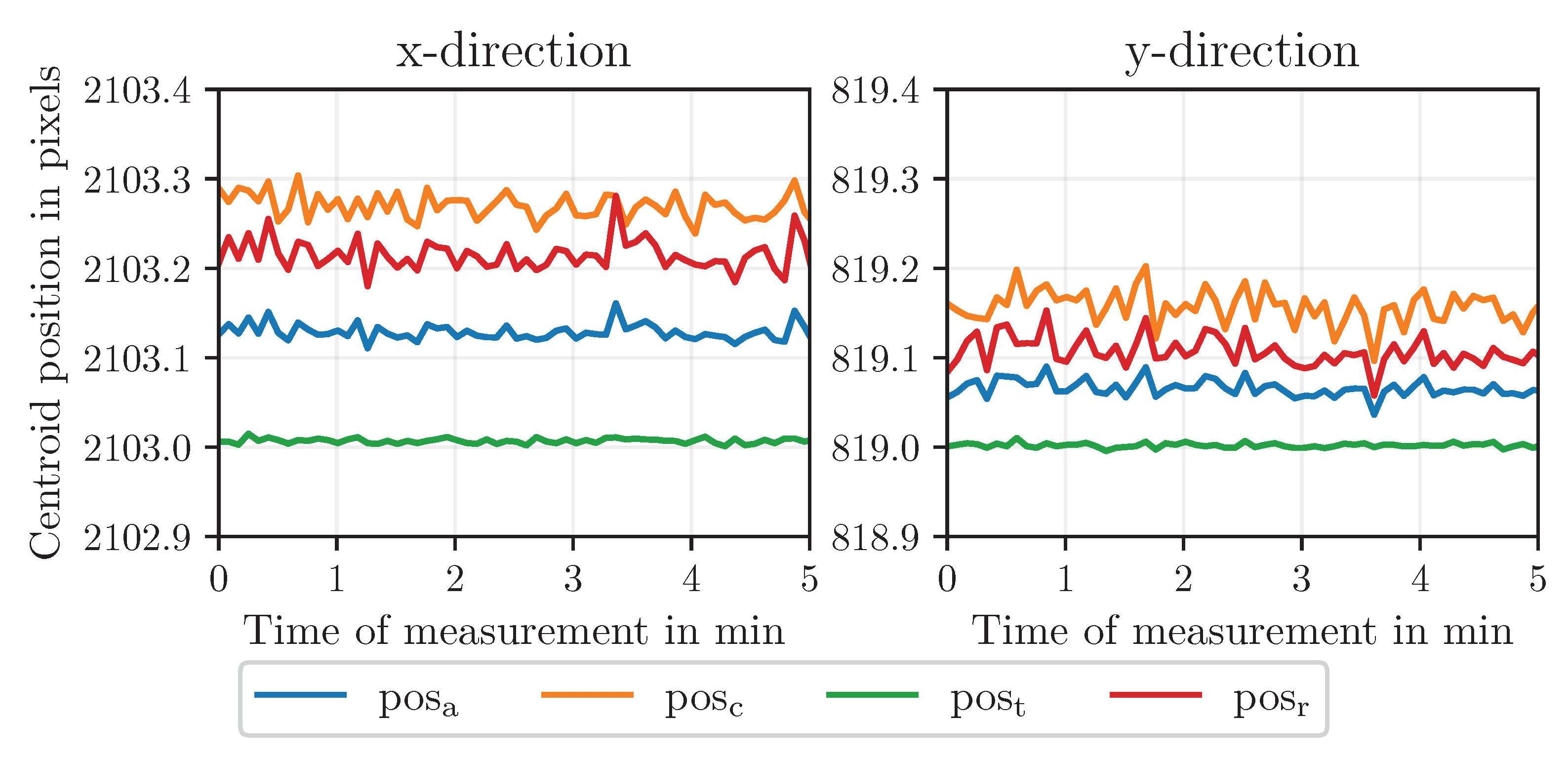
Figure 10.
Image scale values obtained from different geometric elements.
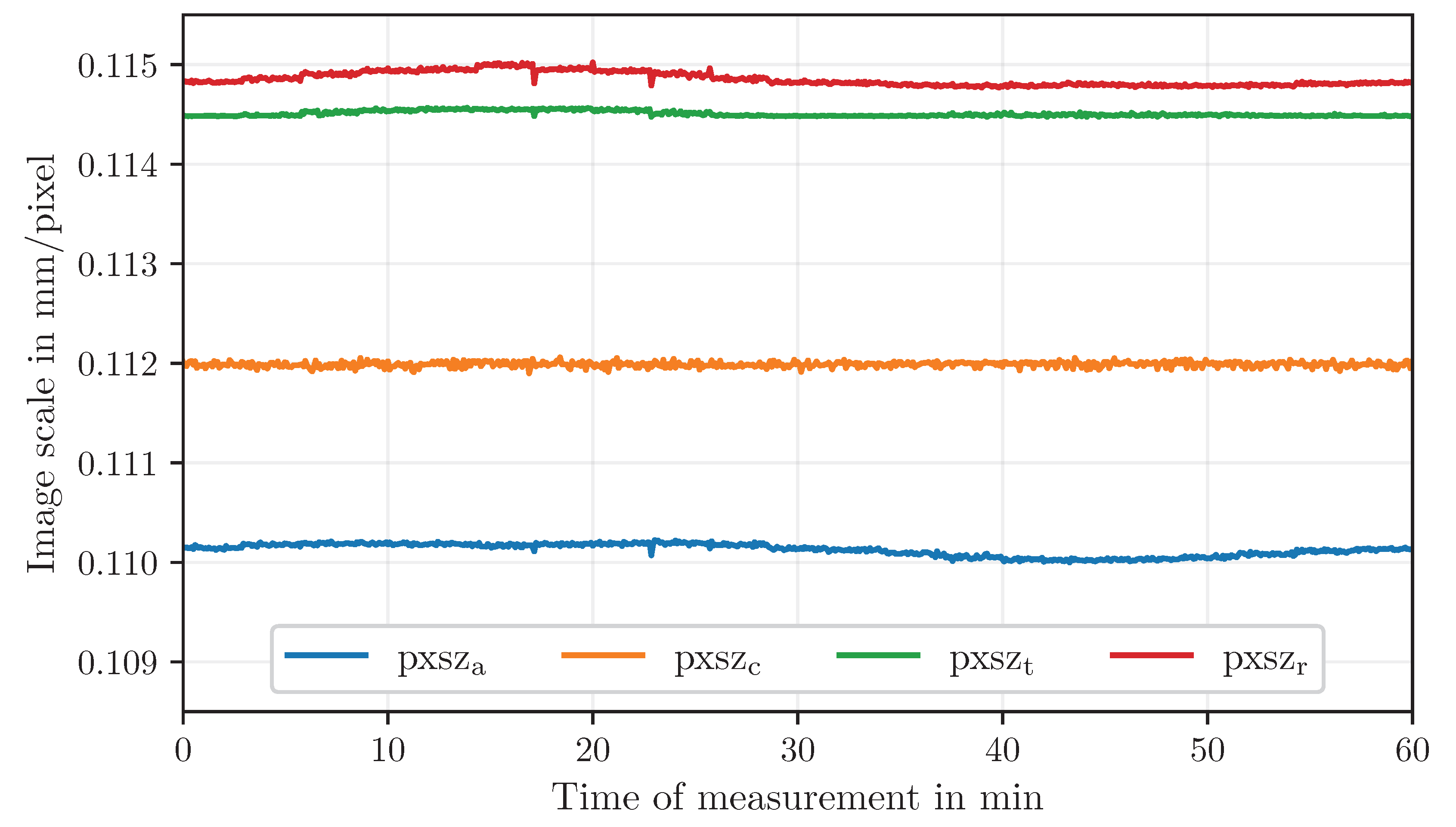
Figure 11.
Comparison of displacement calculation using different methods.
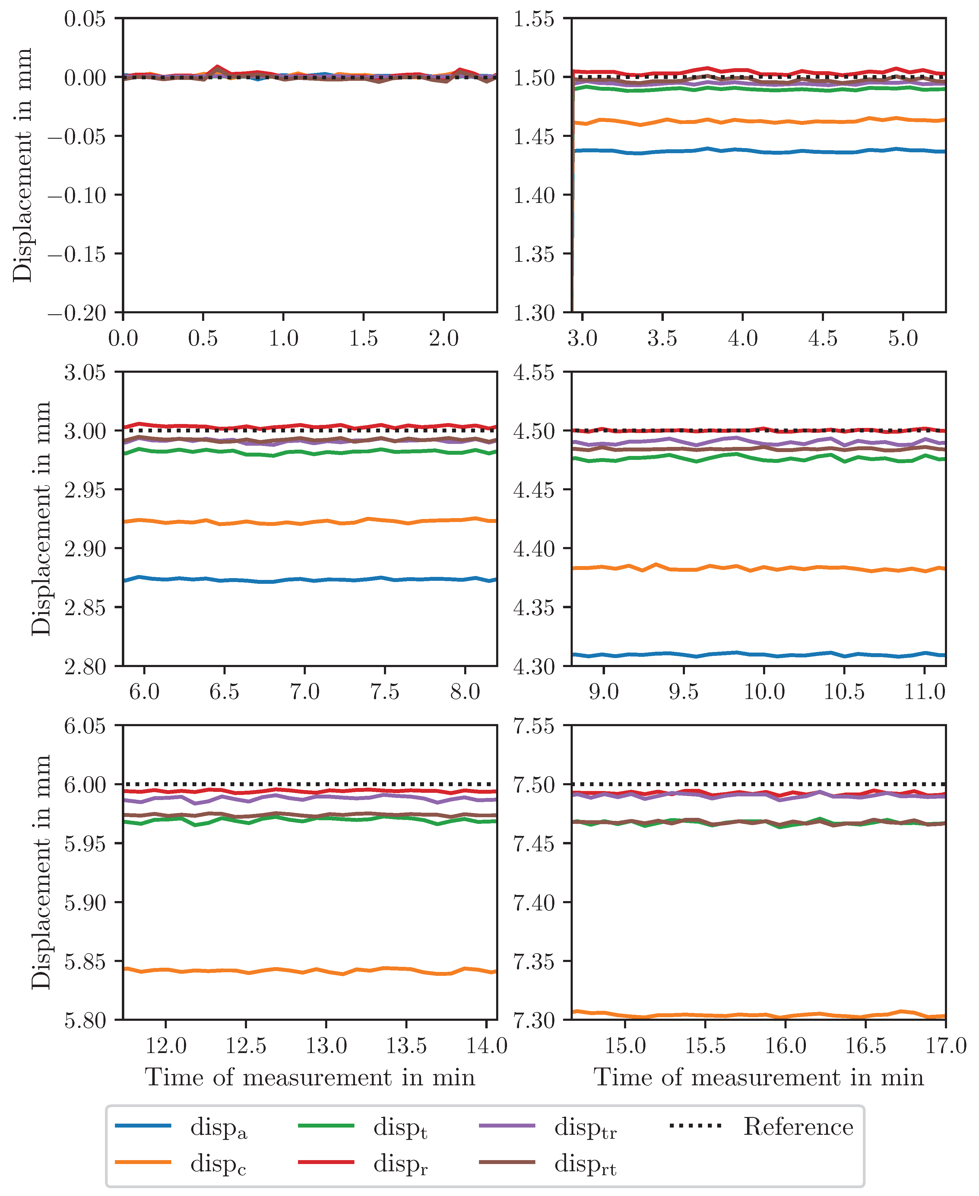
Figure 12.
Absolute deviations of the measurements determined using rectangles.
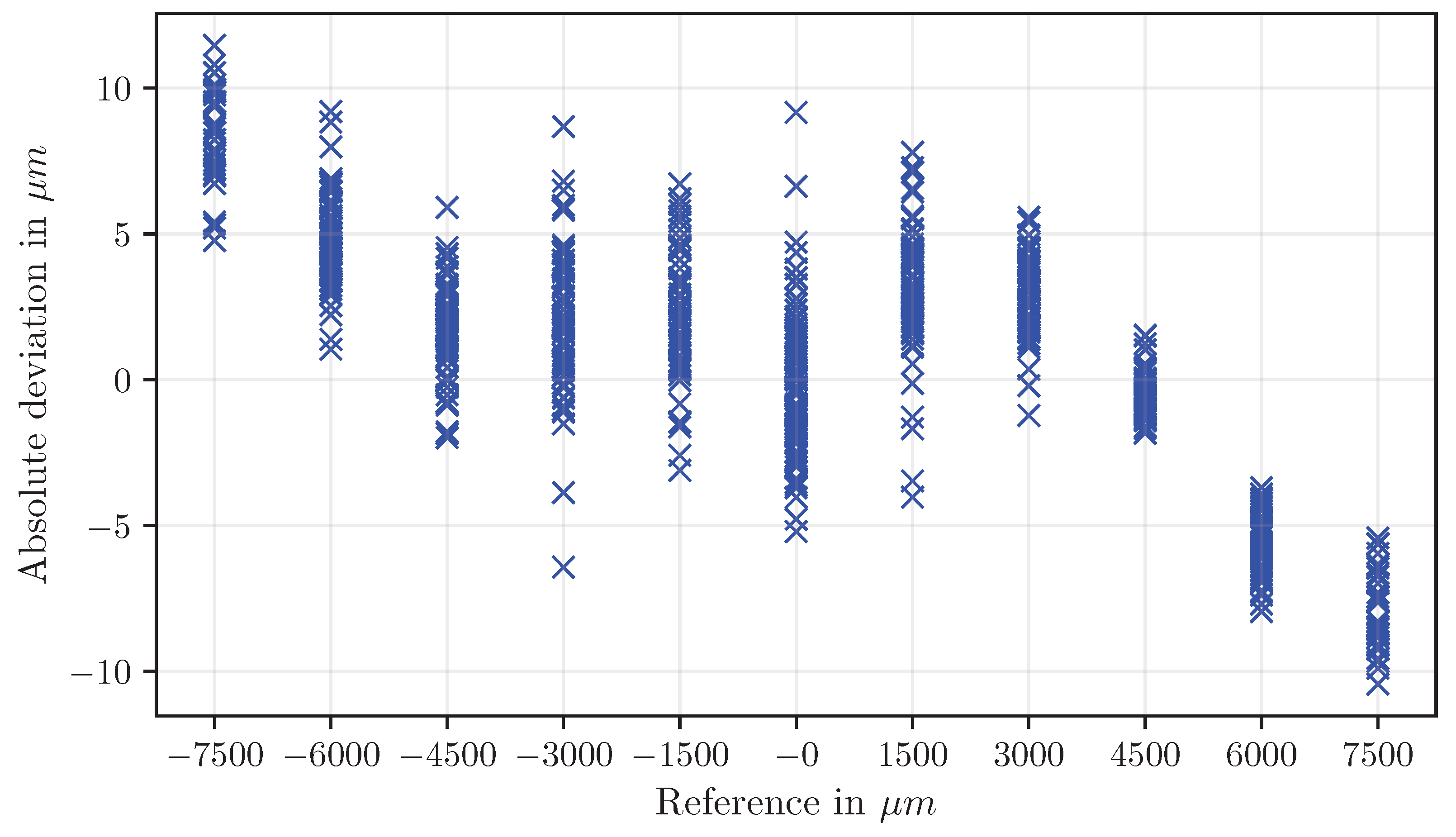
Figure 13.
Measurement uncertainty of the values determined using rectangles.
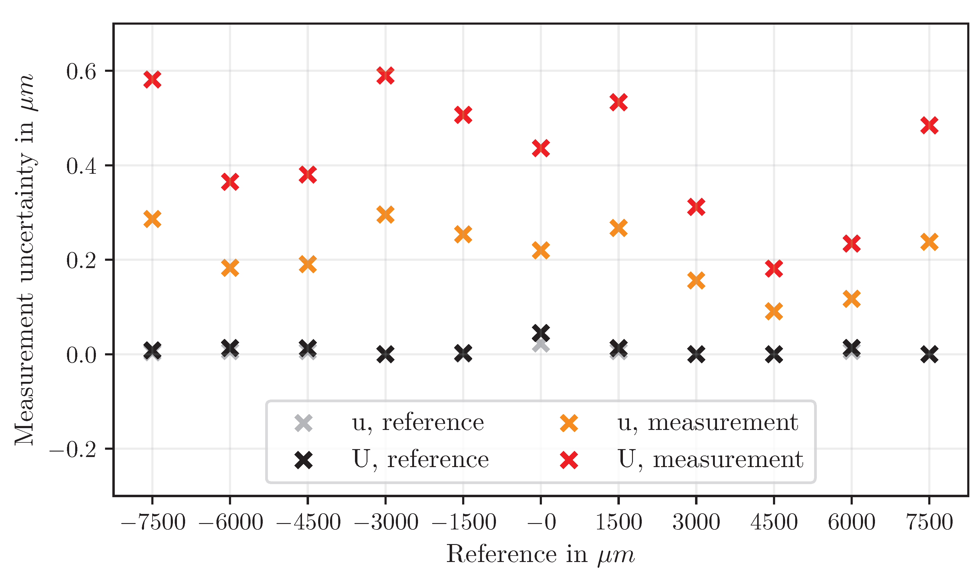
Figure 14.
Absolute deviations of the measurements determined using triangles.
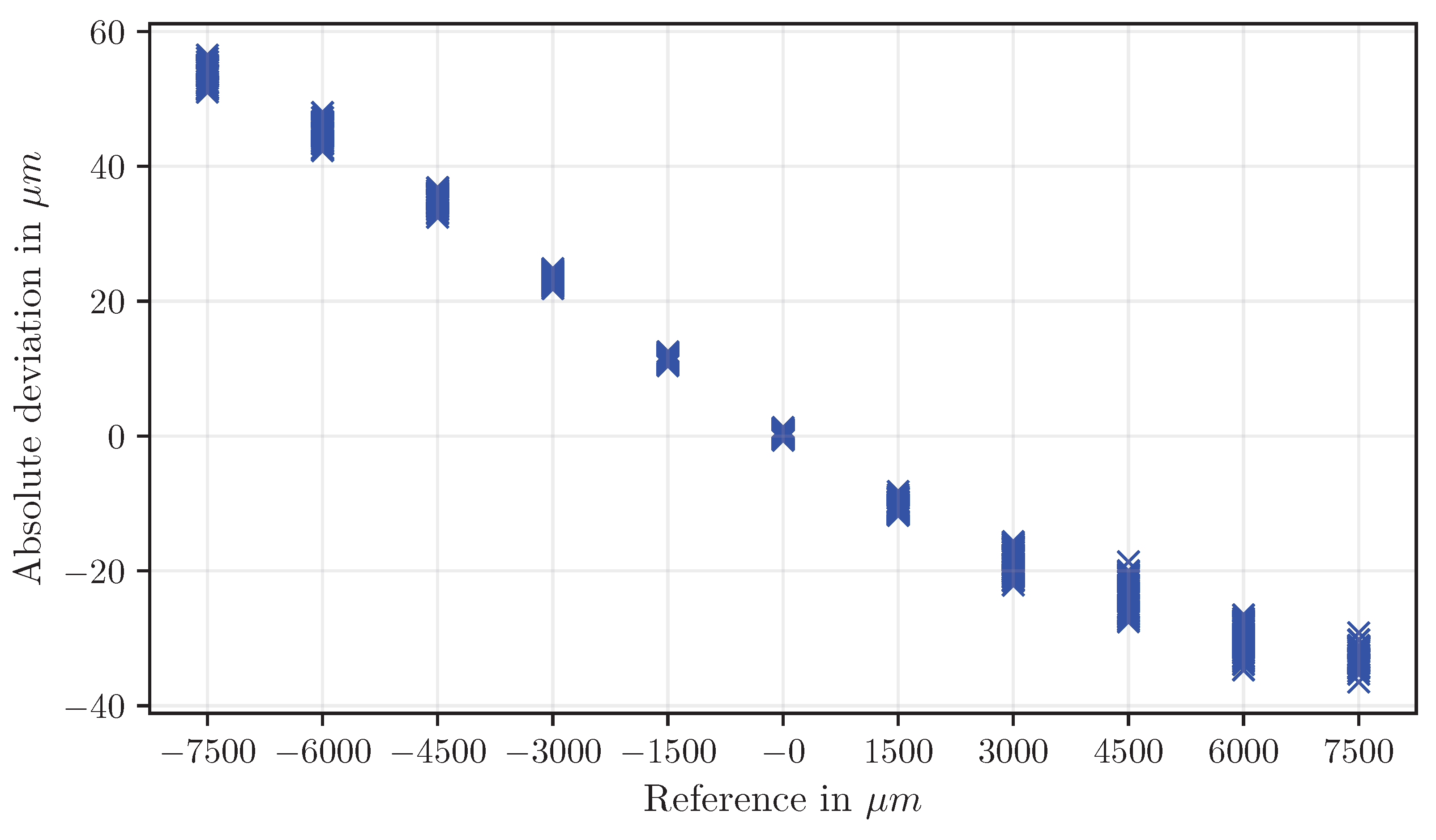
Figure 15.
Measurement uncertainty of the values determined using triangles.
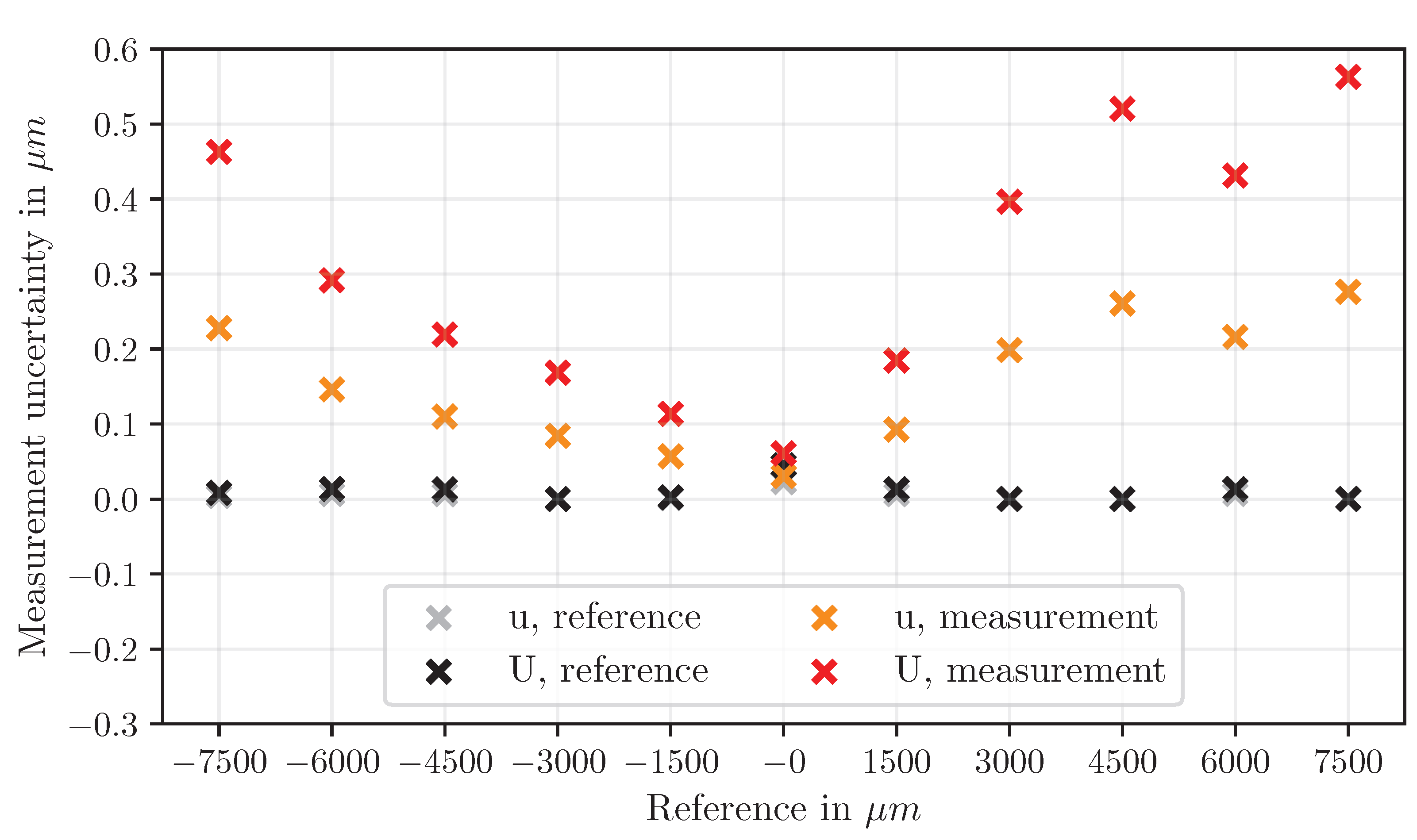
Figure 16.
Absolute deviation of measurements determined using triangles for position and rectangles for image scale (disptr).
Figure 16.
Absolute deviation of measurements determined using triangles for position and rectangles for image scale (disptr).
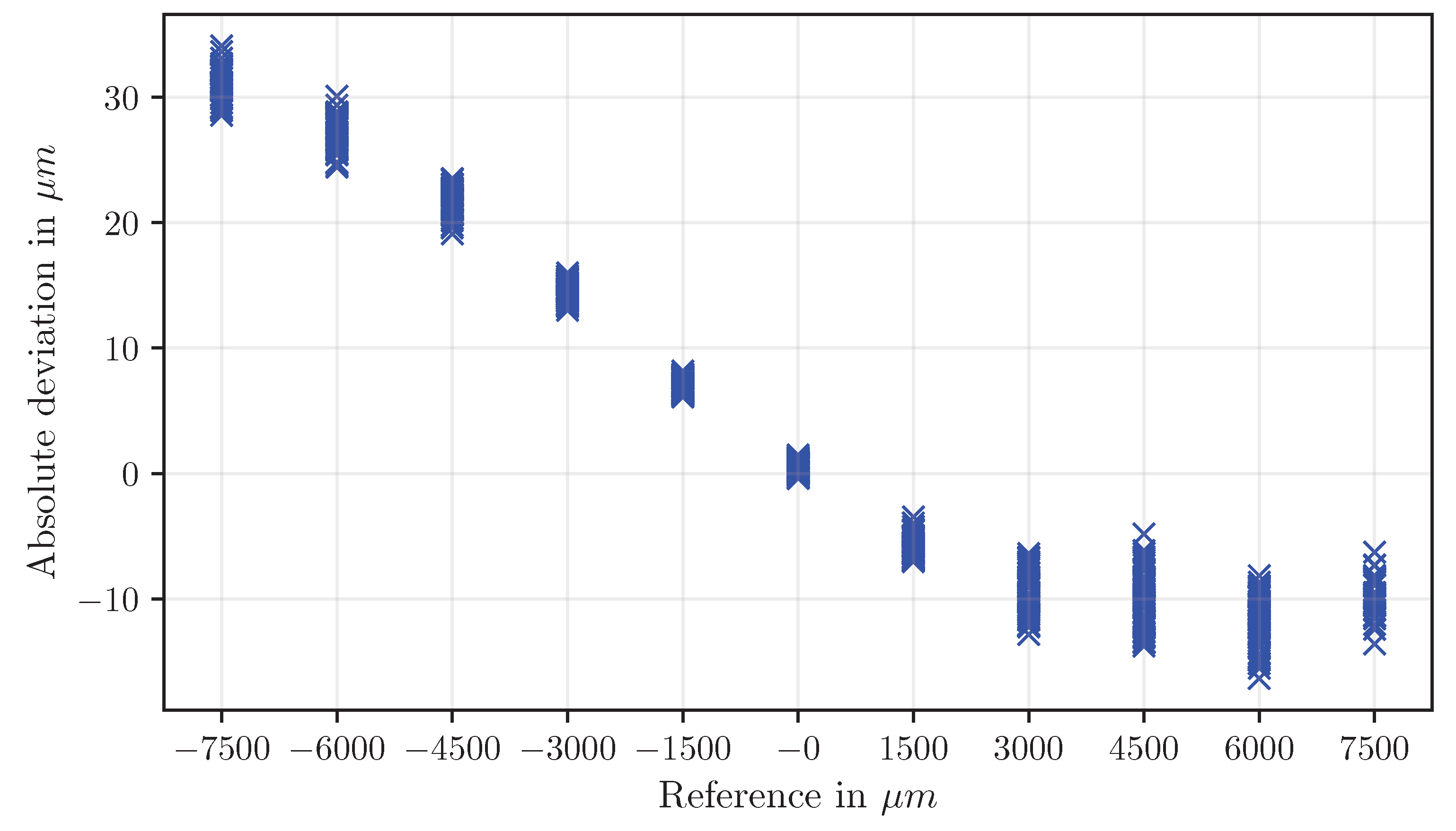
Figure 17.
Measurement uncertainty of measurements determined using triangles for position and rectangles for image scale (disptr).
Figure 17.
Measurement uncertainty of measurements determined using triangles for position and rectangles for image scale (disptr).
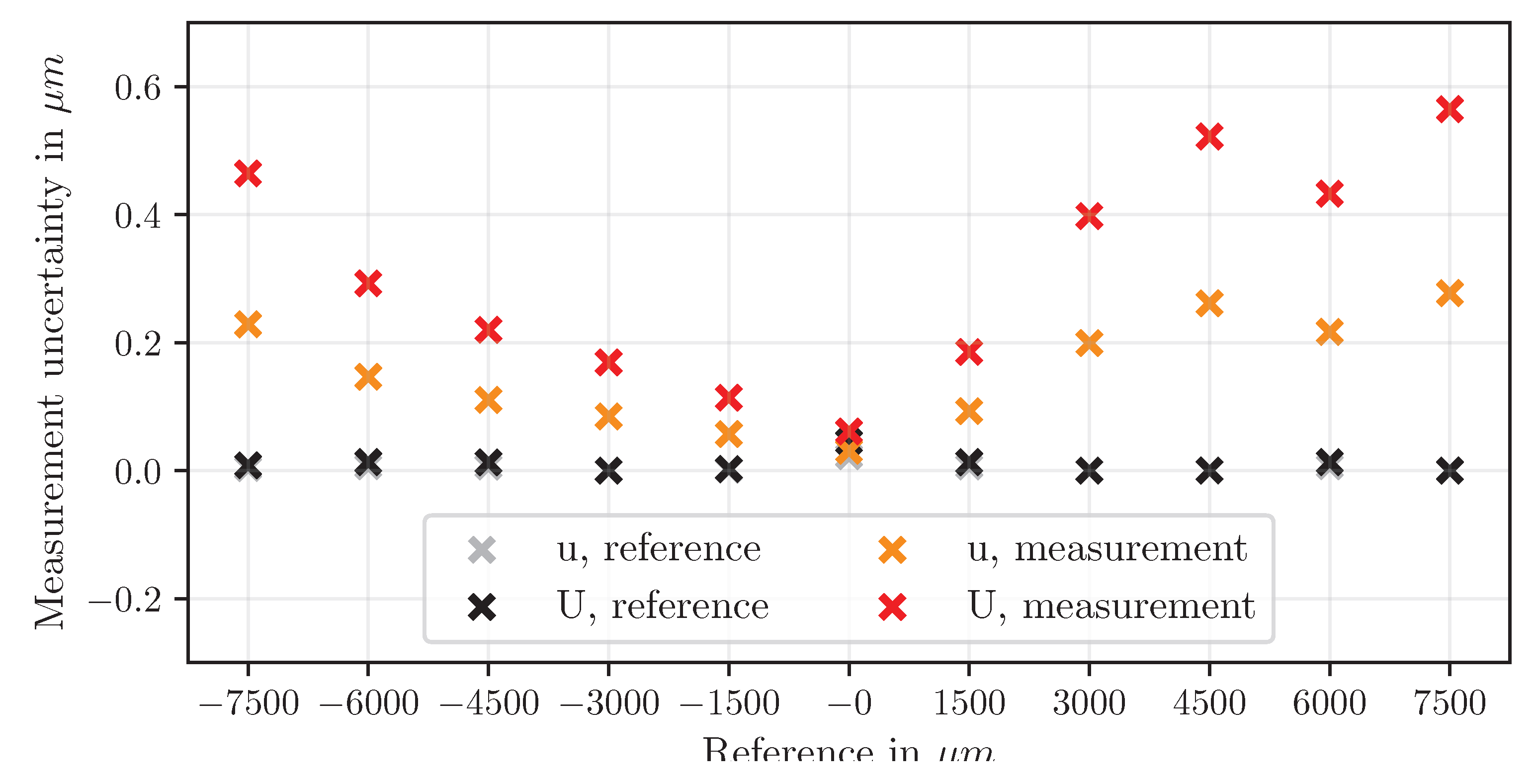
Figure 18.
Absolute deviation of measurements determined using rectangles for position and triangles for image scale (disprt).
Figure 18.
Absolute deviation of measurements determined using rectangles for position and triangles for image scale (disprt).
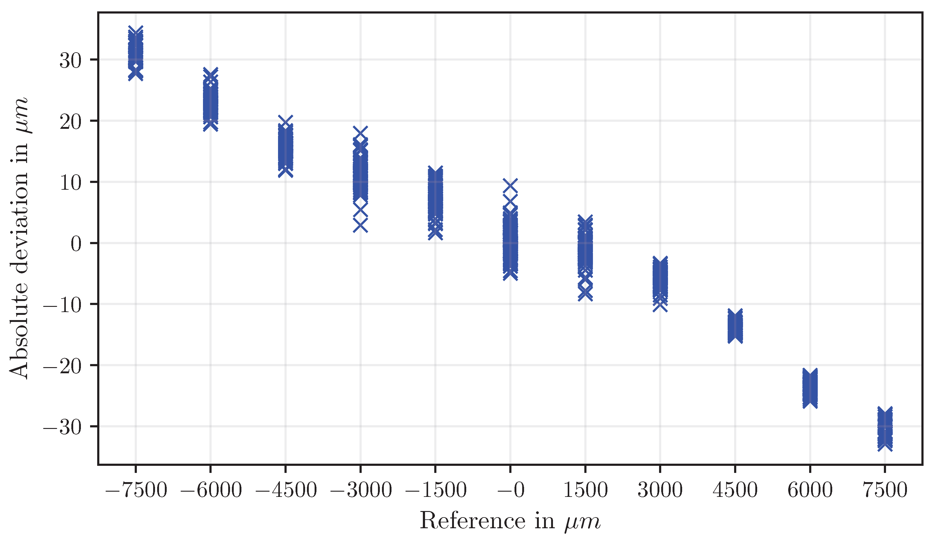
Figure 19.
Measurement uncertainty of measurements determined using rectangles for position and triangles for image scale (disprt).
Figure 19.
Measurement uncertainty of measurements determined using rectangles for position and triangles for image scale (disprt).
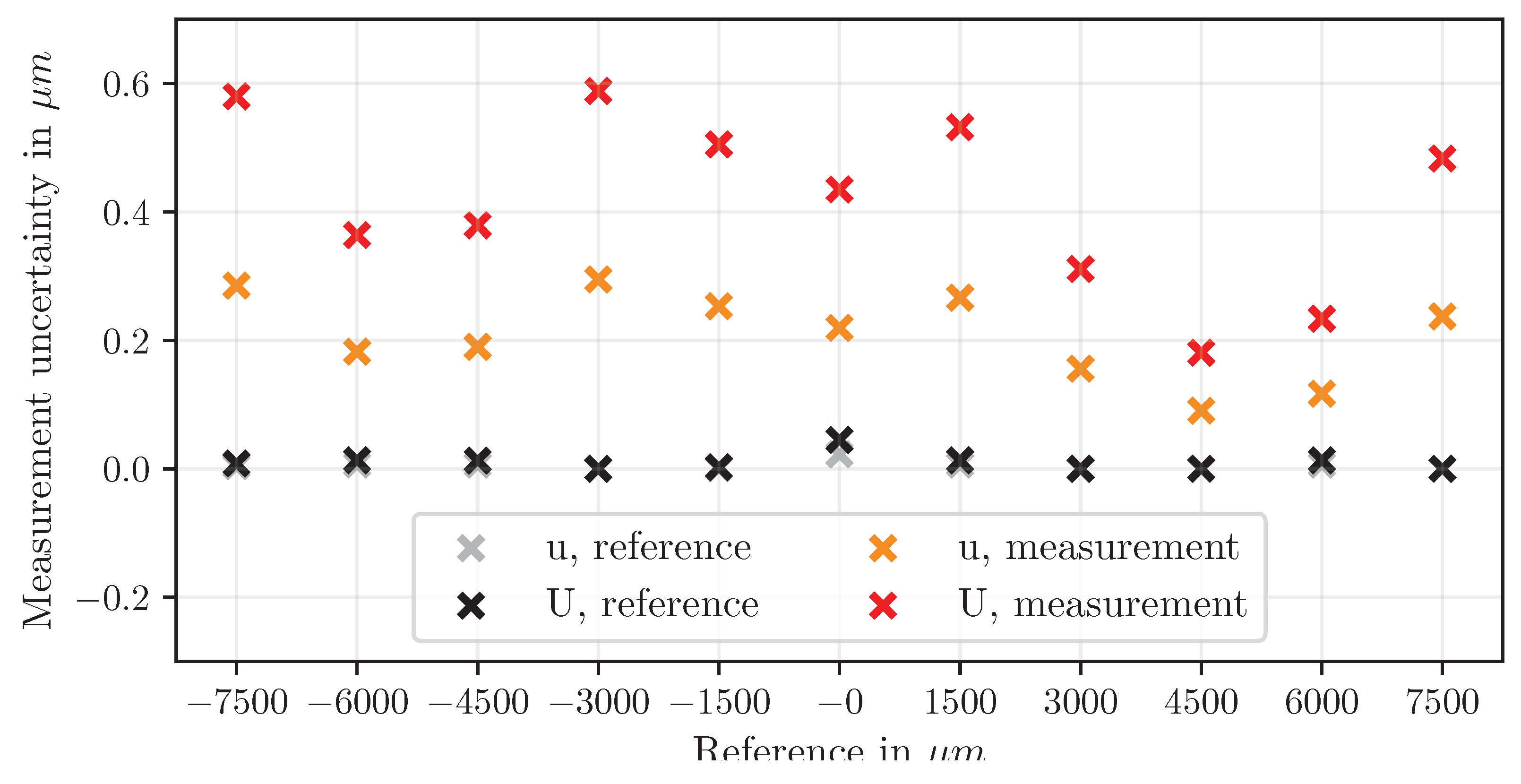
Figure 20.
Absolute deviation of measurements: Approaches based on polygons.
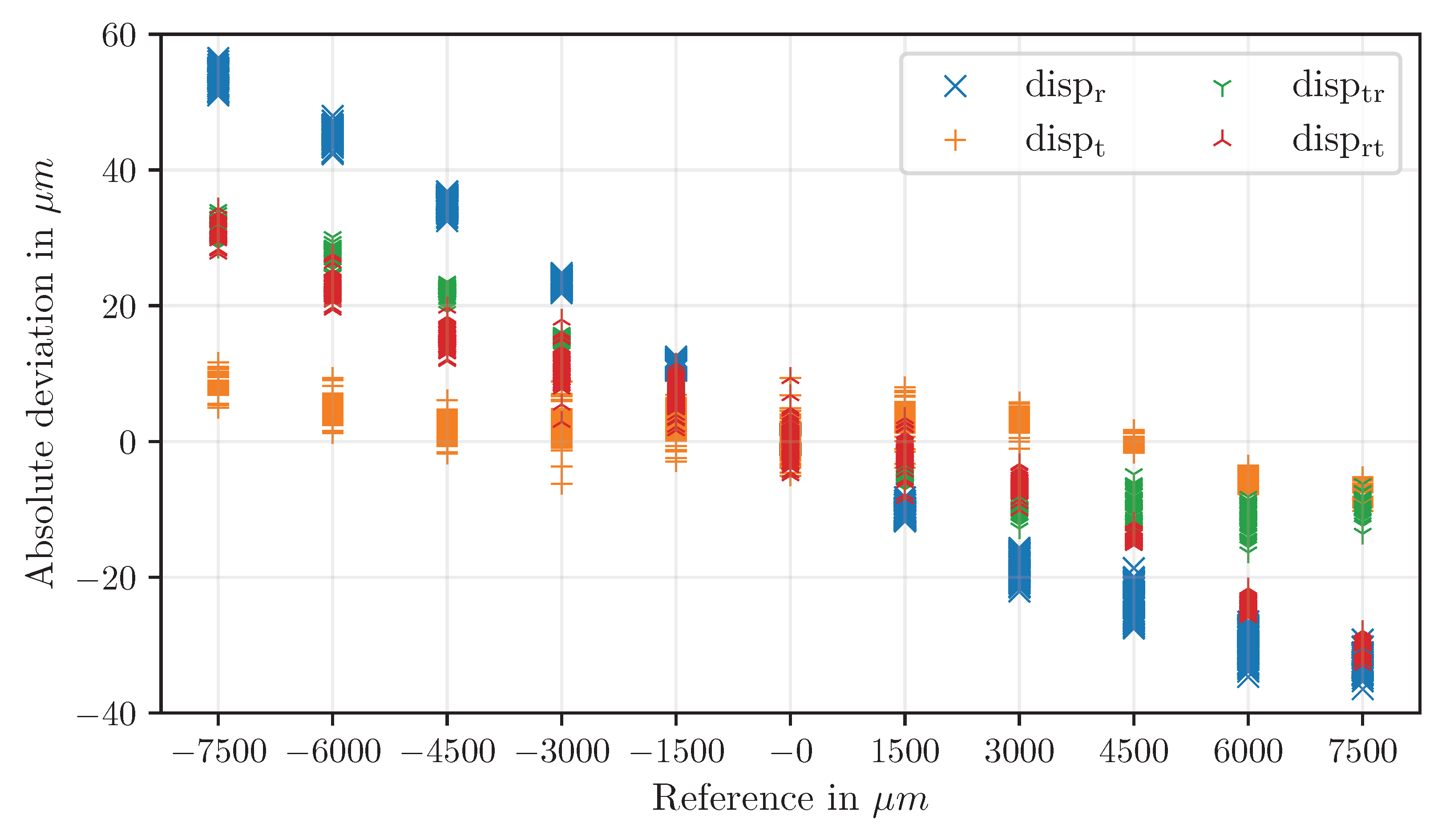

Table 1.
Nomenclature for position determination approaches.
| Abbreviation | Description |
| pos_a | Arithmetic mean of all shape centroids |
| pos_c | Centroid of the circle |
| pos_t | Arithmetic mean of the triangle centroids |
| pos_r | Arithmetic mean of the rectangle centroids |
Table 2.
Nomenclature for image scale determination approaches.
| Abbreviation | Description |
| pxsz_a | Image scale based on the total area of all shapes |
| pxsz_c | Image scale based on the circle radius |
| pxsz_t | Image scale based on distances between triangle centroids |
| pxsz_r | Image scale based on distances between rectangle centroids |
Table 3.
Nomenclature for displacement measurement approaches.
| Abbreviation | Position Determination | Image Scale Calculation |
| dispa | posa | pxsza |
| dispc | posc | pxszc |
| dispt | post | pxszt |
| dispr | posr | pxszr |
| disptr | post | pxszr |
| disprt | posr | pxszt |
Table 4.
Mean values and standard deviations of the image scale determination methods.
| Method | Mean in μm / px | Standard deviation in μm / px |
| pxsza | 0.1101 | 6.1e-5 |
| pxszc | 0.1120 | 2.5e-5 |
| pxszr | 0.1149 | 6.7e-5 |
| pxszt | 0.1145 | 2.6e-5 |
Disclaimer/Publisher’s Note: The statements, opinions and data contained in all publications are solely those of the individual author(s) and contributor(s) and not of MDPI and/or the editor(s). MDPI and/or the editor(s) disclaim responsibility for any injury to people or property resulting from any ideas, methods, instructions or products referred to in the content. |
© 2025 by the authors. Licensee MDPI, Basel, Switzerland. This article is an open access article distributed under the terms and conditions of the Creative Commons Attribution (CC BY) license (http://creativecommons.org/licenses/by/4.0/).
Copyright: This open access article is published under a Creative Commons CC BY 4.0 license, which permit the free download, distribution, and reuse, provided that the author and preprint are cited in any reuse.


