Submitted:
17 June 2025
Posted:
17 June 2025
You are already at the latest version
Abstract
This study investigates trajectory control in flexible manipulators through neural network-based forward and inverse modeling. Traditional improvements in manipulator precision often involve increasing rigidity, which results in greater weight and energy demands—factors that hinder usage in aerospace and other sensitive applications. Flexible manipulators, while lightweight, pose control challenges due to elastic deformations. This research proposes neural network-based models to enhance trajectory control for a two-link, three-degree-of-freedom (3-DOF) flexible manipulator. Simulation and experimental validations demonstrate that compensating for system delays in training data substantially improves tracking accuracy. However, issues with smooth trajectory generation persist. These findings emphasize the utility of neural networks in adaptive control and suggest future avenues for refining input-output modeling to close the gap between theory and implementation.
Keywords:
flexible manipulator
; trajectory control
; neural networks
; forward model
; inverse model
; vibration suppression
; adaptive control
1. Introduction
In the pursuit of enhanced positional accuracy for industrial robotic manipulators, a conventional design strategy has been to increase the structural rigidity of the robot arm. While this approach effectively minimizes deflection and improves tip tracking, it also results in increased mass, higher energy consumption, and greater operational costs. These drawbacks are particularly restrictive in fields such as aerospace, where weight constraints are critical. Additionally, increased rigidity often necessitates larger actuators and structural reinforcements, thereby limiting the robot’s speed and maneuverability [1,6].
To address these limitations, researchers have explored the development of lightweight robotic arms constructed with flexible components. These so-called flexible manipulators, which may consist of single or multiple links, offer several advantages, including reduced energy usage, compact form factors, and the potential for high-speed operation [7,8,9]. The use of smaller actuators and cost-effective materials also lowers manufacturing and maintenance costs, enabling wider applicability in dynamic and constrained environments.
However, the benefits of flexible manipulators are accompanied by significant challenges. The inherent elasticity of the structure introduces vibrations, deformations, and tip oscillations, all of which complicate the control task. These issues are further exacerbated when multiple joints and links are involved, as each additional degree of freedom introduces more dynamic complexity. Extensive research has thus been directed toward vibration suppression and deformation control in flexible manipulators [10,11,12].
Traditional control methods, which assume rigid-body dynamics, struggle to manage the nonlinear and distributed nature of flexible systems. The presence of components such as harmonic drive reducers further complicates control by introducing time delays and residual oscillations during rapid movements. As a result, rigid-body models and conventional inverse kinematics become insufficient for precise trajectory control under these conditions.
To overcome these challenges, researchers have increasingly turned to artificial neural networks (ANNs), which offer powerful nonlinear approximation capabilities. Neural network-based controllers can be broadly categorized into direct methods, such as inverse modeling, and indirect methods, such as adaptive gain tuning [1,4,5,6,7,8,9,10,11,12,13,14,15]. For instance, Gao et al. [10] employed neural networks for vibration suppression and trajectory tracking in a two-link manipulator using the assumed mode method. Abe [11] explored neural networks for flexible Cartesian manipulators, while Sun et al. [12] integrated fuzzy logic into neural models to improve trajectory control. Recurrent neural networks (RNNs) have also been utilized to model forward and inverse dynamics, providing enhanced control via feedforward-feedback loops [13].
Among these studies, Kume et al. [1] demonstrated angle control of a two-link, two-degree-of-freedom flexible manipulator using an inverse model constructed with a hierarchical neural network. While promising, their work was limited to two-dimensional motion and did not extend to full 3D trajectory control—an essential requirement in many modern industrial applications.
This study builds upon and extends prior research by addressing three-dimensional trajectory control of a two-link, three-degree-of-freedom flexible manipulator. We develop both forward and inverse models using neural networks and validate their performance through comprehensive simulations and real-world implementation. Our aim is to bridge the gap between theoretical modeling and practical applicability by incorporating delay-compensated training data and analyzing model behavior under realistic operating conditions.
2. Methods
2.1. Physical Model and Experimental Setup
The experimental platform consisted of a 2-link, 3-degree-of-freedom (3-DOF) flexible manipulator constructed using stainless steel for Link 1 and aluminum for Link 2 as shown in Figure 1a. Each joint was actuated by a DC servo motor equipped with a harmonic drive to achieve high-precision rotational control. Joint 2 and Joint 3 supported angular motion of ±90°, while Joint 3 could additionally perform full 360° rotation. Encoders with 1000 pulses per revolution (P/R) were mounted on each motor shaft, and all joints used harmonic drives with a 1:100 reduction ratio. Cast iron counterweights were added to counterbalance each motor, and a weight was placed at the tip of the arm to induce measurable elastic deformation during movement.
Strain gauges were mounted on the links to measure bending and torsional deformation. The manipulator’s end-effector trajectory was tracked using an OptiTrack optical motion capture system. The physical and mechanical specifications of all components, including actuators, harmonic drives, and structural elements, are detailed in Table 1.
The control system architecture is presented in Figure 1b. Control algorithms were developed in MATLAB Simulink, compiled to C code using Real-Time Workshop (RTW), and deployed to a Digital Signal Processor (DSP) board (DS1003, dSPACE). The DSP communicated with a D/A converter and speed-controlled servo amplifiers (DA2 series, Sanyo Denki) to actuate the motors. Encoder signals were processed via a counter board, while strain gauge voltages were extracted using bridge circuits and amplified using dynamic strain meters (Kyowa Electric DPM713B, DPM913B), and then digitized through an A/D converter. The sampling interval was set to 0.01 seconds.
2.1. Neural Network Training
Neural network training was conducted using an offline learning approach based on the Levenberg–Marquardt (LM) algorithm. This method is widely adopted due to its hybrid optimization mechanism that combines the fast convergence properties of Newton’s method with the stability of gradient descent.
The training objective was to minimize the mean squared error (MSE) between the neural network output and the target values, as defined by the loss function in (1):
or in vector notation as shown in (2):
Let be the Jacobian of , given by (3):
2.1.1. Gradient Descent Approach
The steepest descent method approximates the minimum of the objective function using the gradient. The gradient vector of the objective function is expressed as (4).
The weight update rule becomes (5).
where is the learning rate. However, as a first-order method, steepest descent exhibits slow convergence.
2.1.2. Newton’s Method
Newton’s method enhances convergence using a second-order approximation. The Hessian of the objective function is given by (6).
Neglecting second-order residuals, can be approximated to 0, and the Hessian matrix can be approximated as (7).
Therefore, the update equation for Newton’s method can be expressed as (8).
While this provides fast convergence, it requires that is positive definite. If not, the update direction may increase the loss function, leading to instability.
2.1.3. Levenberg–Marquardt Method
The LM method addresses this by interpolating between steepest descent and Newton’s method. The weight update rule is defined as (9).
where is the damping factor, When μ→0, the method approaches Newton’s method; for large μ, it behaves like gradient descent. The value of μ is adapted dynamically: it is decreased when the error decreases and increased when the error rises, allowing for both robustness and fast convergence.
Training was conducted offline, where data was collected over time and processed in batch mode. This contrasts with online learning, where updates are made in real time for each new sample. Offline training is particularly effective for systems exhibiting periodic behaviors, such as cyclic robot motions.
2.1.4. Neural Network Architecture
The neural network employed in this study consisted of 11 layers: one input layer, ten hidden layers, and one output layer. Sigmoid activation functions were used for the input and hidden layers, enabling nonlinear mapping, while a linear activation function was applied to the output layer to ensure smooth signal generation.
The learning dataset comprised pairs of inverse kinematics joint angles and corresponding measured trajectories. This setup formed the basis for a direct inverse model, where the network maps desired end-effector positions to the required motor input angles.
Training used the LM algorithm as described, with a mean squared error cost function. The damping factor μμ was dynamically adjusted with an increment factor of 0.1 and a decrement factor of 10, optimizing the learning process to avoid overfitting and poor convergence.
2.2. Verification of Control
To evaluate the control system’s performance, a circular trajectory was prescribed for the flexible manipulator using inverse kinematics. The control experiment was carried out under a proportional (P) control scheme. The results were analyzed to assess tracking accuracy and dynamic response under realistic conditions. The experimental configuration used for this test is shown in Figure 2, which illustrates the control flow from the target trajectory input to the output response of the flexible manipulator.
The comparison between target and measured data is presented in Figure 3. From Figure 3a, it is evident that the motor output angle lags behind the reference angle computed via inverse kinematics. This delay is primarily attributed to the compliance of the harmonic drive, which introduces elastic behavior in the joint transmission.
Figure 3b further reveals that the output trajectory of the arm tip is delayed by approximately 0.3 seconds relative to the target trajectory. This phase lag is considered to stem from the mechanical flexibility of the links and transmissions. Specifically, the time delay is caused by the propagation of movement from the motor base through the flexible links to the tip of the manipulator. As a result, the end-effector trajectory fails to synchronize with the ideal path in real time.
In Figure 3c, additional steady-state deviation is observed: the trajectory shifts toward the negative Y-axis and the positive Z-axis. This positional offset is likely due to a combination of physical asymmetries in the hardware and the limitations of using P control alone. The absence of integral or derivative components in the controller means that steady-state errors are not actively corrected during operation.
These observations underscore two key findings:
- Time-delay effects introduced by mechanical flexibility significantly impact tracking accuracy.
- Steady-state offsets arise from uncompensated structural and control limitations, especially when using minimal control schemes.
This verification step confirms that the experimental setup exhibits notable dynamic lag and spatial deviation, which must be considered when training the neural network models for improved trajectory prediction and control fidelity.
2.3. Neural Network Experiment Setup
A forward model and an inverse model were constructed using the inverse kinematics output angle and the actual output trajectory in Figure 4. The input and output data used for training the neural network are shown in Figure 4a. The training data was randomly divided into training data, validation data, and test data, with the ratios set to 70/100, 15/100, and 15/100. The training data was used for training the neural network. The validation data was used to improve generalization, and the number of consecutive increases in the mean square error of the validation data was limited to terminate the learning before overfitting occurred. The test data was used only to evaluate the performance of the neural network after training, independent of the learning.
The learning termination conditions are shown in Table 2. In addition, the increase coefficient of the weight μ in the Levenberg-Marquardt method update formula was set to 0.1, and the decrease coefficient was set to 10.
3. Results and Discussion
Neural networks were trained using data sets that included target and actual trajectories, divided into training, validation, and test subsets. Results showed that while the forward model successfully predicted output trajectories, the inverse model struggled due to a phase shift caused by system delays.
3.1. Training Performance of the Neural Network
The training results for the forward and inverse neural network models are summarized in Figure 5. The stopping criterion for both models was set as 1000 consecutive increases in the validation error to prevent overfitting. Training concluded after 1030 iterations for the forward model and 2088 iterations for the inverse model, as outlined by the learning termination conditions.
As shown in Figure 5a, the output angle generated by the inverse model closely aligns with the angle computed through inverse kinematics. This agreement verifies that the inverse model successfully learned the underlying input-output relationship.
In Figure 5b, the forward model’s predicted trajectory closely tracks the target trajectory; however, slight deviations are observed around 0 and 5 seconds. These deviations are likely due to inconsistencies between the trajectory at the beginning of the circular motion and during the second revolution. The variations stem from physical effects in the actual hardware, such as flexural settling, which the neural network attempted to reconcile during learning.
As illustrated in Figure 6a,b, both the output angle of the inverse model and the forward model’s generated trajectory showed notable discrepancies from the desired inverse kinematics angles and target path. Specifically, the output trajectory deviated significantly from a perfect circular orbit, indicating residual modeling inaccuracies.
Nonetheless, consistent waveform patterns were observed: the Y-direction motion correlated strongly with the response of Joint 1, and the Z-direction motion was closely linked to Joint 3. These correlations suggest that while the network captured some key relationships between joint actuation and spatial motion, the dynamic behavior under real conditions remains challenging to model precisely.
3.3. Results of Delay Compensation Through Adjusted Training Data
To address the identified delay, training datasets were adjusted by advancing the actual output trajectory relative to the inverse kinematics angles by 0.28 s, 0.29 s, and 0.30 s. Simulation results for each case are shown in Figure 7, with the associated mean squared errors listed in Table 3.
Results showed that 0.29 s produced the lowest error and the closest visual match to the target trajectory. Therefore, 0.29 s was selected as the optimal lead for aligning training data.
Simulations using models trained on the 0.29 s adjusted data demonstrated enhanced tracking performance compared to the original unadjusted models. The inverse model output angle more closely approximated inverse kinematics results but still lacked full continuity. The forward model continued to reflect accurate directional mapping between joints and tip motion.
To explain the residual deviation, wave propagation speeds within the manipulator links were calculated using elasticity theory:
Torsional velocity
Bending velocity: , where
Estimated propagation duration for joint 1, 2 and 3 based on material and geometric properties were 0.000175 s, 0.109 s and 0.073 s respectively. These values confirm that delays differ per joint, suggesting that future learning datasets may benefit from per-joint temporal alignment.
3.4. Implementation Experiment and Physical Validation
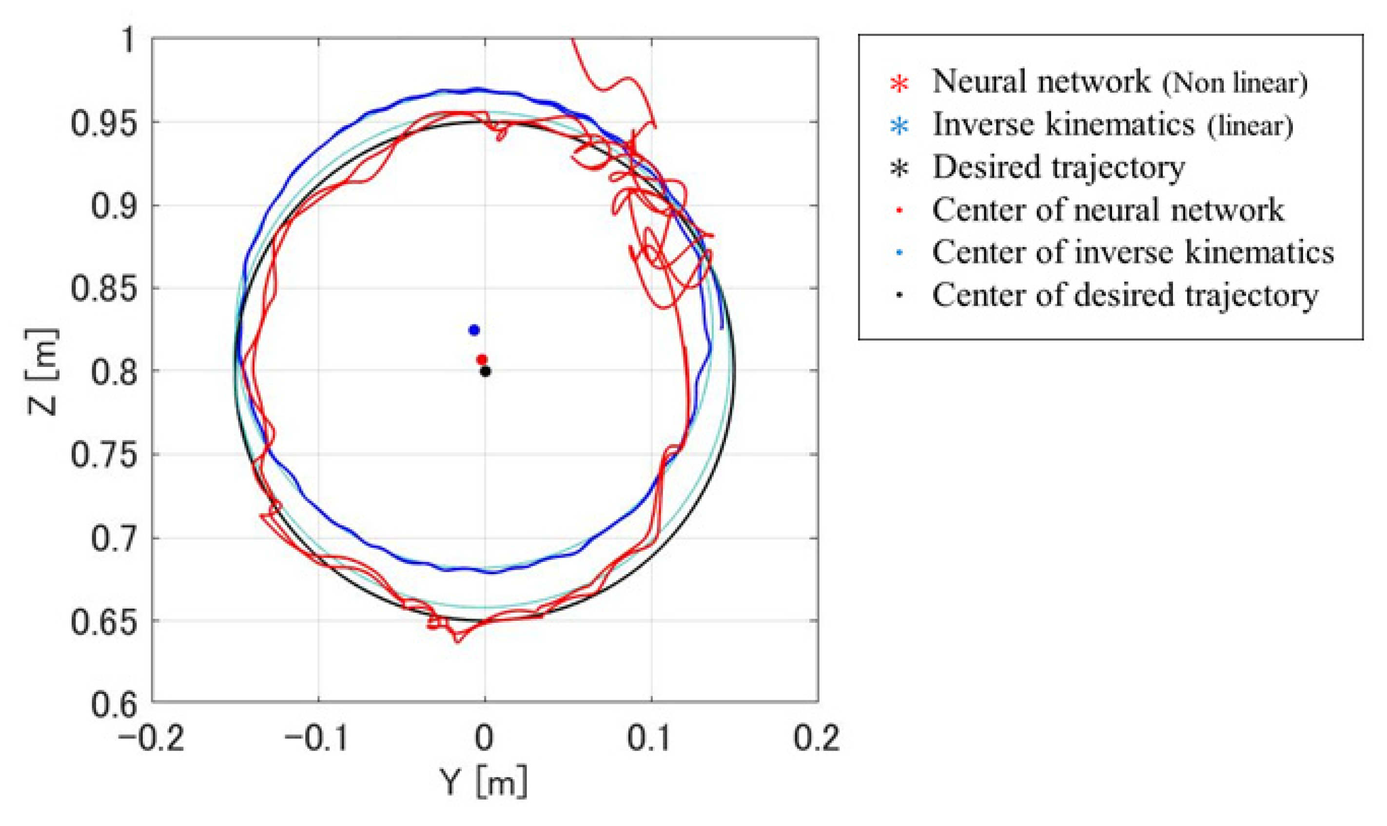
An implementation experiment was conducted using the inverse model trained with 0.29 s adjusted data. The control system configuration is shown in Figure 7, and the results are plotted in Figure 8.
Figure 7.
Results of experiment.
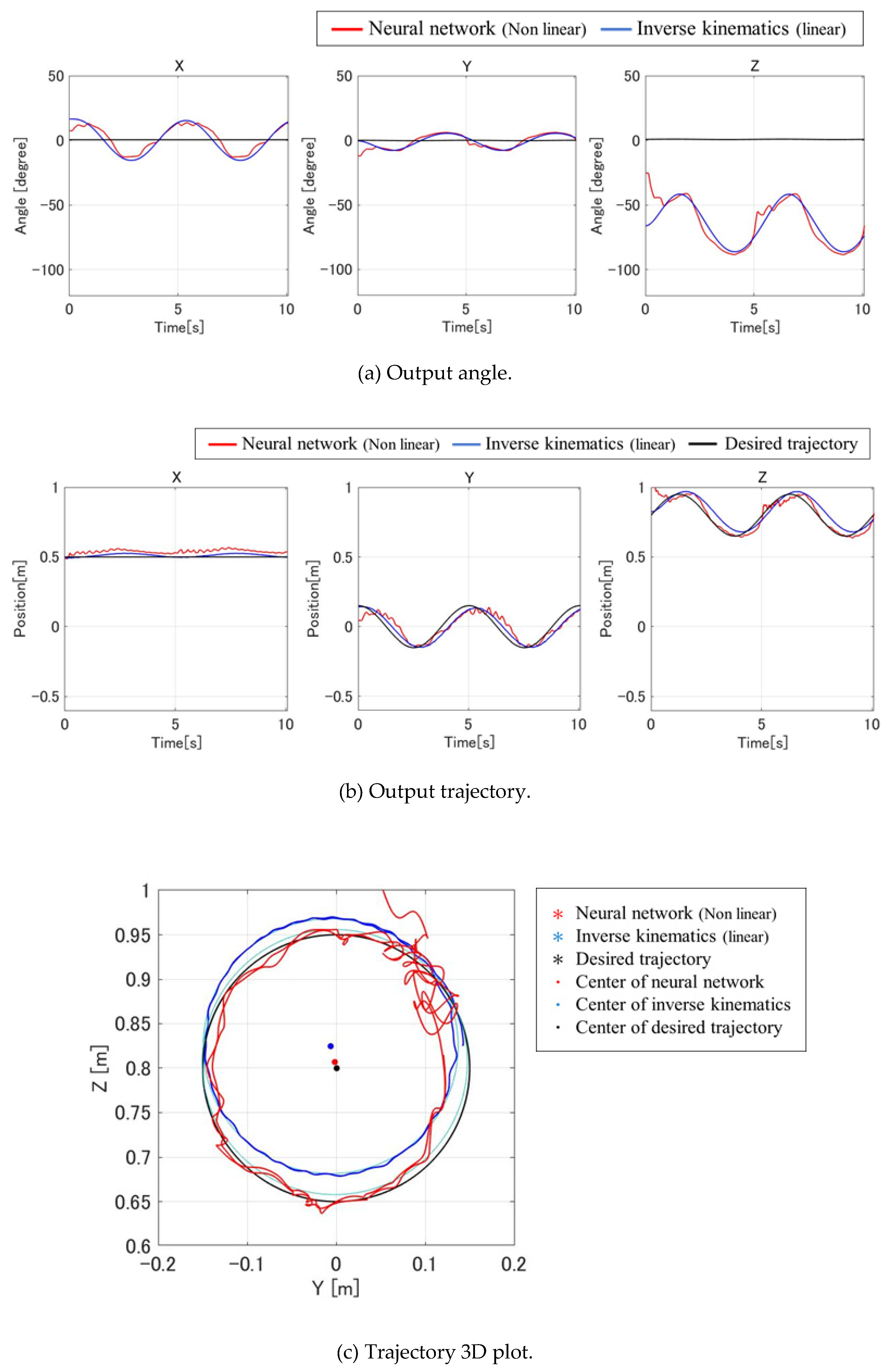

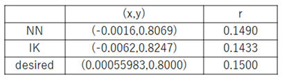
Table 3.
Approximated circle center and radius.
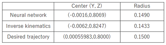
Although the generated trajectory was not smooth, the center and radius of the circular path were closer to the desired trajectory compared to results obtained using inverse kinematics alone.
The lack of smoothness in the trajectory is attributed to the use of ideal inverse kinematics angles for training, which do not reflect the actual motor dynamics. As the motor cannot instantly replicate sharp angle changes, the trained model output trajectories that the hardware could not feasibly follow. This suggests that improved performance may be achieved by incorporating both motor input and output angles into future training sets to better capture system behavior and constraints.
There was also a large deviation between the trajectory of the first and second revolutions. However, compared to the inverse kinematics output trajectory, the center point and radius of the circle approximated were closer to the target trajectory. The approximated circular path parameters are shown in Table 3.
While the inverse model enabled the manipulator to follow a roughly circular trajectory, the output trajectory was not smooth. In particular, a significant deviation was observed between the first and second revolutions. However, compared to the trajectory generated using inverse kinematics, the approximated circle’s center and radius were notably closer to the target values. This improvement suggests that the neural network successfully captured the dynamic characteristics of the actual hardware, partially compensating for structural and actuation inaccuracies.
To investigate the cause of the observed discontinuities, it is important to consider the training data used. In this study, only the inverse kinematics output angles were employed during training—these angles represent ideal trajectories calculated directly from the desired end-effector path. However, in practice, the motor cannot perfectly follow abrupt angle changes due to mechanical constraints and response time limitations. As a result, the inverse model, having learned from ideal angles, produced control signals that exceeded the real-time capabilities of the hardware.
This mismatch likely caused the physical system to fall out of synchronization with the model output, leading to unsmooth and inconsistent trajectory execution. To resolve this, it is recommended that future model training incorporates both the motor input and actual output angles, enabling the network to learn realistic dynamics and generate feasible control signals.
Further analysis is presented in Figure 8 and Table 4, which reaffirm that while the trajectory shape improved relative to traditional inverse kinematics control, smoothness and consistency still require enhancement through more representative training data.
Figure 8.
Results of experiment.
The results of this study demonstrate that neural networks—when trained with delay-compensated data—can effectively model the nonlinear and dynamic characteristics of flexible manipulators. The forward model accurately captured the relationship between joint angles and end-effector position, while the inverse model, although less stable, achieved improved tracking performance over classical inverse kinematics approaches when trained on temporally aligned datasets.
4. Discussion
Compared to the work of Kume et al. [1], who applied a hierarchical neural network to a 2-DOF flexible manipulator, our study extends the concept to a 3-DOF system operating in three-dimensional space. Kume’s model achieved satisfactory angle control in a planar setting but did not address spatial trajectory tracking or system delays. By incorporating delay compensation through a time lead in the training data, we addressed this limitation and demonstrated a notable improvement in trajectory accuracy. Our implementation experiment further showed that the neural network was able to internalize system-specific nonlinearities—such as elastic delay and mechanical asymmetry—which conventional model-based controllers do not inherently handle.
In comparison, Gao et al. [10] applied neural networks to a two-link flexible manipulator using the assumed mode method and achieved effective trajectory tracking. However, their approach relied on explicit modeling of the system’s dynamics and modal frequencies, whereas our study adopts a model-free learning paradigm. This shift reduces dependency on physical system identification but highlights the sensitivity of data-driven models to training data alignment, as evidenced by the performance deterioration in our uncorrected inverse model.
Sun et al. [12] proposed a fuzzy-neural hybrid system for a single-link flexible manipulator. While they reported improvements in trajectory accuracy and vibration suppression, their system was limited to low-DOF tasks and did not explicitly address joint-specific actuation delays. In contrast, our study showed that adjusting training data on a per-joint basis (e.g., using distinct propagation delay approximations) could enhance tracking fidelity, especially for high-DOF manipulators.
Moreover, our findings resonate with Chen and Wen [13], who used recurrent neural networks (RNNs) to model forward and inverse dynamics in robotic manipulators. They noted the difficulty in ensuring stability and continuity in inverse models—a challenge we also faced. While RNNs inherently handle temporal sequences, our approach demonstrated that even feedforward architectures can be effective when data is carefully prepared to align causal relationships.
Despite these advancements, the inverse model in our implementation experiment failed to produce a smooth circular trajectory. This is attributed to the training data using only inverse kinematics angles, which represent ideal, discontinuous signals that the hardware cannot follow. The resulting control signals exceeded the actuator’s capacity, causing trajectory distortions. This observation supports the conclusion of Abe [11], who emphasized the importance of incorporating actual motor behavior into learning systems for improved real-world applicability.
To resolve this, future work should consider a dual-input training strategy, where both the motor input and measured output angles are used. This would allow the neural network to learn the actuator’s dynamic limits and provide more realistic outputs. Additionally, per-joint delay compensation based on physical propagation speeds could be incorporated to further improve accuracy.
8. Conclusions
This study investigated the trajectory control of a 2-link, 3-DOF flexible manipulator using neural network-based forward and inverse models. Unlike conventional rigid-body control strategies, our approach leveraged data-driven modeling to account for system nonlinearities, elastic deformations, and actuation delays.
The forward model demonstrated strong correlation between joint angles and end-effector positions, accurately reflecting the spatial dynamics of the manipulator. The inverse model, though initially limited by phase mismatch in training data, showed significant improvement when delay-compensated trajectories were introduced—particularly with a 0.29-second time lead, which minimized mean squared error and improved trajectory tracking fidelity.
Simulation and implementation experiments validated the effectiveness of the neural network-based control scheme. In comparison to classical inverse kinematics, the proposed method achieved a trajectory closer to the desired circular path, with improved radius and center point estimation. However, the output trajectory remained unsmooth due to the use of idealized inverse kinematics angles in the training process, which failed to capture the actual motor dynamics.
To further enhance performance, future work should focus on incorporating both motor input and output angles into the training dataset, allowing the network to learn more realistic control strategies. Additionally, introducing joint-specific delay compensation and exploring recurrent or hybrid network architectures may help resolve discontinuities in inverse model outputs.
Overall, this study highlights the potential of neural networks as a powerful alternative to model-based control in flexible manipulators, particularly in systems where mechanical compliance and nonlinear dynamics hinder traditional approaches.
Author Contributions
Conceptualization, M.S. M.T. and W.N.; methodology, M.S. and W.N.; software, J.M and M.T; validation, M.S., M.T, J.M. and W.N.; formal analysis, M.T. and W.N.; investigation, M. T. and J.M.; resources, M.S. and M.T.; data curation, M.T.; writing—original draft preparation, M.S. and M.T.; writing—review and editing, J.M. and W.N.; visualization, M.T. and W.N.; supervision, M.S.; project administration, M.S.; funding acquisition, M.S. All authors have read and agreed to the published version of the manuscript.
Funding
This research supported by grants-in-aid for the promotion of regional industry-university-government collaboration from the Cabinet Office in Japan.
Data Availability Statement
All data underlying the results are available as part of the article and no additional source data are required.
Acknowledgments
This work was partially supported by grants-in-aid for regional industry-university-government collaboration from the Cabinet Office in Japan.
Conflicts of Interest
The authors declare no conflict of interest.
References
- Kume, S., Sasaki, M., Ito, S. Control of a Flexible Manipulator Using an Immune Controlled Adaptive Learning Neurocontroller. In Proceedings of the 18th MAGDA Conference of the Japan Society of AEM in Tokyo; 2009; pp. 291–296. [Google Scholar]
- Hideo Saito. Fundamentals of Industrial Vibration, (22nd edition; Yokendou Co., Ltd., 2006. [Google Scholar]
- Haruhisa Kawasaki. Fundamentals of Robotics, 2nd edition; Morikita Publishing Co., Ltd., 2019. [Google Scholar]
- Tetsuro Yabuta, Takayuki Yamada. Applied Physics 1991, 60, 577–580.
- M. Sasaki, H. Asai, M. Kawafuku and Y. Hori. Self-Tuning Control of a Translational Flexible Arm Using Neural Networks Proc. 2000 IEEE International Conference on Systems, Man, and Cybernetics, pp.3259-3264 (2000-10).
- Minoru Sasaki, Haruki Murasawa and Satoshi Ito. Control of a two-link flexible manipulator using neural networks. In Proceedings of SPIE, ICMIT 2007 Mechatronics, MEMS, and Smart Materials; 2007; Volume 6794, Part 1 of 2 Parts, p. 679421Y-1-679421Y-6. [Google Scholar]
- Minoru Sasaki, Akihiro Asai, Toshimi Shimizu, and Satoshi Ito. Self-Tuning Control of a Two-Link Flexible Manipulator using Neural Networks. Proceedings of ICCAS-SICE International Conference 2009 (CD-ROM), Fukuoka; 2009. Available online: https://ieeexplore.ieee.org/document/5335303.
- Waweru Njeri, Minoru Sasaki, Kojiro Matsushita. Gain tuning for high speed vibration control of a multilink flexible manipulator using artificial neural network. Transaction of ASME Journal of Vibration and Acoustics, 13 March 2019. [Google Scholar] [CrossRef]
- Minoru Sasaki, Nobuto Honda, Waweru Njeri, Kojiro Matsushita, Gain tuning using neural network for Contact force control of flexible arm. Journal of Sustainable Research in Engineering 2020, 5, 139–149.
- Gao, H. , He, W., Zhou, C., Sun, C. Neural Network Control of a Two-Link Flexible Robotic Manipulator Using Assumed Mode Method. IEEE Transactions on Industrial Informatics 2019, 15, 755–765. [Google Scholar] [CrossRef]
- Abe, A. Trajectory Planning for Flexible Cartesian Robot Manipulators Using Artificial Neural Networks. Robotica 2011, 29, 797–804. [Google Scholar] [CrossRef]
- Sun, C. , Gao, H., He, W., Yu, Y. Fuzzy Neural Network Control of a Flexible Robotic Manipulator. IEEE Transactions on Neural Networks and Learning Systems 2018, 29, 5214–5227. [Google Scholar] [CrossRef] [PubMed]
- Chen, S., Wen, J.T. Neural-Learning Trajectory Tracking Control of Flexible-Joint Robot Manipulators with Unknown Dynamics. 2020 IEEE International Conference on Robotics and Automation (ICRA); 2020. [Google Scholar] [CrossRef]
- Shaoqing Li, Lingcong Meng, Kai Fang and Fucai Liu. Neural Network Adaptive Inverse Control of Flexible Joint Space Manipulator Considering the Influence of Gravity. Sensors 2024, 24, 6942. [Google Scholar] [CrossRef] [PubMed]
- Xiaofei Chen, Han Zhao, Shengchao Zhen, Xiaoxiao Liu and Jinsi Zhang, Fixed-Time Adaptive Neural Network-Based Trajectory Tracking Control for Workspace Manipulators. Actuators 2024, 13, 252; [CrossRef]
Figure 1.
Setup of the flexible manipulator. a) Actual flexible manipulator (b) Illustration of the manipulator setup.
Figure 1.
Setup of the flexible manipulator. a) Actual flexible manipulator (b) Illustration of the manipulator setup.
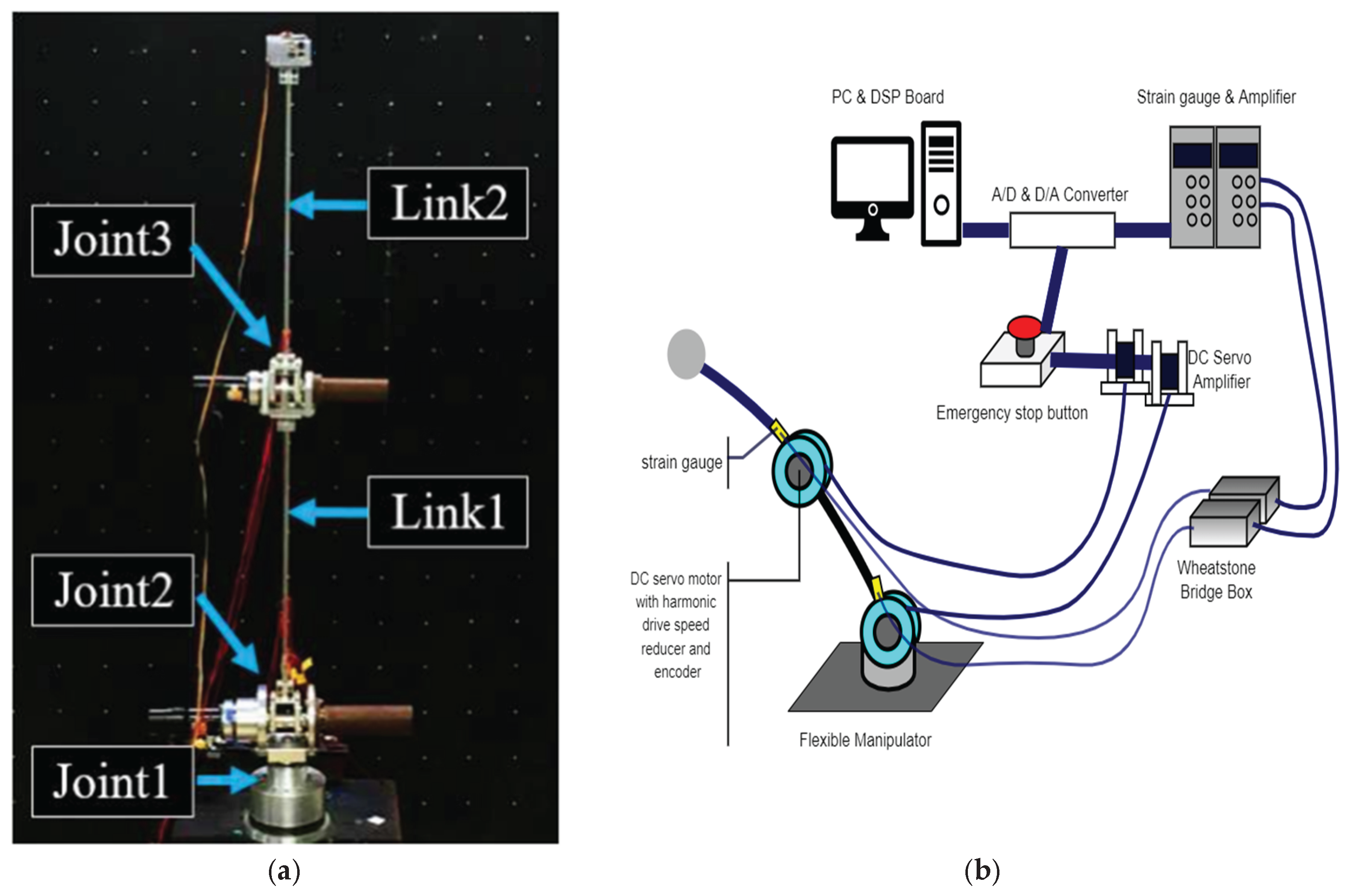
Figure 2.
Block diagram of experiment.
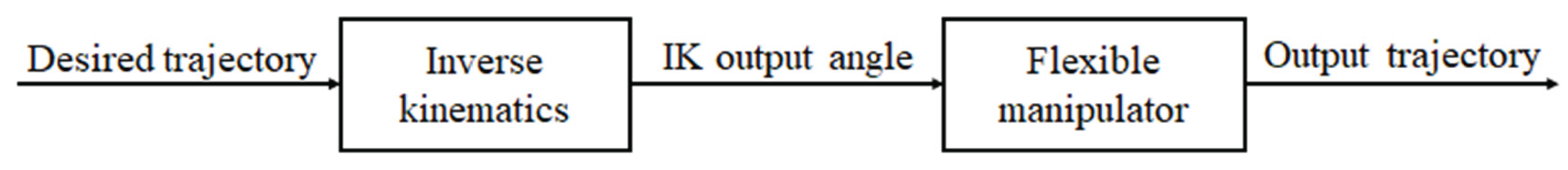
Figure 3.
Verification of control scheme.
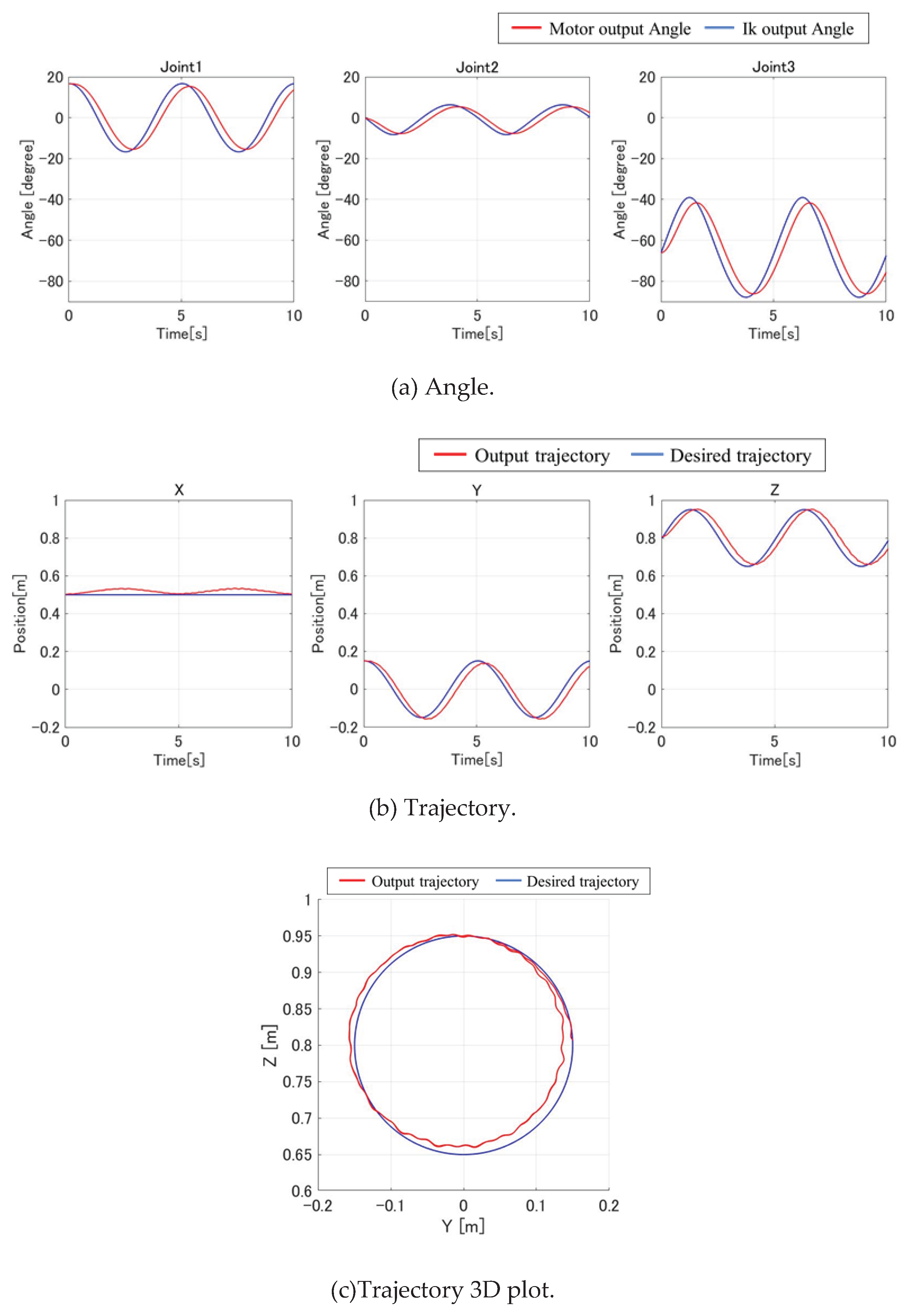
Figure 4.
Learning data of neural network.
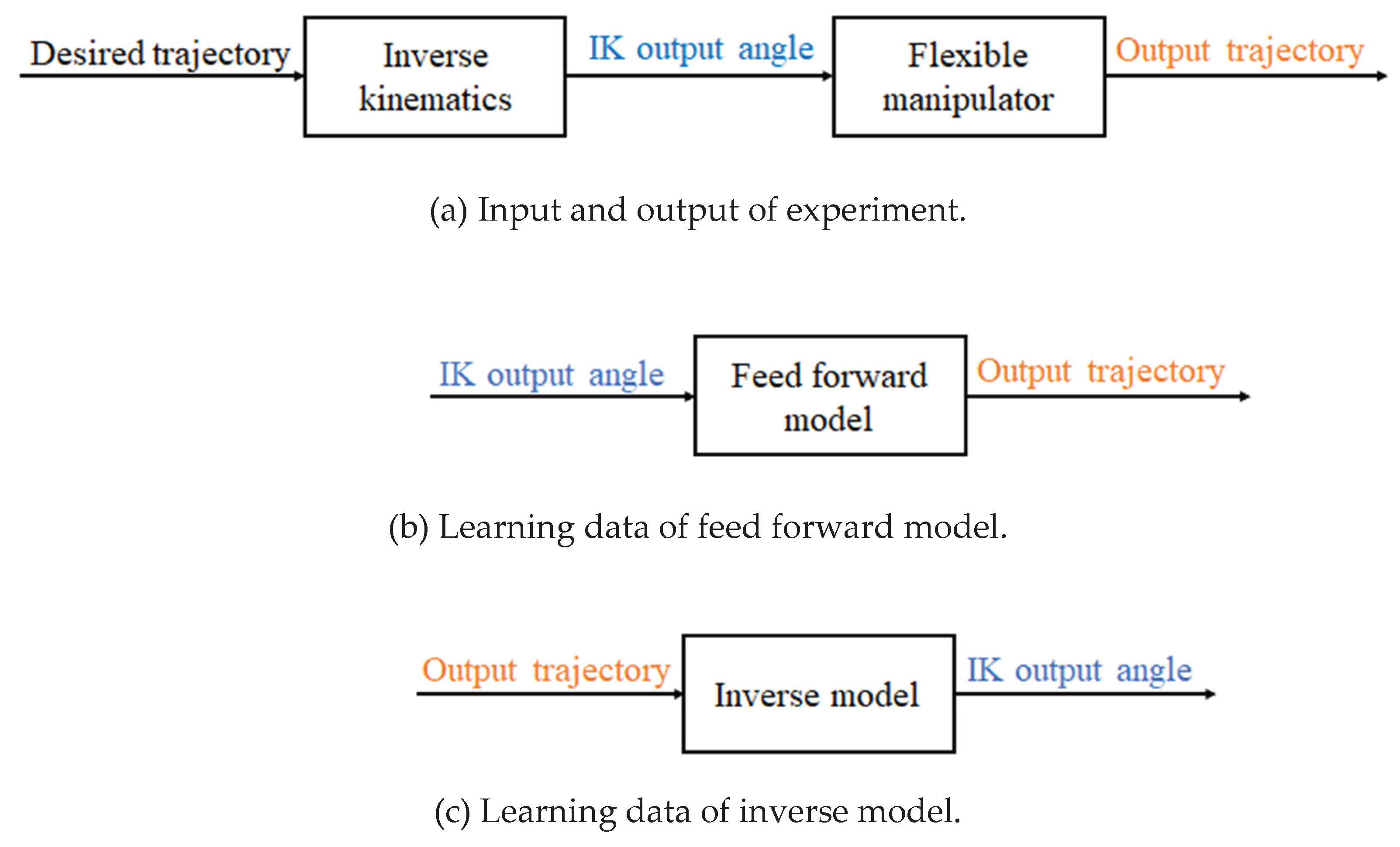
Figure 5.
Results of training neural network.
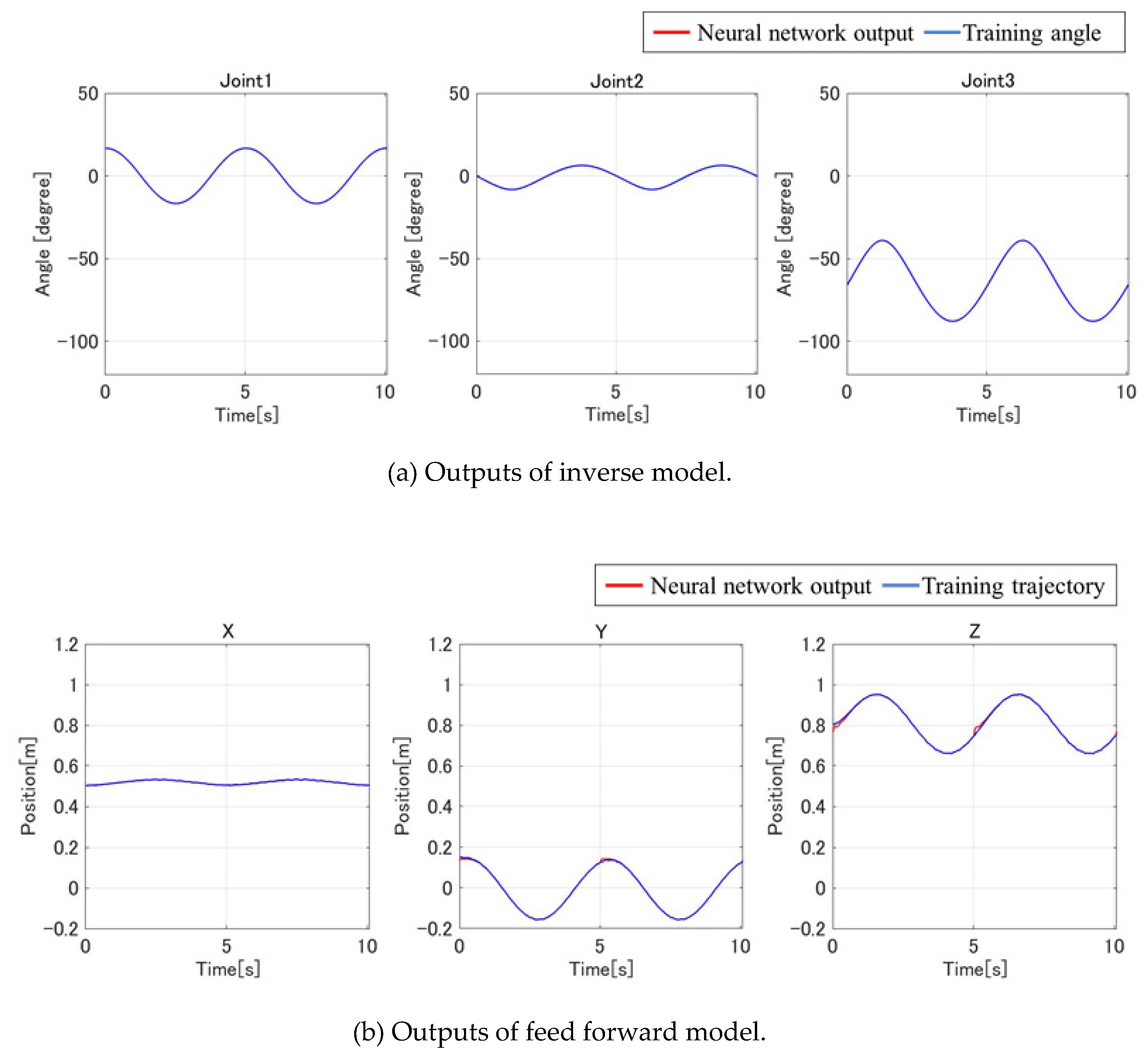
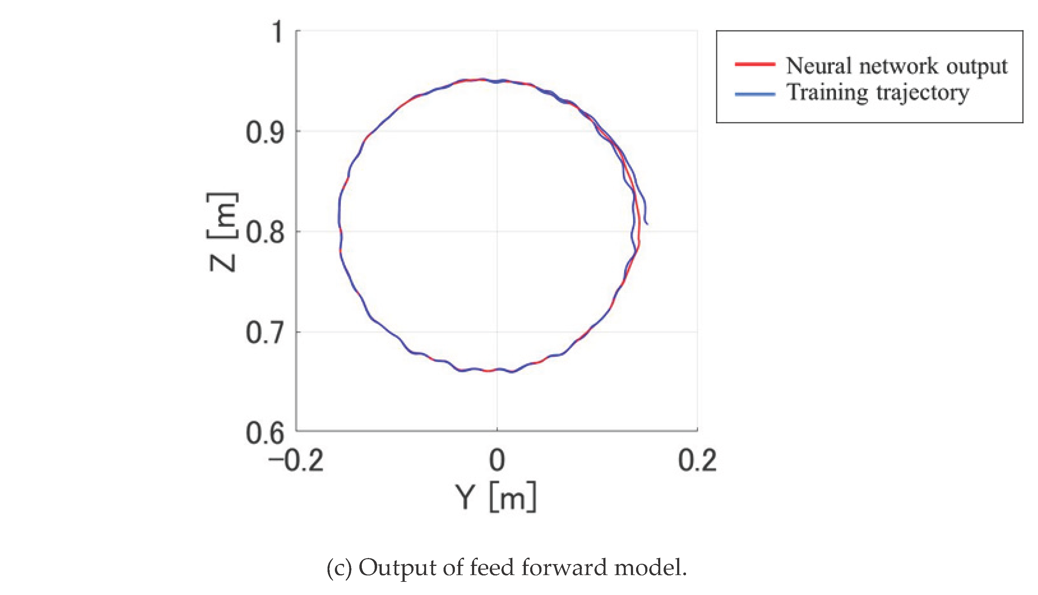
Figure 6.
Results of experiment.
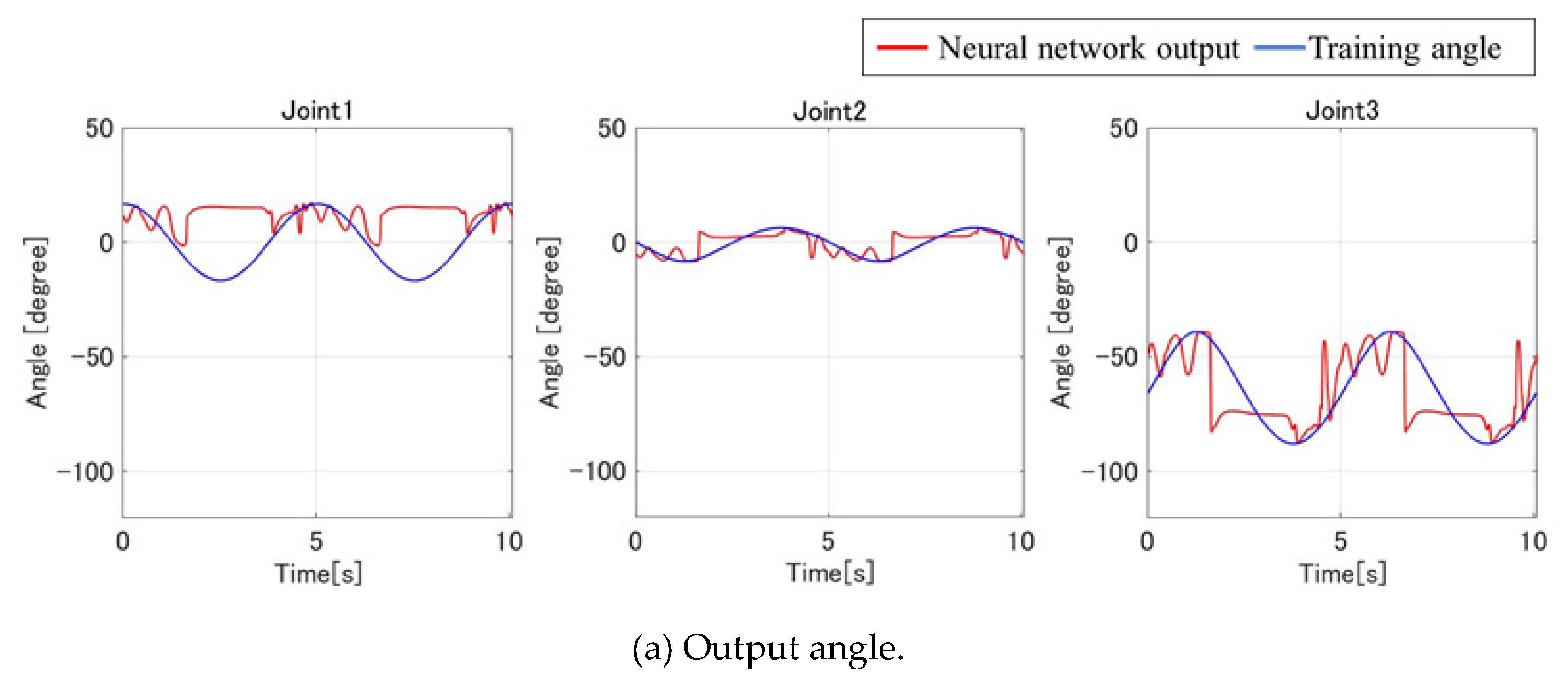
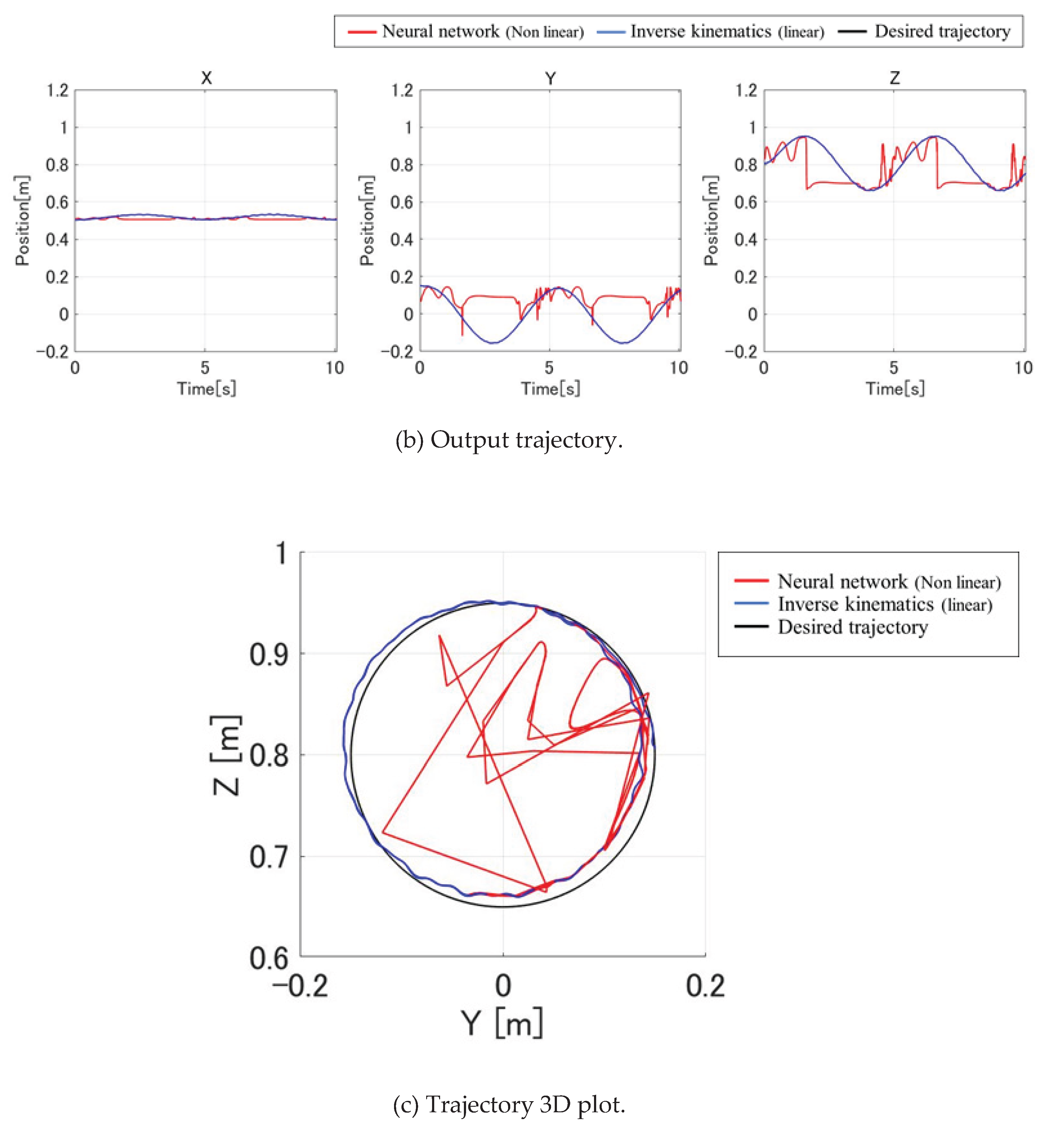
Figure 7.
Result of simulations.
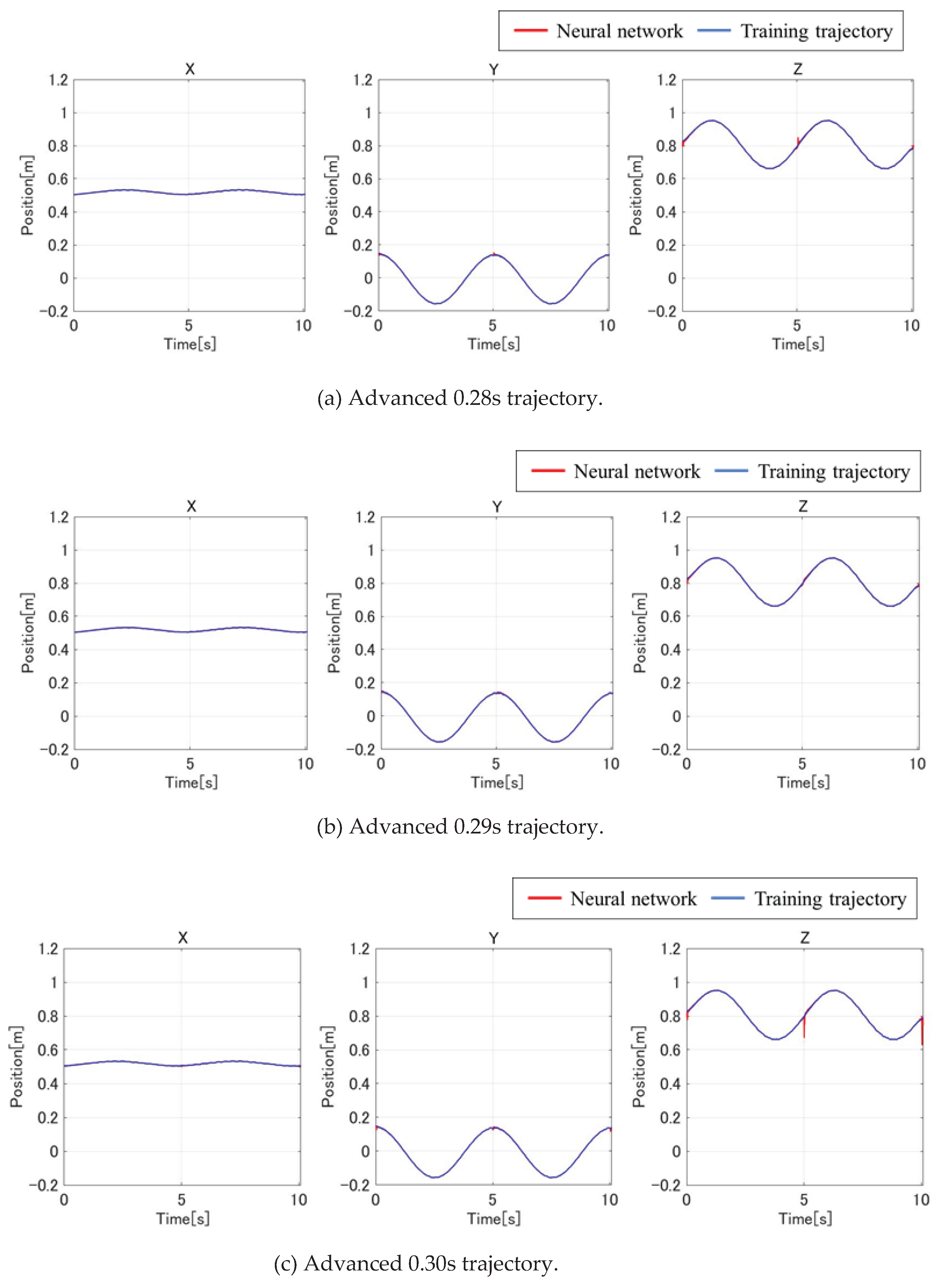
Table 1.
Mechanical and electrical specifications of the flexible manipulator.
| Component | Specification |
| Servo Motor 1 (Joint 1) | Type: V850-012EL8; Voltage: 80 V; Current: 7.6 A; Power: 500 W; Speed: 2500 rpm; Torque: 1.96 N·m; Inertia: 0.60×10⁻³ kg·m²; Mass: 4.0 kg |
| Servo Motor 2 (Joint 2) | Type: T511-012EL8; Voltage: 75 V; Current: 2 A; Power: 100 W; Speed: 3000 rpm; Torque: 0.34 N·m; Inertia: 0.037×10⁻³ kg·m²; Mass: 0.95 kg |
| Servo Motor 3 (Joint 3) | Type: V404-012EL8; Voltage: 72 V; Current: 1 A; Power: 40 W; Speed: 3000 rpm; Torque: 0.13 N·m; Inertia: 0.0084×10⁻³ kg·m²; Mass: 0.4 kg |
| Encoder | Resolution: 1000 P/R; Reduction Ratio: 1/100 |
| Harmonic Drive - Joint 1 | Type: CSF-40-100-2A-R-SP; Ratio: 1/100; Spring Constant: 23 N·m/rad; Inertia: 4.50×10⁻⁴ kg·m² |
| Harmonic Drive - Joint 2 | Type: CSF-17-100-2A-R-SP; Ratio: 1/100; Spring Constant: 1.6×10⁻⁴ N·m/rad; Inertia: 0.079×10⁻⁴ kg·m² |
| Harmonic Drive - Joint 3 | Type: CSF-14-100-2A-R-SP; Ratio: 1/100; Spring Constant: 0.71×10⁻⁴ N·m/rad; Inertia: 0.033×10⁻⁴ kg·m² |
| Link 1 | Material: Stainless Steel; Length: 0.44 m; Radius: 0.0005 m |
| Link 2 | Material: Aluminum; Length: 0.44 m; Radius: 0.004 m |
| Strain Gauge | Type: KGF-2-120-C1-23L1M2R |
Table 2.
Trigger of training end.
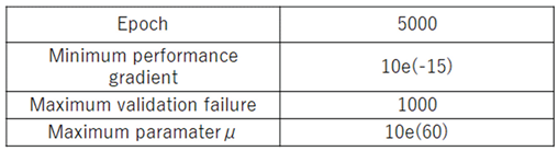
Table 3.
Mean squared errors.
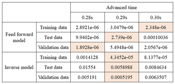
Table 4.
Centers and radiuses of circle.
Disclaimer/Publisher’s Note: The statements, opinions and data contained in all publications are solely those of the individual author(s) and contributor(s) and not of MDPI and/or the editor(s). MDPI and/or the editor(s) disclaim responsibility for any injury to people or property resulting from any ideas, methods, instructions or products referred to in the content. |
© 2025 by the authors. Licensee MDPI, Basel, Switzerland. This article is an open access article distributed under the terms and conditions of the Creative Commons Attribution (CC BY) license (http://creativecommons.org/licenses/by/4.0/).
Copyright: This open access article is published under a Creative Commons CC BY 4.0 license, which permit the free download, distribution, and reuse, provided that the author and preprint are cited in any reuse.


