
Submitted:
17 June 2025
Posted:
17 June 2025
You are already at the latest version
Abstract
Digital elevation model (DEM), as the fundamental units of terrain morphology, are crucial for understanding surface processes and land use planning. However, automated classification faces challenges due to inefficient terrain feature extraction from raw LiDAR point clouds and the limitations of traditional methods in capturing fine-scale topographic variations. To address this, we propose a novel hybrid RNN-CNN framework that integrates multi-scale TPI features to enhance both DEM generation. Our approach first models voxelated LiDAR point clouds as spatially ordered sequences, using recurrent neural networks (RNNs) to encode vertical elevation dependencies and convolutional neural networks (CNNs) to extract planar spatial features. By incorporating TPI as a semantic constraint, the model learns to distinguish terrain structures at multiple scales. Residual connections refine feature representations to preserve micro-topographic details during DEM reconstruction. Extensive experiments in the complex terrains of Jiuzhaigou demonstrate that our lightweight hybrid framework not only achieves excellent DEM reconstruction accuracy in both flat areas and complex terrains, but also improves computational efficiency by more than 24.9% on average compared to traditional interpolation methods, making it highly suitable for resource-constrained applications.
Keywords:
convolutional neural network (CNN)
; recurrent neural network (RNN)
; Topographic Position Index (TPI)
; light detection and ranging (LiDAR)
; digital elevation model (DEM)
1. Introduction
Digital Elevation Models (DEMs) play a crucial role in various geospatial applications that significantly impact the study of the ecological environment and natural resourcese [1,2]. Despite advancements in the use of high-resolution DEMs and Geographic Information Systems (GIS), automating the reconstruction of fine-scale DEM remains a complex and underexplored challenge. This issue is particularly important because accurate reconstruction of DEM is critical for various applications such as ecological modeling [3], risk analysis [4], and environmental management[5,6,7,8].Consequently, the development of automated algorithms capable of transforming raw point cloud data into high-precision DEMs is essential for improving the efficiency and accuracy of digital terrain modeling workflows. [9].
Current methodologies for DEM reconstruction can be comprehensively categorized into three distinct and well-established main types: traditional interpolation methods, machine learning approaches, and deep learning techniques, each representing different philosophical approaches to terrain modeling and data processing. Traditional computational approaches, which include fundamental techniques such as nearest neighbor interpolation [11] and linear interpolation methods, are characterized by their computational simplicity and operational efficiency. These conventional methods have been widely adopted due to their straightforward implementation and minimal computational overhead. However, despite their practical advantages, they frequently encounter significant difficulties when attempting to capture fine-scale terrain features and topographic details. Furthermore, these traditional methods demonstrate notable inadequacy when confronted with the complex task of handling heterogeneous landscapes that exhibit varying terrain characteristics and spatial complexity [12]. More sophisticated and technically advanced techniques have been developed to address some of these fundamental limitations. These enhanced approaches encompass a range of methodologies including morphological filtering techniques [13], slope-based filtering algorithms [14] that utilize specific threshold criteria for terrain classification, and comprehensive segmentation-based filtering algorithms [15] that partition the landscape into distinct topographic units. While these advanced techniques demonstrate measurably improved performance compared to their traditional counterparts, they continue to exhibit significant sensitivity to data noise and environmental interference. Additionally, these methods typically necessitate extensive manual preprocessing procedures and parameter tuning, which can be both time-consuming and require substantial domain expertise [16].In response to these persistent limitations and the growing demand for more robust solutions, machine learning-based methodologies have progressively emerged as promising alternatives in the field of DEM generation. These innovative approaches fundamentally reframe the DEM generation process as a sophisticated regression problem that can be solved through statistical learning techniques. Advanced algorithms including decision trees with hierarchical splitting criteria, support vector machines (SVM) with kernel-based transformations [17], and random forests (RF) [18,19] ensemble methods have been successfully implemented to tackle this challenge. These machine learning approaches strategically leverage a diverse array of geospatial features including point density distributions, local slope characteristics, and comprehensive neighborhood statistical measures to inform their predictive models [20,21,22,23,24]. While these machine learning methods demonstrate notable improvements in adaptability to complex and varied terrain conditions, their practical effectiveness continues to be heavily dependent on a fundamental assumption. This critical assumption requires that training datasets and testing datasets maintain similar spatial distributions and geomorphological characteristics. Consequently, this dependency significantly restricts their generalizability across different geographic regions and terrain types. The performance of these methods exhibits considerable variation when applied across different geomorphic regions with distinct topographic signatures. Moreover, maintaining large-scale spatial consistency remains a persistent challenge that compromises the overall reliability of these approaches [25,26,27].
With the unprecedented rapid advancement and maturation of deep learning technologies in recent years, entirely new possibilities and opportunities have emerged for substantially improving model generalization capabilities and enhancing spatial coherence in DEM reconstruction tasks [28,29,30,31]. Convolutional Neural Networks (CNNs) [32,33], which represent a paradigm shift in spatial data processing, possess the remarkable ability to effectively capture complex two-dimensional spatial patterns and hierarchical feature representations. This inherent capability enables these networks to achieve superior learning of intricate topographic features and terrain characteristics [34]. Through this enhanced learning capacity, CNNs successfully overcome many of the fundamental limitations that have historically plagued traditional machine learning approaches in geospatial applications [35]. Although several pioneering research studies have demonstrated successful applications of deep learning methodologies to high-resolution DEM reconstruction tasks [36,37,38,39], most of these studies focus on reconstructing high-accuracy DEMs from low-accuracy DEMs. In contrast, only a few studies have achieved the derivation of highly accurate DEMs from Digital Surface Models (DSMs) through sophisticated neural network architectures [40]. However, despite these encouraging developments and technological advances, the challenge of directly generating high-precision DEMs from raw LiDAR point clouds continues to represent a significant and largely unresolved technical challenge. This particular application requires handling the inherent complexity and irregular nature of point cloud data while maintaining the spatial accuracy and topographic fidelity necessary for high-quality DEM products.
To overcome these challenges, we propose an innovative hybrid RNN-CNN framework, which integrates multi-scale Topographic Position Index (TPI) features to achieve the coordinated optimization of high-precision DEM reconstruction. The TPI method is one of the most widely used techniques for landform classification. By calculating the difference in elevation between a given point and its surrounding area, TPI helps in identifying ridges, valleys, peaks, and other landforms. The approach proposed by Jennes [41] and Weiss [42] utilizes fixed neighborhood sizes to calculate the TPI and classify landforms. In order to obtain a more refined DEM, we introduced TPI. The method flow is divided into two core links: first, the voxelized LiDAR point cloud is modeled as a spatial ordered sequence, and the vertical elevation dependency is encoded by RNN, combined with CNN to extract planar spatial features, and the feature representation is optimized through the residual connection mechanism to complete the reconstruction of high-resolution DEM, effectively retaining the micro-undulation details of the terrain; on this basis, the multi-scale TPI is integrated into the classification module as a semantic constraint, and the terrain structure differences at different scales are learned through the hybrid network architecture. In summary, this study constructed a DEM reconstruction method that takes into account elevation dependency, planar spatial features and multi-scale terrain semantic constraints by integrating the hybrid framework of RNN and CNN and multi-scale TPI features. It not only retains high-resolution terrain details, but also improves reconstruction accuracy through multi-scale landform structure learning, providing an innovative solution for high-precision DEM reconstruction.
Our method consists of three key innovations:
- We propose a hybrid RNN-CNN framework that integrates CNN for planar feature extraction and RNN for vertical dependency modeling to capture multi-dimensional terrain features.
- Our method innovatively integrates multi-scale TPI features, achieving breakthrough improvements in high-precision DEM reconstruction.
- Extensive experiments conducted in the complex terrain of Jiuzhaigou demonstrate that our lightweight model achieves comparable DEM reconstruction accuracy while reducing computational complexity by 24.9% compared to traditional methods.
The structure of this paper is as follows: Section 2 introduces our data. Section 3 details the proposed method and its innovations; Section 4 presents the experimental setup and results, highlighting the advantages of our method over traditional approaches; and finally, Section 5 discusses the implications of our research findings and potential future directions.
2. Data Set
The study area (Figure 1) is located in the northern part of Jiuzhaigou County, Aba Tibetan and Qiang Autonomous Prefecture, in the southern Minshan Mountain Range of northwest Sichuan, China. Situated in the Jiuzhaigou National Nature Reserve, it is part of a transitional zone between the southeastern Tibetan Plateau and the Sichuan Basin. The region lies at the boundary of China’s first topographic step, where diverse geomorphological processes have occurred, including fluvial and glacial erosion, forming the predominant mountainous, hilly, and valley landscapes. The study area covers 65.9 , with elevation varying between 2306 m and 4306 m, and a relative elevation difference of 2000 m. Steep high mountains bound the eastern and western sides of the region, while a north-south trending high mountain canyon runs through the middle, creating five small alpine lakes in the northern part.

Table 1.
The details of the test data in Jiuzhaigou
| Properties of the Data | Contents |
|---|---|
| Attitude of points (m) | 1000 |
| Points density (pts/m2) | 15 |
| LiDAR scanner type | riegl-vg-1560i |
| Overlap of flight lines | 25% |
| Horizontal accuracy(cm) | 25-30 |
| Vertical accuracy | 15 |
| Flight platform | Cessna 208b aircraft |
3. Methodology
Our methodology is designed to transform raw LiDAR point clouds into high-fidelity DEMs through a lightweight design process.This process encompasses denoising, voxelization, feature extraction leveraging both RNNs and CNNs, and the application of topographic supervision via TPI constraints. By integrating the sequential processing strengths of RNNs with the spatial feature extraction capabilities of CNNs, and further enhancing the output with TPI-driven geomorphometric coherence, our approach yields terrain representations that excel in both accuracy and physiographic realism. This framework facilitates precise DEM reconstruction through elevation class predictions.
3.1. Voxelization and Spatially Ordered Sequences
In processing the raw LiDAR point cloud, we first perform preprocessing to eliminate noise and outliers, ensuring a high-quality dataset for subsequent analysis. Following this, the denoised points are systematically mapped onto a regular voxel grid defined by a uniform spatial resolution. Each voxel is uniquely identified by its coordinates within this grid, and for every horizontal position, we aggregate the elevation values of occupied voxels along the vertical dimension. These elevation values are meticulously ordered to construct a sequence that encapsulates the vertical profile at each location. This spatially ordered sequence representation is particularly advantageous in managing regions with heterogeneous point densities, as it selectively retains valid elevation data, thereby preserving the intricate three-dimensional geometry of the terrain in an efficient and organized manner. Mathematically, the spatial resolution of the voxel grid is defined as ( x, y, z), with each voxel centered at:
where are the minimum coordinates of the point cloud and are integer indices. At each horizontal location , we collect all occupied values and sort them in ascending order to form a variable-length sequence
where m is the number of nonempty voxels in that column. This “spatially ordered sequence” representation addresses the issue of empty voxels by only storing valid elevations and retains key geometric structure in a compact form.
Figure 2.
Illustration of the comprehensive workflow for generating a high-precision DEM from LiDAR point clouds. The process commences with denoising and voxelization of the raw input data, followed by ranking and embedding elevation values to capture vertical relationships. A RNN encodes the vertical context, while a CNN extracts spatial features, with the resulting representations fused via residual connections. The fused features are then decoded into a DEM under TPI constraints, and the output is refined through a threshold-based median filtering post-processing step to enhance topographic fidelity.
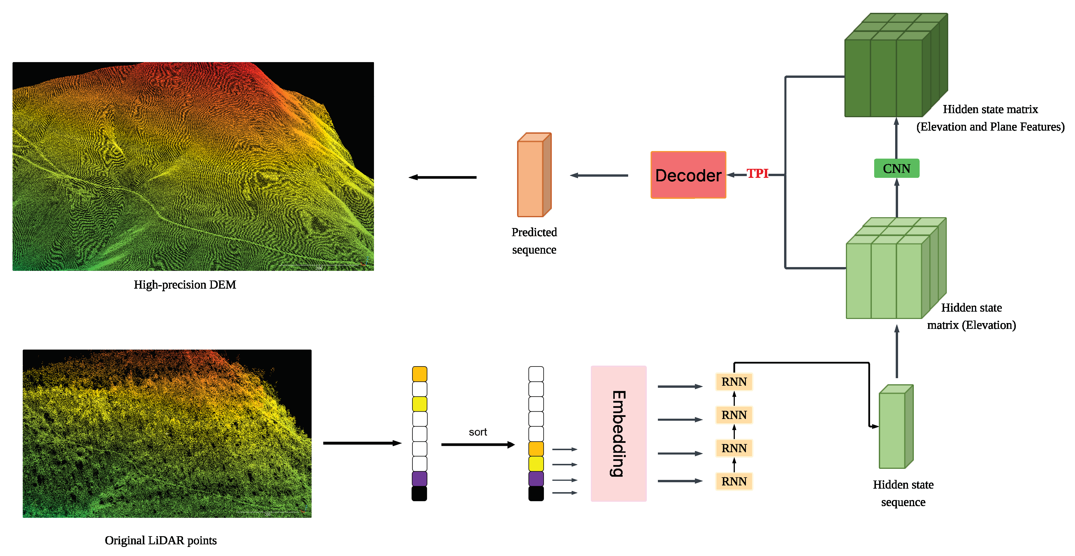
3.2. Elevation Index Representation and Encoding
To address the inherent variability and noise in raw elevation measurements, we employ a rank-based transformation strategy. Specifically, each elevation within a sequence is converted into its positional rank relative to other elevations at the same horizontal location. This ordinal representation emphasizes the vertical relationships among points, mitigating the influence of absolute elevation fluctuations and noise. Subsequently, these ranks are projected into a high-dimensional vector space through a learnable embedding mechanism, which encodes the structural dependencies and relational attributes of the elevation sequence. These embedded vectors serve as the foundational input for the sequence encoding phase, enabling robust modeling of vertical patterns across the terrain. For each elevation in , its rank is defined as:
and its embedding is:
where is a learnable embedding function (inspired by NLP embedding techniques) that produces d-dimensional vectors capturing semantic relationships among elevation ranks. These embeddings serve as the input to our sequence encoder.
3.3. Three-Dimensional Feature Extraction Framework
Given the computational demands of directly applying three-dimensional convolutions across the entire voxel grid, we adopt a hybrid processing paradigm that judiciously separates the extraction of vertical and horizontal features. This dual-strategy approach optimizes computational efficiency while ensuring that critical three-dimensional spatial information is retained, thereby supporting the generation of accurate and detailed DEMs.
3.3.1. Sequential Feature Modeling with RNNs
At each horizontal grid position, the sequence of embedded elevation ranks is processed by a Gated Recurrent Unit (GRU)-based recurrent neural network. The GRU architecture is particularly well-suited for this task, as it effectively captures long-range dependencies and local geometric nuances within the elevation sequence. By iteratively processing the sequence, the GRU distills a comprehensive representation of the vertical structure into its final hidden state. This compact encoding retains essential elevation details without requiring aggressive downsampling, thereby preserving the fidelity of the terrain’s vertical characteristics. For each position , the hidden state () is obtained through the GRU’s processing of the sequence ().
3.3.2. Spatial Feature Enhancement with CNNs
To integrate lateral spatial relationships into the feature set, the hidden states generated by the GRU are organized into a two-dimensional feature map aligned with the horizontal grid layout. This map is subsequently processed by a convolutional neural network employing a U-Net-inspired architecture. The CNN applies a series of downsampling and upsampling operations, augmented by residual connections, to extract multi-scale spatial features. These residual connections play a pivotal role in preserving fine-scale details from the RNN outputs across the convolutional layers, ensuring that the resulting feature set captures both broad spatial patterns and localized terrain variations. The CNN output is then fused with the original RNN hidden states through an additional residual linkage, creating a rich feature representation that balances vertical and horizontal terrain information. Mathematically, the fused feature is:
where is the feature extracted by the CNN.
3.4. Decoder Design and Operational Mechanism
The decoder constitutes a pivotal element of our methodology, tasked with synthesizing the final elevation predictions from the integrated features produced by the preceding stages. It leverages the complementary strengths of sequential and spatial processing to generate DEMs that accurately reflect the terrain’s multifaceted characteristics. The decoder employs a GRU-based recurrent neural network, complemented by an embedding layer for input processing and a fully connected layer for output mapping. This configuration enables the generation of elevation class predictions tailored to the quantized elevation space. The decoding process begins with a placeholder input, which is embedded into a high-dimensional space to establish the starting point for sequence generation. Subsequently, this embedded input is combined with the fused features from the encoder and CNN, providing a holistic context for elevation prediction. The GRU processes this integrated input in a single pass, producing an output that encapsulates the synthesized terrain information. This output is then transformed through a fully connected layer into logits representing quantized elevation classes, which are subsequently mapped to continuous elevation values. The residual connection ensures that intricate vertical details from the encoder are effectively incorporated into the decoding process, enhancing the reconstruction of complex terrain features. The predicted elevation () is obtained from the class prediction , where () is the probability of class k.
3.5. Incorporation of TPI Constraints
To ensure that the generated DEMs exhibit realistic topographic characteristics, we introduce supervision based on the Topographic Position Index (TPI) during the training phase. TPI serves as a localized metric that quantifies terrain features by comparing a point’s elevation to the average elevation of its surrounding neighborhood. At a given scale (s), TPI is computed as:
where is the set of neighbors within distance (s). We calculate TPI values for both predicted and ground-truth elevations across multiple scales. The TPI loss is defined as the mean squared difference between these values, aggregated over all grid cells and scales:
This loss is combined with the primary elevation classification objective, guiding the model to align predicted elevations with realistic topographic patterns. By enforcing TPI constraints at various scales, the model captures a spectrum of terrain features, from fine-scale details to broader landforms. The weighted TPI loss ensures a balance between elevation accuracy and geomorphometric fidelity, reducing artifacts and enhancing the realism of the DEM.
3.6. Post-Processing Refinement
To polish the predicted DEM and address residual noise, we implement a post-processing phase utilizing a threshold-based median filtering technique. For each grid cell, the median elevation of its immediate neighbors is computed. If the predicted elevation deviates from this median beyond a specified threshold, it is adjusted to the median value. This step mitigates isolated anomalies, such as spikes or depressions, while preserving genuine micro-topographic features by avoiding excessive smoothing. Mathematically, if , where is the neighborhood median, then is set to . This refinement ensures that the final DEM is both smooth and detailed, rendering it suitable for advanced terrain analysis and visualization applications.
4. DEM Reconstruction Results and Discussion
4.1. Visual Comparison Analysis
Figure 3 provides a comprehensive comparative analysis of DEMs that have been produced using various methodological approaches. This visual comparison effectively demonstrates the distinct differences in reconstruction quality and spatial accuracy across different interpolation techniques.From a detailed visualization and qualitative assessment standpoint, the comparative results reveal significant deficiencies in traditional interpolation approaches. Even when enhanced with the application of basic morphological filtering techniques designed to reduce noise artifacts, both the linear interpolation method and the nearest-neighbor interpolation method continue to yield DEMs that exhibit severe degradation in quality. These reconstructed terrain models are substantially and adversely affected by the presence of point cloud noise and the inclusion of misclassified points within the dataset. The cumulative impact of these data quality issues manifests in the generation of terrain surfaces that are characterized by excessive roughness and spatial discontinuity, rendering them unsuitable for high-precision applications.
Furthermore, these traditional interpolation methodologies demonstrate particularly pronounced performance deficiencies when applied to challenging topographic conditions. In areas characterized by steep slope gradients and complex terrain morphology, these conventional methods exhibit especially poor reconstruction capabilities. The limitations become most apparent in regions where the preservation of crucial terrain features is of paramount importance. Critical topographic elements such as mountain peaks, prominent ridgelines, and sharp terrain boundaries tend to undergo excessive smoothing processes during reconstruction. In the most severe cases, these distinctive terrain features may be completely lost or significantly diminished in the final DEM output. This systematic loss and degradation of important topographic characteristics fundamentally undermines the overall accuracy and reliability of the reconstructed DEM products. The implications of these reconstruction failures extend beyond simple visual artifacts, as they compromise the fundamental utility of the DEM for subsequent geospatial analyses and applications. For comprehensive and detailed visualizations that specifically illustrate the error characteristics and spatial distribution of inaccuracies inherent in traditional interpolation approaches, readers are directed to consult the supplementary analysis presented in Figure 4.
Our method successfully recovers terrain features while avoiding the over-smoothing artifacts prevalent in conventional approaches, demonstrating superior performance in complex terrains including detailed hilly regions and forest-covered mountainous areas. For a detailed visualization of the DEM generated by our method, see Figure 5. Through accurate capture of steep topographic gradients and preservation of critical geomorphological features (e.g., ridgelines, valley floors), the proposed framework outperforms traditional methods—an achievement enabled by our hybrid network architecture. This architecture synergistically combines CNNs for local spatial feature extraction with RNNs processing elevation-directional global information, while incorporating TPI supervision to mitigate erroneous elevation values, thereby fully exploiting the inherent spatial-structural relationships within point clouds to achieve enhanced DEM prediction accuracy.
4.2. Quantitative Accuracy Evaluation
In the evaluation of DEM quality, aside from qualitative visual analysis, accuracy is a critical metric. To comprehensively quantify the deviation between the predicted DEM and the actual terrain, we adopted the following evaluation metrics: root mean square error (RMSE) and mean absolute error (MAE). Their mathematical formulations are expressed as follows:
- RMSE:where, is the predicted elevation and is the corresponding reference value.
- MAE:providing a measure of the average absolute error across the DEM.
Table 2 presents a comprehensive and detailed quantitative accuracy assessment that systematically evaluates the performance characteristics of different interpolation methodologies. This tabular summary encompasses results from two distinct experimental scenarios, each designed to rigorously compare the effectiveness of our proposed method against well-established traditional interpolation approaches, specifically linear interpolation and nearest-neighbor interpolation techniques.
In Experiment 1, our newly developed model demonstrates exceptional performance capabilities with remarkably low error metrics. The proposed approach achieves a RMSE of 1.30 meters, indicating high precision in elevation predictions. Correspondingly, the MAE metric registers at 0.77 meters, further confirming the superior accuracy of our methodology. In stark contrast to these impressive results, the traditional linear interpolation method exhibits significantly degraded performance characteristics. This conventional approach yields a substantially elevated RMSE of 121.81 meters, representing nearly two orders of magnitude higher error than our proposed method. The corresponding MAE for linear interpolation reaches 103.29 meters, demonstrating consistent poor performance across both error metrics. Similarly, the nearest-neighbor interpolation technique produces comparably unsatisfactory results with an RMSE of 121.37 meters and an MAE of 102.69 meters, indicating that both traditional methods suffer from fundamental limitations in accuracy.
The Experiment 2, provides additional validation of our method’s superior performance and reinforces the consistent advantages over traditional approaches. In this experimental configuration, our innovative approach records an even more impressive RMSE of 1.06 meters, representing a slight improvement over the already excellent results from the first experiment. The MAE metric correspondingly shows enhanced performance with a value of 0.71 meters, demonstrating the robustness and reliability of our proposed methodology across different experimental conditions. Meanwhile, the traditional interpolation methods continue to exhibit substantially larger error magnitudes that underscore their inherent limitations. The linear interpolation method produces an RMSE of 110.48 meters and an MAE of 90.50 meters in this second experimental scenario. Concurrently, the nearest-neighbor interpolation approach yields an RMSE of 109.06 meters and an MAE of 88.80 meters, respectively. These consistently high error values across both experimental trials clearly demonstrate that traditional interpolation techniques are fundamentally inadequate for achieving the level of precision required for high-quality DEM reconstruction applications.
These results demonstrate that our method outperforms traditional interpolation by more than two orders of magnitude in both RMSE and MAE. The primary reason for this substantial gap is that our pipeline directly generates the DEM from raw point clouds: it automatically learns to filter non-ground points, correctly identifies ground returns, and, under TPI supervision, reconstructs a high-precision DEM. In contrast, the linear and nearest-neighbor approaches rely only on a simple morphological filter before interpolation, which fails to robustly remove non-ground points. By integrating end-to-end feature learning, our method both suppresses non-ground noise and preserves critical terrain details—hence the dramatic improvement in accuracy.
4.3. Computational Efficiency Analysis
Table 3 provides a detailed computational performance comparison that systematically evaluates the runtime efficiency characteristics of our proposed lightweight framework in direct comparison with established traditional interpolation techniques. This comprehensive analysis examines the execution time requirements across two distinct test datasets, demonstrating how our streamlined architecture achieves superior computational efficiency compared to both nearest-neighbor interpolation and linear interpolation methodologies.
In Experiment 1, our innovative approach demonstrates remarkable computational efficiency by completing the entire DEM generation process in a total execution time of 7.62 seconds. This impressive performance represents a substantial improvement over traditional methods, achieving approximately 35.5% faster processing speed compared to the nearest-neighbor interpolation technique, which requires 11.82 seconds for completion. Furthermore, our method exhibits even more pronounced advantages when compared to linear interpolation, demonstrating approximately 45.7% faster execution than the linear interpolation approach, which necessitates 14.05 seconds to complete the same DEM generation task.
The Experiment 2, provides additional validation of our method’s superior computational performance and confirms the consistency of these efficiency gains across different datasets. In this experimental trial, our proposed method achieves an even more impressive execution time of 6.86 seconds for complete DEM generation. This enhanced performance translates to approximately 24.9% faster processing compared to the nearest-neighbor interpolation method, which requires 9.14 seconds for completion in this experimental scenario. Similarly, our approach maintains significant computational advantages over linear interpolation, demonstrating approximately 40.2% faster execution than the linear interpolation technique, which necessitates 11.47 seconds to complete the equivalent processing task.
These comprehensive experimental results provide compelling evidence that our end-to-end computational framework consistently and significantly reduces processing time requirements across different datasets and experimental conditions. The performance improvements range from roughly one-quarter to nearly one-half reduction in processing time when compared to traditional interpolation techniques, demonstrating substantial and consistent computational advantages. The underlying mechanism responsible for these remarkable efficiency gains lies in our strategic architectural design approach. By systematically replacing computationally expensive neighborhood search operations and complex planar fitting procedures with a streamlined and lightweight RNN → 2D CNN processing pipeline, we have achieved a dual benefit of enhanced performance characteristics.
This innovative architectural approach not only delivers markedly higher accuracy in DEM reconstruction results but also simultaneously achieves significantly accelerated DEM generation processing speeds. The synergistic combination of improved accuracy and enhanced computational efficiency represents a substantial advancement over existing methodologies. Consequently, our proposed method demonstrates exceptional suitability for deployment in large-scale geospatial applications where extensive dataset processing is required. Additionally, the method proves highly advantageous for time-sensitive operational scenarios where rapid processing turnaround is essential. These characteristics make our approach particularly valuable for applications where both computational speed and reconstruction precision are critical requirements that must be simultaneously satisfied.
5. Conclusion
In this study, we proposed a lightweight method for reconstructing DEMs from LiDAR point clouds which effectively balances computational efficiency and feature representation. Experimental results on Jiuzhaigou datasets demonstrate that our streamlined approach not only outperforms traditional methods in RMSE and MAE metrics, but also achieves superior computational efficiency with 24.9% improvement in processing speed while excelling in complex, steep terrain by accurately capturing details such as ridges and valleys. Nevertheless, the method can still exhibit local detail distortion in extremely noisy or complex areas. However, our method is not without limitations. In some extremely complex or highly noisy regions, the model may still exhibit local detail distortions or gradient discontinuities. Future work will focus on several improvements: in data preprocessing, we plan to further refine noise suppression and outlier removal strategies to enhance reconstruction stability in complex regions; in model architecture, we will explore multi-scale fusion mechanisms to enhance feature representation across different spatial scales; and we will continue to optimize our lightweight network design and develop more efficient parallel computing schemes to further reduce computational complexity and improve large-scale data processing efficiency. Overall, this study provides an efficient, robust, and computationally lightweight solution for reconstructing DEMs from point clouds, offering significant advantages in resource-constrained environments while maintaining high precision. The proposed framework outlines clear directions for future improvements in accuracy, scalability, and computational efficiency.
Funding
This research was funded by National Key Research and Development Program of China [Grant No. 2024YFC3810802], [National Key R & D] grant number [2018YFB0504500], [National Natural Science Foundation of China] grant number [41101417] and [National High Resolution Earth Observations Foundation] grant number [11-H37B02-9001-19/22].
Conflicts of Interest
The authors declare no conflicts of interest.
References
- MacMillan, R. , Jones, R. K., & McNabb, D. H. (2004). Defining a hierarchy of spatial entities for environmental analysis and modeling using digital elevation models (DEMs). Computers, Environment and Urban Systems, 28(3), 175–200.
- Yang, J. , Xu, J., Lv, Y., Zhou, C., Zhu, Y., & Cheng, W. (2023). Deep learning-based automated terrain classification using high-resolution DEM data. International Journal of Applied Earth Observation and Geoinformation, 118, 103249.
- Siervo, V. , Pescatore, E., & Giano, S. I. (2023). Geomorphic analysis and semi-automated landforms extraction in different natural landscapes. Environmental Earth Sciences, 82(5), 128.
- Gallant, J. C. , & Austin, J. M. (2015). Derivation of terrain covariates for digital soil mapping in Australia. Soil Research, 53(8), 895–906.
- Armstrong, R. N. , &; Martz, L. W. (2003). Topographic parameterization in continental hydrology: A study in scale. Hydrological Processes, 17(18), 3763–3781. [Google Scholar]
- Wood, Sam W., Brett P. Murphy, and David MJS Bowman. "Firescape ecology: how topography determines the contrasting distribution of fire and rain forest in the south-west of the Tasmanian Wilderness World Heritage Area." Journal of Biogeography 38.9 (2011): 1807-1820.
- Bilodeau, M. F. , Esau, T. J., Zaman, Q. U., Heung, B., & Farooque, A. A. (2024). Enhancing surface drainage mapping in eastern Canada with deep learning applied to LiDAR-derived elevation data. Scientific Reports, 14(1), 10016.
- Li, B. , Lu, H., Wang, H., Qi, J., Yang, G., Pang, Y., Dong, H., &; Lian, Y. (2022). Terrain-Net: A highly-efficient, parameter-free, and easy-to-use deep neural network for ground filtering of UAV LiDAR data in forested environments. Remote Sensing, 14(22), 5798. [Google Scholar]
- Li, W. , & Hsu, C.-Y. (2020). Automated terrain feature identification from remote sensing imagery: A deep learning approach. International Journal of Geographical Information Science, 34(4), 637–660.
- Arun, Pattathal Vijayakumar. "A comparative analysis of different DEM interpolation methods." The Egyptian journal of remote sensing and space science 16.2 (2013): 133-139.
- Altman, Naomi S. "An introduction to kernel and nearest-neighbor nonparametric regression." The American Statistician 46.3 (1992): 175-185.
- Heritage, George L., et al. "Influence of survey strategy and interpolation model on DEM quality." Geomorphology 112.3-4 (2009): 334-344.
- Li, Yong, et al. "Airborne LiDAR data filtering based on geodesic transformations of mathematical morphology." Remote Sensing 9.11 (2017): 1104.
- Vosselman, George. "Slope based filtering of laser altimetry data." International archives of photogrammetry and remote sensing 33.B3/2; PART 3 (2000): 935-942.
- Lin, Xiangguo, and Jixian Zhang. "Segmentation-based filtering of airborne LiDAR point clouds by progressive densification of terrain segments." Remote Sensing 6.2 (2014): 1294-1326.
- Zhang, Keqi, et al. "A progressive morphological filter for removing nonground measurements from airborne LIDAR data." IEEE transactions on geoscience and remote sensing 41.4 (2003): 872-882.
- Mo, You, et al. "Integrated airborne LiDAR data and imagery for suburban land cover classification using machine learning methods." Sensors 19.9 (2019): 1996.
- Veronesi, F. , & Hurni, L. (2014). Random Forest with semantic tie points for classifying landforms and creating rigorous shaded relief representations. Geomorphology. 224, 152–160.
- Tan, Y.-C.; Duarte, L.; Teodoro, A.C. Comparative Study of Random Forest and Support Vector Machine for Land Cover Classification and Post-Wildfire Change Detection. Land 2024, 13, 1878. [Google Scholar] [CrossRef]
- Qian, Y.; Zhou, W.; Yan, J.; Li, W.; Han, L. Comparing Machine Learning Classifiers for Object-Based Land Cover Classification Using Very High Resolution Imagery. Remote Sens. 2015, 7, 153–168. [Google Scholar] [CrossRef]
- Hengl, T. , & Rossiter, D. G. (2003). Supervised Landform Classification to Enhance and Replace Photo-Interpretation in Semi-Detailed Soil Survey. Soil Science Society of America Journal, 67(6), 1810–1822.
- Nikparvar, B.; Thill, J.-C. Machine Learning of Spatial Data. ISPRS Int. J. Geo-Inf. 2021, 10, 600. [Google Scholar] [CrossRef]
- Yuan, X.; Zhu, J.; Lei, H.; Peng, S.; Wang, W.; Li, X. Duplex-Hierarchy Representation Learning for Remote Sensing Image Classification. Sensors 2024, 24, 1130. [Google Scholar] [CrossRef] [PubMed]
- H. Zhao, L. H. Zhao, L. Jiang, C.-W. Fu, and J. Jia, “PointWeb: Enhancing Local Neighborhood Features for Point Cloud Processing,” in Proc. IEEE Conf. Comput. Vis. Pattern Recognit. (CVPR), Long Beach, CA, USA, 2019, pp. 5560–5568. [CrossRef]
- Lolli, Simone. "Machine learning techniques for vertical lidar-based detection, characterization, and classification of aerosols and clouds: A comprehensive survey." Remote Sensing 15.17 (2023): 4318.
- Dong, F.; Jin, J.; Li, L.; Li, H.; Zhang, Y. A Multi-Scale Content-Structure Feature Extraction Network Applied to Gully Extraction. Remote Sens. 2024, 16, 3562. [Google Scholar] [CrossRef]
- Azmoon, B.; Biniyaz, A.; Liu, Z. Use of High-Resolution Multi-Temporal DEM Data for Landslide Detection. Geosciences 2022, 12, 378. [Google Scholar] [CrossRef]
- Janssens-Coron, Eric, and Eric Guilbert. "Ground point filtering from airborne lidar point clouds using deep learning: A preliminary study." The International Archives of the Photogrammetry, Remote Sensing and Spatial Information Sciences 42 (2019): 1559-1565.
- Zhao, G.; Cai, Z.; Wang, X.; Dang, X. GAN Data Augmentation Methods in Rock Classification. Appl. Sci. 2023, 13, 5316. [Google Scholar] [CrossRef]
- Magalhães, I.A.L.; de Carvalho Júnior, O.A.; de Carvalho, O.L.F.; de Albuquerque, A.O.; Hermuche, P.M.; Merino, É.R.; Gomes, R.A.T.; Guimarães, R.F. Comparing Machine and Deep Learning Methods for the Phenology-Based Classification of Land Cover Types in the Amazon Biome Using Sentinel-1 Time Series. Remote Sens. 2022, 14, 4858. [Google Scholar] [CrossRef]
- X. Zhao et al., (2018) "A Comparison of LiDAR Filtering Algorithms in Vegetated Mountain Areas," Can. J. Remote Sens., vol.44(4), pp. 287–298. [CrossRef]
- A. Mohan, A. K. A. Mohan, A. K. Singh, B. Kumar, and R. Dwivedi, “Review on remote sensing methods for landslide detection using machine and deep learning,” Trans. Emerg. Telecommun. Technol., vol. 32, no. 7, p. e3998, Jul. 2021. [Google Scholar] [CrossRef]
- Jin, Shichao, et al. "A point-based fully convolutional neural network for airborne LiDAR ground point filtering in forested environments." IEEE journal of selected topics in applied earth observations and remote sensing 13 (2020): 3958-3974.
- X. Zhu et al., "Cylindrical and Asymmetrical 3D Convolution Networks for LiDAR-Based Perception," in IEEE Trans. Pattern Anal. Mach. Intell., vol. 44, no. 10, pp. 6807-6822, 1 Oct. 2022. [CrossRef]
- Dong, S.; Chen, Z. A Multi-Level Feature Fusion Network for Remote Sensing Image Segmentation. Sensors 2021, 21, 1267. [Google Scholar] [CrossRef] [PubMed]
- Jiao, Donglai, et al. "Super-resolution reconstruction of a digital elevation model based on a deep residual network." Open Geosciences 12.1 (2020): 1369-1382.
- Lin, Xu, et al. "A DEM super-resolution reconstruction network combining internal and external learning." Remote Sensing 14.9 (2022): 2181.
- Xu, Zekai, et al. "Deep gradient prior network for DEM super-resolution: Transfer learning from image to DEM." ISPRS Journal of Photogrammetry and Remote Sensing 150 (2019): 80-90.
- Han, Xiaoyi, et al. "A global-information-constrained deep learning network for digital elevation model super-resolution." Remote Sensing 15.2 (2023): 305.
- Luo, Yimin, Hongchao Ma, and Liguo Zhou. "DEM retrieval from airborne LiDAR point clouds in mountain areas via deep neural networks." IEEE Geoscience and remote sensing letters 14.10 (2017): 1770-1774.
- Jenness, J. "Topographic position index (tpi_jen. avx_extension for Arcview 3. x, v. 1.3 a, Jenness Enterprises [EB/OL]." http://www. jennessent. com/arcview/tpi. htm (2006).
- Weiss, Andrew. "Topographic position and landforms analysis." Poster presentation, ESRI user conference, San Diego, CA. Vol. 200. 2001.
Figure 1.
Location and the DEM of the study area.This figure displays the Jiuzhaigou study area’s location and the DEM used for analysis.
Figure 1.
Location and the DEM of the study area.This figure displays the Jiuzhaigou study area’s location and the DEM used for analysis.
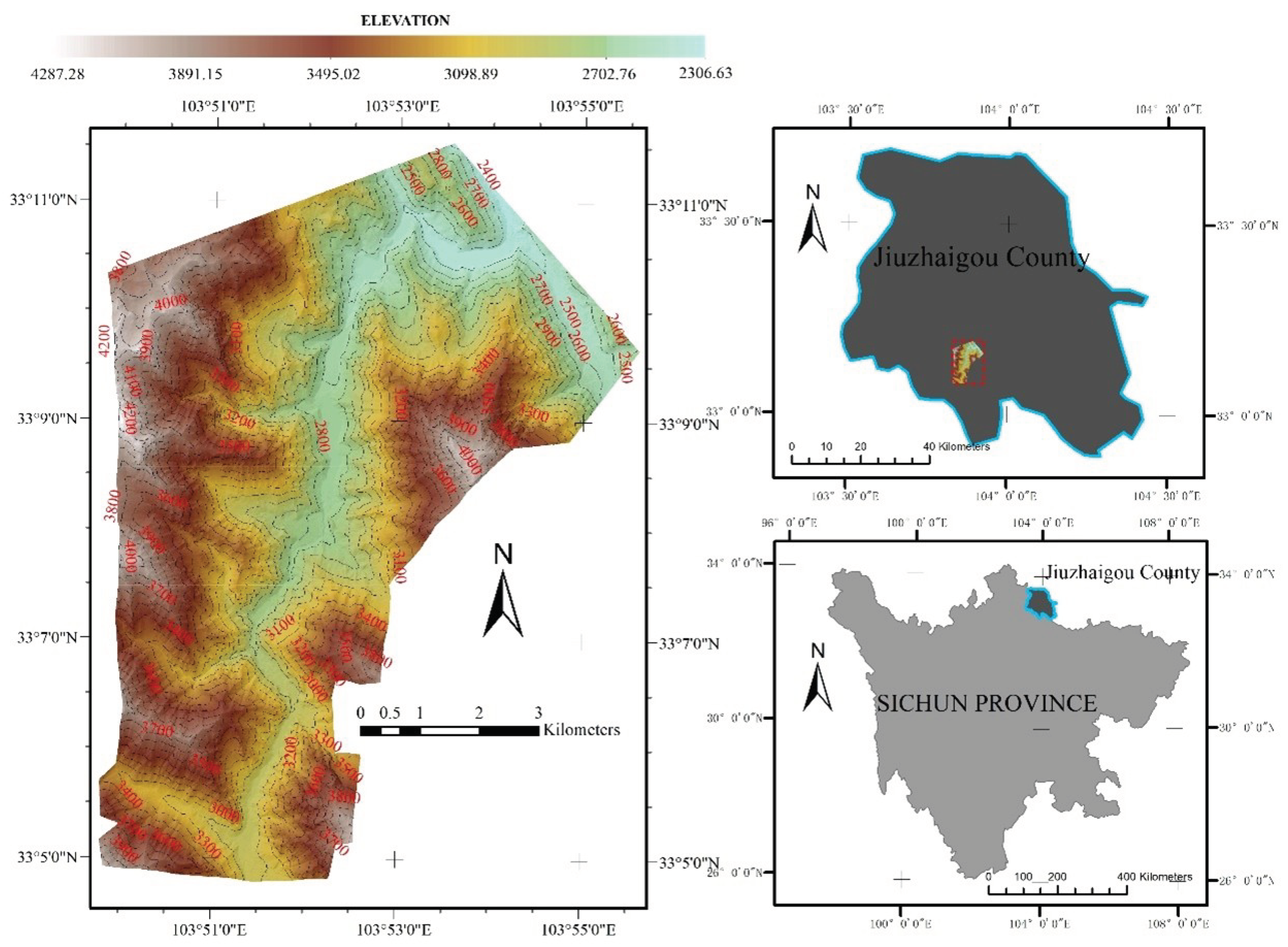
Figure 3.
Three representative regions were selected for illustration. From left to right: column(a) shows the original point cloud, column(b) shows the ground truth DEM, column(c) shows the DEM generated by our method, column(d) shows the DEM produced by linear interpolation, and column(e) shows the DEM produced by nearest-neighbor interpolation.
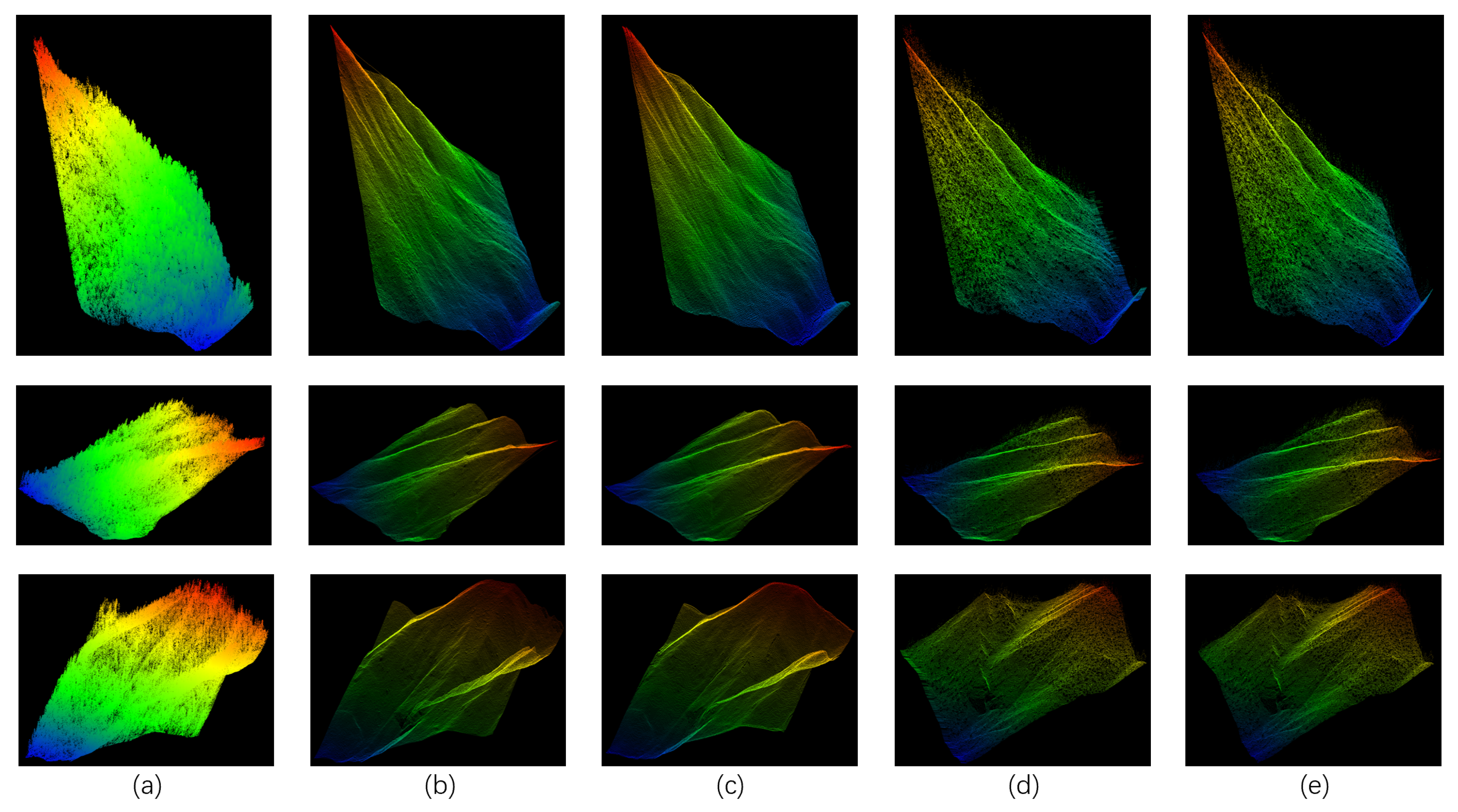
Figure 4.
Comprehensive visualization of error distribution patterns and magnitude details for both nearest neighbor and linear interpolation methodologies applied to DEM reconstruction. This detailed error analysis clearly reveals the spatial distribution of reconstruction inaccuracies, highlighting areas where traditional interpolation methods fail to capture terrain complexity and produce significant elevation discrepancies.
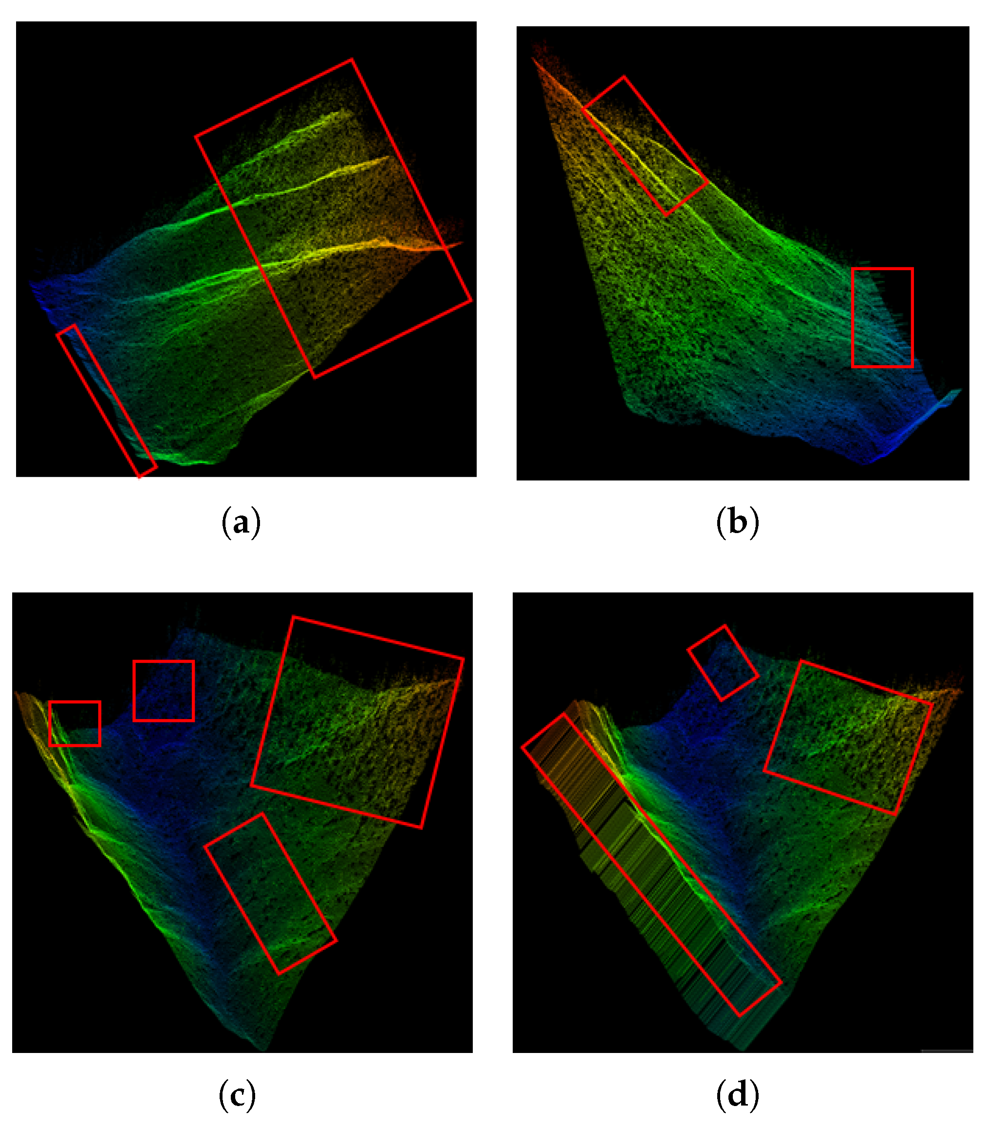
Figure 5.
The detailed visualization of the high-resolution DEM generated through the application of our proposed methodological approach. This comprehensive visual representation clearly demonstrates the superior spatial accuracy and terrain reconstruction fidelity achieved by our innovative processing framework. The resulting DEM exhibits exceptional preservation of fine-scale topographic features while maintaining smooth surface continuity across complex terrain morphology.
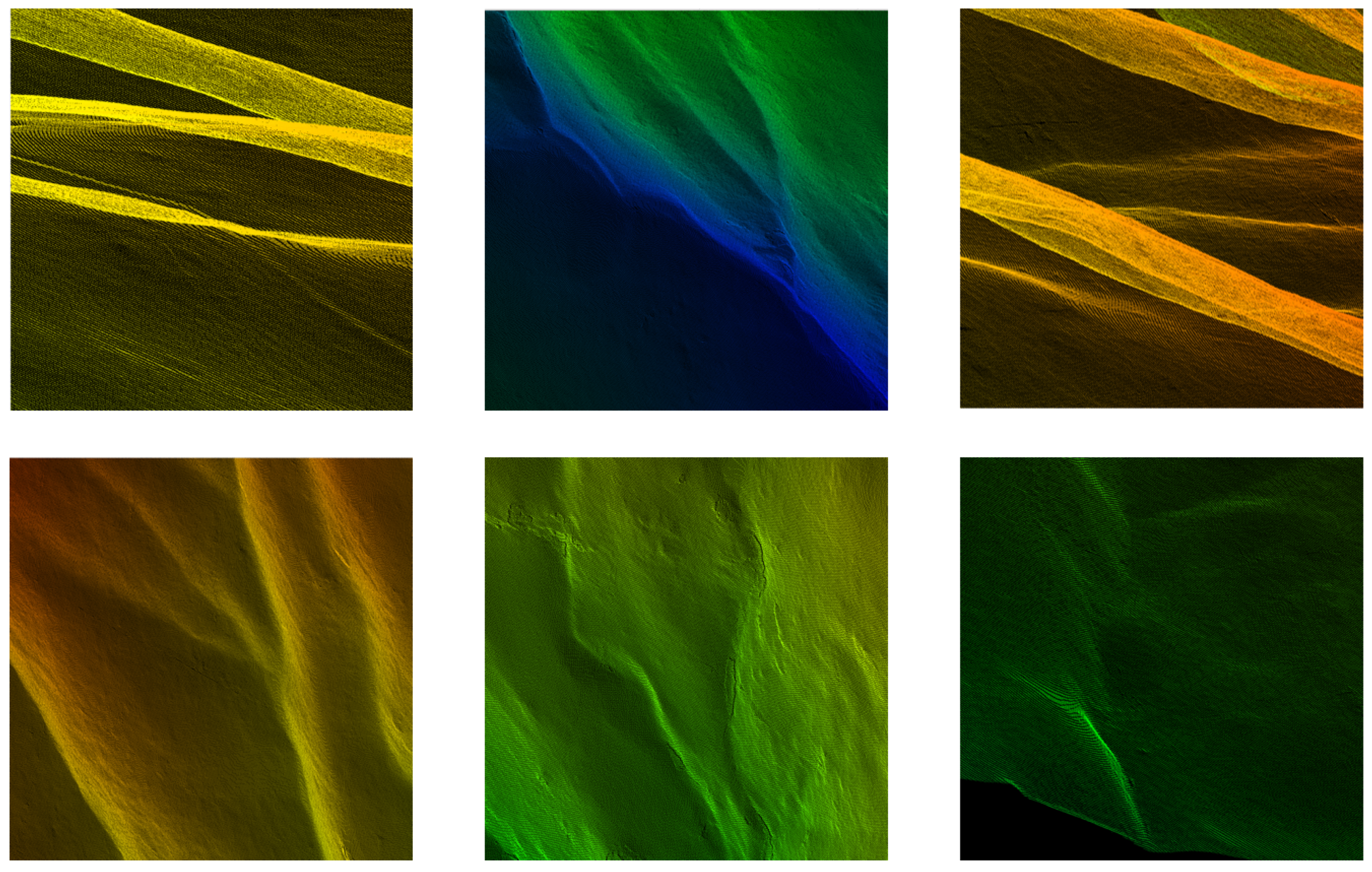
Table 2.
Quantitative Accuracy Assessment of DEMs
| Experiment | Method | RMSE | MAE |
|---|---|---|---|
| Ours | 1.30 | 0.77 | |
| Experiment 1 | Linear | 121.81 | 103.29 |
| Nearest | 121.37 | 102.69 | |
| Ours | 1.06 | 0.71 | |
| Experiment 2 | Linear | 110.48 | 90.50 |
| Nearest | 109.06 | 88.80 |
Table 3.
Processing Time Analysis for Different DEM Generation Approaches
| Methods | Ours | Nearest | Linear |
|---|---|---|---|
| Experiment 1 | 7.62s | 11.82s | 14.05s |
| Experiment 2 | 6.86s | 9.14s | 11.47s |
Disclaimer/Publisher’s Note: The statements, opinions and data contained in all publications are solely those of the individual author(s) and contributor(s) and not of MDPI and/or the editor(s). MDPI and/or the editor(s) disclaim responsibility for any injury to people or property resulting from any ideas, methods, instructions or products referred to in the content. |
© 2025 by the authors. Licensee MDPI, Basel, Switzerland. This article is an open access article distributed under the terms and conditions of the Creative Commons Attribution (CC BY) license (http://creativecommons.org/licenses/by/4.0/).
Copyright: This open access article is published under a Creative Commons CC BY 4.0 license, which permit the free download, distribution, and reuse, provided that the author and preprint are cited in any reuse.


