Submitted:
12 June 2025
Posted:
13 June 2025
You are already at the latest version
Abstract
This paper discusses the degradation of two types of highly porous insulating firebricks under monotonic and cyclic loadings in uniaxial compression. Strain-controlled cyclic fatigue tests were performed with either constant strain limit or constant strain amplitude. Damage indicators are based on stress-strain data and impulse excitation technique. When the strain limit/amplitude was below the maximal strain of linear proportion of the materials, no damage was induced. This criterion was used to compare damage formation in the materials. In cyclic tests with constant strain limit, damage stagnated in the second phase of fatigue and no failure occurred. In cyclic tests with constant strain amplitude, the greater the strain amplitude, the lower the number of cycles the samples resisted before the failure. Damping was found a more sensitive damage indicator with higher variations than E modulus. Prediction of the damage state in the materials was possible with irreversible strain and dissipated energy data.
Keywords:
dissipated energy
; ladle lining
; life time
; thermal strain
; ceramics
1. Introduction
Insulating firebricks (IFB) are refractory ceramics based on lightweight aggregates. Since 1930s they have been used in the construction of high temperature vessels. In the multi-layer structure of steel ladle, IFBs are employed as safety lining between the ladle’s shell and working lining to conserve heat and protect ladle’s shell from experiencing extreme temperatures. As IFBs possess low bulk density and low thermal conductivity. However, IFBs suffer from low mechanical properties due to highly porous (>45%) microstructure. In literature decrease in physical and mechanical properties in terms of elastic modulus [1,2,3], bending strength [4,5], compressive strength [6,7] and fracture toughness [4,5,8] with an increase of porosity is well-documented. Traon et al. [3] measured dynamic Young’s modulus, damping and ultra sound velocity of several alumina castables with porosity ranges of 19%-32%. They found dynamic Young’s modulus, damping and travelling time changed by around -60%, +350% and +145% in samples with the highest level of porosity (32%) in comparison to the samples with the lowest level of porosity (19%), respectively [3]. Meille et al. [6] investigated uniaxial compression behavior of alumina ceramics with porosity ranges of 30%-75%. They reported a decrease of compressive strength and its coefficient of variation by the increase of the pore volume fraction. In terms of pore size, the fracture strength was greater by 63%-68% in highly porous samples (>50%) with small pores (<125 µm) as compared to the ones with large pores (224 µm – 355 µm). They witnessed brittle fracture and a rather cellular like fracture for relative porosity below and above 50%, respectively. The compressive behavior in the former and latter groups was mainly controlled by the presence of isolated pores and distribution of the solid phase, respectively [6].
The temperature fluctuations due to the cyclic nature of batch production exposes IFBs to repetitive thermomechanical loads. For this, IFBs are repeatedly squeezed between the two stiffer layers of working lining and ladle’s shell. A spike in loads or multiple lower intensity loads make IFBs prone to instant or gradual failure. The failure of IFBs destabilizes the working lining. Consequently, studying monotonic and cyclic compressive fatigue behavior of IFBs is vital for material selection purposes and potentially contributes to development of superior IFB products. Several studies investigated cyclic fatigue degradation of relatively dense refractories (porosity < 23%) in uniaxial compression [9,10,11,12], bending [12,13,14,15,16], tension [17,18] and wedge splitting [19,20,21,22] in strain-controlled or stress-controlled setups. No studies on cyclic fatigue degradation of highly porous refractories is known to the authors. Limited studies [23,24] addressed (mechanical) cyclic fatigue response of porous ceramics. Yonezu et al. [23] investigated static and cyclic fatigue strength of SiC and Cordierite ceramics with porosities of 37% and 30% in four point bending setup, respectively. They found degradation of fracture strength was controlled by static fatigue (time dependent) and the cyclic component of loading had no impact on the strength of their samples [23]. Miyazaki et al. [24] studied cyclic fatigue behavior of alumina ceramics with porosities of 0.8%, 35% and 47% in three point bending setup. For all three series of samples, they observed an increase of life distribution with the decrease of applied (maximal) stress, similar to metallic materials. When they normalized the applied stress for each series, they noted longer life (number of cycles to failure) for porous series than the dense alumina at similar (normalized) stress levels. Their fractographic analysis revealed the crack blunting and stress relaxation impact of pores at the crack tip. They also noted crack propagation was easier when the pore’s density and diameter were greater. Both factors shortened fatigue life of their samples [24].
Overload fracture occurs in monotonic loading test, however cyclic (fatigue) loading test may not necessarily lead to failure. It mostly involves a degradation process with various rates depending on the fatigue phase. The degradation process is quantified by monitoring the alteration of irreversible strain [9,16,20], strain rate, compliance [12,21] and (strain) dissipated energy [20,26] based on stress-strain data. The input energy is lower in cyclic loading than monotonic loading [20], however the energy absorption capacity is greater resulting in crack branching and a wider fracture process zone. The energy dissipation capacity is attributed to microstructural characteristics of the developed fracture process zone [20]. In addition, non-destructive provide complimentary insights into the degradation process. Acoustic emission [15,16,17] and ultra sound velocity [11] measurements enable localization of damage. AE could quantify limits of critical loads based on the extent of damage [16]. Dynamic Young’s modulus [14,15] and damping data obtained by impulse excitation could potentially indicate the onset and accumulation of damage globally alike the mentioned techniques. However seldom applied as criteria of cyclic fatigue on refractories.
In the present work, degradation of two types of commercially available IFBs under monotonic and cyclic fatigue loadings was studied. The tests were conducted in uniaxial compression setup. Strain-controlled cyclic tests were performed with either constant strain (upper) limits or constant strain amplitudes. The methods are based on two possible load scenarios taking place in service [12]. Fatigue degradation was analyzed using damage indicators based on stress-strain data, including compliance, irreversible strain, strain rate and dissipated energy, and a non-destructive method called impulse excitation including dynamic Young’s modulus and damping. The discussion contributes in extending understanding of materials degradation process in service along with the limits and advantages of the employed damage indicators.
2. Materials and Methods
Two commercially available IFBs from high alumina products were studied in as-received state. IFB 26 belongs to ASTM group 26 with service limit temperature of 1430 ⁰C (2600 ⁰F). IFB 28 belongs to ASTM group 28 with service limit temperature of 1530 ⁰C (2800 ⁰F). The classification is based on the maximum allowed application temperature and the bricks are generally fired up to these temperatures during their production. The detailed chemical and physical properties of the studied materials are addressed in the Results section of the paper. The typical microstructure of the materials is shown in Figure 1.
The chemical and mineralogical composition of the powdered samples were characterized using XRF and XRD (Rietveld) techniques, respectively. For XRF a PW2404 device (Malvern PANalytical BV) was used, whereas for XRD a Bruker D8 Advance with LynxEye detector (Bruker AXS), CuKα tube and Kβ nickel filter working at 40 kV and 40 mA were employed. The XRD patterns were recorded in range of 5⁰–90⁰ (2Θ), using a step size of n.d. 0.01⁰ and a step rate of 0.5 s. TOPAS software package for Rietveld refinement was used for semi-quantitative determination of phase proportions. The refinement was done on the assumption of pure phases. Microstructural investigations were performed with a LEO Type 440i (Leo Electron Microscopy) scanning electron microscope (SEM). For estimation of total porosity (P), the following equation was used:
where ρb is the bulk density (mass/volume) and ρt is the true density, measured using a helium pycnometer (Ultrapyc-1200e, Quantachrome).
Monotonic and cyclic loading tests were conducted in uni-axial compression setup at room temperature with an Instron 1186 mechanical test frame. The loading rate was 0.3mm/min. The width, height and length of the samples were 30 mm, 60 mm and 230 mm, respectively. The samples faces were polished to ensure their plane-parallelity. The strain was calculated as the ratio of recorded displacement over the initial height of the sample. Cyclic tests were performed in displacement-controlled setup, as refractories in service are predominantly exposed to strain-controlled loads which result from thermal expansion of the involved materials [12,25]. Two types of cyclic tests, as of method II and method III described in [12], were performed. In the loading protocol of method II slight modification was applied by introducing a minimal force level for the end of unloading to avoid decoupling of the sample and the loading piston. Nevertheless, both of the methods are briefly explained here. For method II, a constant displacement limit was defined as the upper limit of the loading cycles and for the lower limits of the cycles where unloading stops a minimal force of 500 N was introduced. The next cycle starts when the minimal force limit was attained. In method II the upper limit is fixed regardless of the developed damage, whereas in method III the upper limit is not fixed but the cycle amplitude is. In method III loading proceeds till a constant displacement amplitude is reached for every cycle regardless of the developed damage. In method III the unloading, alike method II, stops at a minimal force level of 500 N. The next cycle starts where the former unloading met the minimal force level. The main characteristics of method II and method III are constant displacement (upper) limit and constant displacement amplitude, respectively. For all the cyclic tests irreversible strain of every cycle was calculated at the minimal force level after correction of displacement. Cyclic tests of method II were performed on IFB 28 material and strain limit was in the range of 25%-160% of the registered strain at maximal stress of monotonic loading curves. Cyclic tests of method III were conducted on both of the materials. The strain amplitudes were in the range of 18%-75% and 50%-160% of the registered strain at maximal stress of monotonic loading curves of IFB 26 and IFB 28, respectively. The maximal number of cycles for the cyclic tests was set to 250 cycles. In cyclic tests of method III, the cycle proceeding to total strain of 10% was assumed as the final cycle. For this, the failure criteria was set to total strain of 10%.
For estimation of the dissipated energy, the surface area under the unloading curve was deduced from the surface area below the loading curve of stress-strain data [26]. The dissipated energy was determined for a specific number of cycles from each cyclic test. For calculation of strain rate, the produced irreversible strain in every cycle was divided by that cycle’s duration. For all cycles of every cyclic test, strain rate was calculated. For calculation of compliance, the change of strain was divided by the change of stress at 30% and 70% of the maximal stress reached in the cycle. For all cycles of every cyclic test the compliance was calculated. The compliance is the inverse of stiffness, modulus of elasticity. For certain cycles also modulus of elasticity was calculated.
The dynamic Young’s (E) modulus and damping were obtained at room temperature by the impulse excitation technique with a Resonant Frequency Damping Analyzer (RFDA) from IMCE BV. The measurements were conducted on the samples before applying load (as-received state), after the first cycle and after the last cycle. The last cycle was only feasible on the samples which did not experience complete failure. The approach of evaluating the resultant damage of the cyclic tests by measuring the change of E modulus was previously reported effective by [9,10,16] due to its non-destructive nature.
3. Result and Discussion
3.1. Microstructural Characterization
The chemical and physical properties of the materials are addressed in Table 1. The materials have similar constituents, but the quantities vary between them. IFB 28 has a higher amount of alumina but lower amount of silica and impurities (K2O, Fe2O3 and TiO2) than IFB 26. Both materials constitute moderate levels of amorphous content. The main crystalline phases are mullite (3Al2O3∙2SiO2) and corundum (Al2O3), meanwhile very low amounts of quartz and cristobalite were also identified in the samples. The amount of quartz is expected to be slightly higher in IFB 26 than IFB 28. Both materials have a similar level of porosity (around 73%). The bulk and true density of IFB 28 are higher than IFB 26 by around 13% and 10%, respectively. The microstructure of the materials is mainly composed of fine grains and pores, in contrast to the microstructure of dense refractories where large grains (aggregates in millimeter-scale) are frequent. Instead, pores and cavities (dark background - resin-filled, Figure 1) are dominant. Alumina grains mainly have a porous structure sometimes with a Si-containing edge. The elemental composition of the edges suggests presence of traces of various impurities, including but not limited to alkalis like, K2O and Na2O (Figure 1-c and d). Quartz particles are not as frequent as alumina but, wherever they are found in the microstructure, they have an Al-containing edge and are accompanied with an aluminosilicate composite (Figure 1-c). This composite consists of dense, hair-like and randomly oriented grains in a dense matrix. The size of these grains is too small to be accurately analyzed with EDS, but possibly could be mullite which has nucleated and grown from an Al-rich siliceous matrix, as has been previously reported by [27].
3.2. Monotonic Loading Tests
Force-displacement curves of monotonic loading tests is shown in Figure 2. The parameters were extracted and briefed in Table 2. The compressive strength of IFB 28 is higher than IFB 26 by around 30%. In IFB 28 the maximal stress was reached just after the linear proportion, but in case of IFB 26 the stress falls and rises again after the linear proportion. For this, the coefficient of variation is higher in IFB 26 than IFB 28 with respect to maximal stresses. In terms of strain, failure occurs at lower values in IFB 28 than IFB 26, in fact the strain at maximal stress of IFB 28 is lower than IFB 26 by 54%. However, when linear proportion is considered, the maximal strain of linear proportion is higher by 47% in IFB 28 than IFB 26. This means IFB 28 has a higher elastic strain tolerance than IFB 26. The characteristics of linear proportion in the materials will be used later in the discussion of cyclic fatigue results. The modulus of elasticity shows IFB 28 is stiffer than IFB 26 (by around 18%). One when compares the stress-strain curves (Figure 2) with similar curves of relatively dense refractories studied in [11,12], can note in the former no sudden failure occurs. This, as described by [6], is due to continuous failure of the solid structure around the pores.
Measurement of damping reflects the ability of the material to absorb and dissipate mechanical energy [28]. The damping values of ceramics lie in the range of 10-6-10-1, as reported by [28,29]. According to [30] damping values measured via the impulse excitation technique are reliable in the range of approximately 10-5-10-1, the values greater than 0.1 are not very reliable due to the influence of external friction sources. In as-received state, before conducting cyclic measurements, dynamic Young’s modulus and damping properties of all samples in two directions, low thickness (s) and high thickness (l) were measured. Figure 3 shows the correlation of damping and dynamic Young’s modulus for both directions. As it can be seen, damping correlates indirectly with dynamic Young’s modulus, meaning the sample with higher dynamic Young’s modulus possess lower damping and vice versa. Similar correlation is reported in [31] when the degradation of alumina castables due to thermal shock was investigated. In order to correlate dynamic Young’s modulus of samples in as-received state with modulus of elasticity estimated based on the data of the first cycle, Figure 4 was depicted. Despite scatter, for both materials dynamic Young’s modulus correlates directly with modulus of elasticity.
3.3. Cyclic Loading Tests
Stress-strain curves of two medium intensity cyclic tests of method II and III are shown as examples in Figure 5. For the former the strain limit is 0.48% and for the latter the strain amplitude is 0.4%. In method III (Figure 5-b), the development of every cycle follows the stress-strain envelope of the sample. One can clearly distinct the pre-peak, peak and post peak area. While in method II (Figure 5-a), peak and post-peak areas may not develop. As strain at maximal stress and strain of linear proportion (SNLP) of IFB 28 are 0.6%, 0.44%, respectively, one can expect the peak stress in case of sample of method II is reached. However, as the upper limits strain in method II is constant, the post peak part of the envelope is not developed. Unlike the example of method II, the presence of a well-developed post peak area is obvious in the example of method III.
From stress-strain curves of Figure 5 several parameters were extracted and are shown distinctly in two series of graphs for each method’s example (Figure 6). The parameters are strain (Figure 6-a,b), stress (Figure 6-c,d) and cycle’s duration (Figure 6-e,f) with respect to the number of cycles. This was done to show the evolution of each parameter in the lower and upper limits of every cycle. Comparing the evolution of strain at the limits in method II and method III examples, one can note the evolution of strain in method III shows three phases of fatigue degradation. Strain initially sharply increases, then the rate of changes calms shortly (phase II) and follows by an exponential increase up to failure (phase III). Whereas in case of method II’s example only the first two phases of fatigue were witnessed. Strain initially increases exponentially (phase I) but shortly after, the rate of increase stagnates and becomes almost constant (phase II). The difference becomes more obvious to the eyes by comparing the change of strain (black) curves. Even though the upper limits strain is growing in method III’s example, in case of method II it was kept constant (Figure 6-a,b). Evolution of stress in upper limits follows a different trend in method II and method III. In method III, the stress increases in the first few cycles (positive values) whereas in method II stress of only the second cycle (yellow dot) may be higher than the first cycle and then it starts to decrease. Change of stress in every consecutive cycle (black curves - Figure 6-c,d) becomes almost constant and remain negative. As the extent of damage is more significant in example of method III than method II, one can note the closeness of upper and lowers stresses (red dots – Figure 6-c,d) in method III than method II. In terms of cycle’s duration examples of method II and method III could be compared. In general, it follows a similar trend as of upper stress limits. In method II, second cycle is longest cycle where the highest stress was recorded. After the first few cycles, the cycles become abruptly shorter (phase I) and then the rate tends to slow down, but keeps decreasing in case of method II (incomplete phase II). In case of method III, the first few cycles become lengthier (phase I) and then almost constant during phase II. With the start of phase III, the cycles become gradually shorter. By comparison of the position of black and red dots in Figure 6-e,f, one can note that the duration of the last cycle in method II is significantly lower than the first cycle, whereas in case of method III the difference is less (5 s, 7%).The consecutive cycles in the cyclic tests of method II become consistently shorter as the accumulated strain gets closer to the defined strain limit, but in the cyclic tests of method III strain grows and accumulates with the cycles up to the failure.
The maximal stress (SIG) every first cycle reached and its modulus of elasticity (ME) are depicted in Figure 7. It can be noted with the increase of strain amplitude/limit the corresponding first cycle reaches a higher SIG value. The SIG values approach peak stress values obtained from monotonic tests, especially for strain amplitudes/limits close and above SNLP limit of the materials. It can be seen for similar strain amplitudes, IFB 28 samples reached higher SIG values than IFB 26 samples. This is in line with lower peak stress of IFB 26 than IFB 28 obtained from monotonic loading tests. Unlike SIG, ME of the first cycles with respect to strain amplitude/limit do not show any specific trend, rather mostly scatter within the range of ME values obtained from monotonic loading tests.
3.4. Damage Indicators and Degradation Process
The evolution of damage in the materials could be compared in terms of compliance (Figure 8-a,b,c), irreversible strain (Figure 9-a,b,c), strain rate (Figure 10-a,b,c) and dissipated energy (Figure 11-Figure 12) between method II and method III. As only IFB 28 was tested in method II and method III, the material comparison would be limited to method III results and methods comparison would be limited to IFB 28 results.
Figure 8.
Evolution of compliance with number of cycles in cyclic tests of method II (a) and method III, IFB28(b) and IFB26(c), SL-strain limit and SA-strain amplitude.
Figure 8.
Evolution of compliance with number of cycles in cyclic tests of method II (a) and method III, IFB28(b) and IFB26(c), SL-strain limit and SA-strain amplitude.
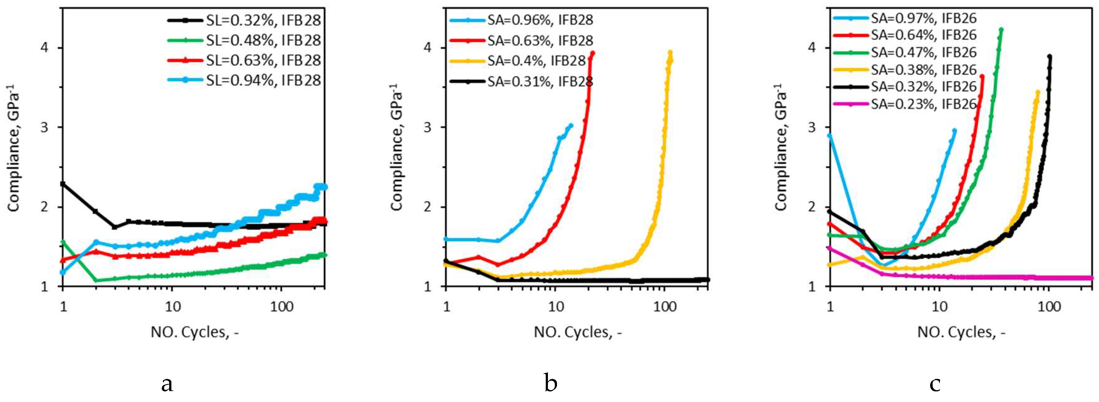
Figure 9.
Evolution of irreversible strain with number of cycles in cyclic tests of method II (a) and method III, IFB28(b) and IFB26(c), SL-strain limit and SA-strain amplitude.
Figure 9.
Evolution of irreversible strain with number of cycles in cyclic tests of method II (a) and method III, IFB28(b) and IFB26(c), SL-strain limit and SA-strain amplitude.
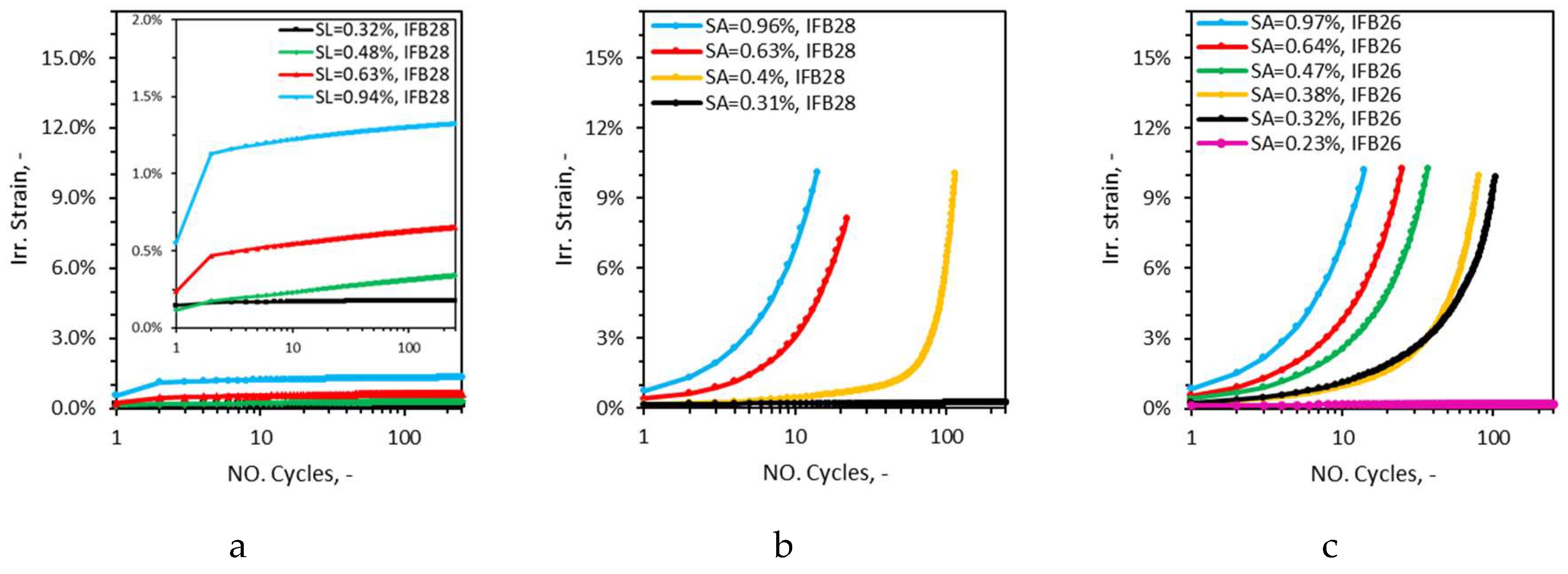
Figure 10.
Evolution of strain rate with number of cycles in cyclic tests of method II (a) and method III, IFB28(b) and IFB26(c), SL-strain limit and SA-strain amplitude.
Figure 10.
Evolution of strain rate with number of cycles in cyclic tests of method II (a) and method III, IFB28(b) and IFB26(c), SL-strain limit and SA-strain amplitude.
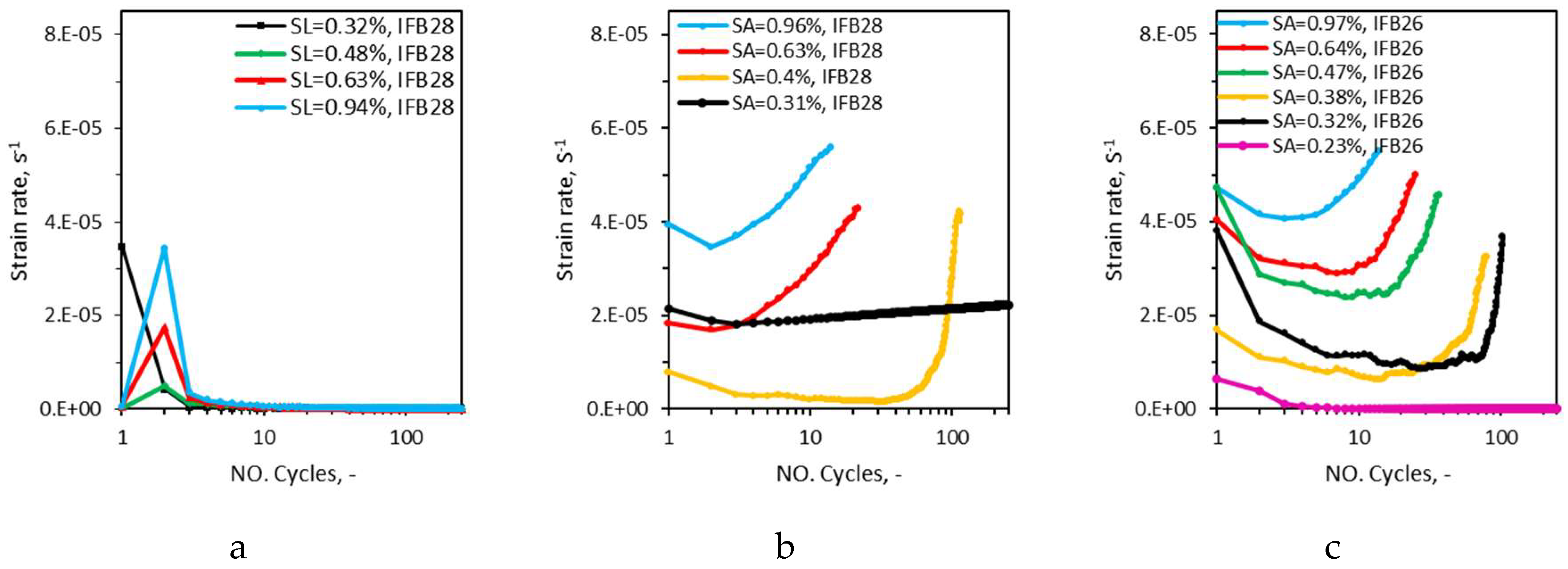
Figure 11.
Evolution of dissipated energy with number of cycles in cyclic tests of method II, SL-strain limit.
Figure 11.
Evolution of dissipated energy with number of cycles in cyclic tests of method II, SL-strain limit.
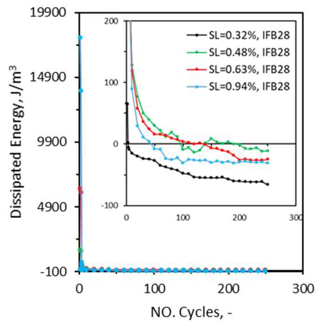
Figure 12.
Evolution of dissipated energy with number of cycles in cyclic tests of method III, low (a), medium (b) and high (c) strain amplitudes, SA-strain amplitude.
Figure 12.
Evolution of dissipated energy with number of cycles in cyclic tests of method III, low (a), medium (b) and high (c) strain amplitudes, SA-strain amplitude.
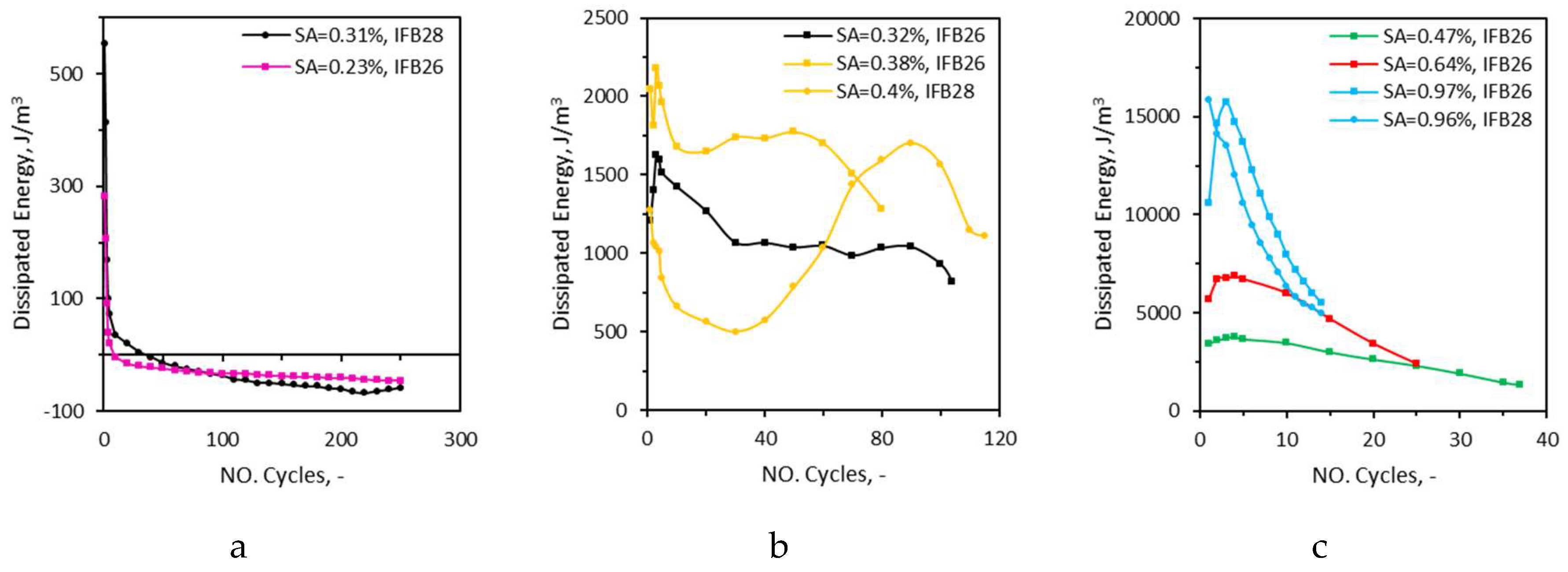
In case of method III, compliance and strain rate curves form a bath-tub shape, whereas in case of method II, as the third phase of fatigue is not developed, the last part of the tub shape (exponential increase) is replaced by a rather steady line. In case of method III, irreversible strain forms an exponential shape, however again as the third phase of fatigue is not developed in method II, after the second cycle irreversible strain forms a line with a slightly increasing slope. The slope of the line increases in every case with the increase of strain limit. The black curve, which had strain limit of 0.32%, shows almost no degradation, after the second cycle all three parameters stay constant throughout the measurement. The blue curve presents the steepest increase among all curves which has a strain limit of 0.94%. In case of method III curves also colours are representative of a similar magnitude of strain amplitude, instead of strain limits. In case of method III curves, the blue curves do not necessarily have the steepest slope, but rather shifted toward the left of the plot. As with increasing strain amplitude, the second phase of fatigue becomes shorter, earlier (in terms of number of cycles) the exponential increase (phase III) kicks off. The black curve remains steady with no (limited) sign of damage. However, the black curve, which has strain amplitude of 0.32% in the case of IFB 26 demonstrate fatigue degradation which was not the case for IFB 28. This can be explained by recalling the strain of linear proportion (SNLP) of the materials. The strain amplitude of the black curve 0.31% is lower than the SNLP of IFB 28 (0.44%) but higher than SNLP of IFB 26 (0.30%). The pink curve, which has strain amplitude of 0.23% develops no damage throughout the measurement again as its strain amplitude is lower than SNLP of IFB 26.
When the loading and unloading curves fully overlap, the energy put into the sample is recovered after removal of the load and sample returns to its original state. Otherwise, the energy is lost in the form of heat or damage in the sample [32]. During cyclic loading the dissipated energy by heat stays almost constant [33]. For this, the change in dissipated energy in consecutive cycles is related to the degradation of the sample [26]. A crack within the microstructure would only propagate, if there is a change in the dissipated energy of two consecutive cycles [34]. The extent of degradation is higher when more energy is dissipated in a cycle. Figure 11 and Figure 12 show the evolution of dissipated energy in cyclic tests of method II and method III, respectively. In all cyclic tests of method II, the trend is as follows: The dissipated energy starts with a relatively high magnitude, but abruptly drops to negative values after just a few cycles. Then the rate of decrease stagnates until the final cycle. Here the negative values of dissipated energy mean that the unloading curve had overlapped the loading one and no energy was dissipated. This observation is in line with the other damage indicators where damage was produced only during the first few cycles in cyclic tests of method II. The low intensity (strain amplitude) tests conducted in method III setup (Figure 12-a) follow a similar trend as of the curves of the cyclic tests of method II (Figure 11). Here again only during the first few cycles some energy (but to a much lower extent than medium and high strain limit tests of method II) is dissipated. Unlike the low intensity curves, medium (Figure 12-b) and high (Figure 12-c) strain amplitude curves of cyclic tests method III do not approach negative values. Even they are different in terms of profile shape. In medium intensity strain amplitude tests the initial decrease of dissipated energy is followed by an increasing trend before decreasing again up to failure. The curve has a s-shape in the case of the sample of IFB 28 which was cycled at strain amplitude of 0.4%. In case of IFB 26 materials, the magnitude of dissipated energy initially increases, then decreases up to failure. The initial increase of dissipated energy can be attributed to the occurrence of strain hardening due to compaction in this material. However, such behaviour was not witnessed for the samples of IFB 28. The rate of decrease of dissipated energy increased with the increase of strain amplitude in both of the materials.
Figure 13 and Figure 14 present changes of modulus of elasticity (ME) and upper limits stress (SIG) for the second and last cycles in comparison to the first cycle for all cyclic measurements, respectively. For the measurements performed at the strain amplitude of 0.23%, 0.31% as they were below the SNLP of their respective material, the values of the SIG and ME for both the second and last cycles are all positive, except for method II in which the ME of last cycle for the sample cycled at 0.32% is negative. In case of method III, these samples experienced stiffening through the cycles without loss of stress capacity. For the same strain limit, 0.32%, the sample lost its stiffness by -46%. For all samples cycled at strain amplitude/limit above their respective SNLP, the values of SIG and ME of last cycles lie in the negative range. This is in line with the fact that the samples went through degradation. In case of IFB 28 a similar trend applies to the second cycles, but this is not the case for IFB 26. It can be seen that black triangles are all positive irrespective of the applied strain amplitude (Figure 14-b). This implies IFB 26 in method III went through strain hardening, even though the first cycle could have well-passed the material’s SNLP limit.
The change of dissipated energy in the second and last cycles in comparison to the first cycle of the cyclic tests of method II and method III are depicted in Figure 15-a and Figure 15-b, respectively. In case of no failure samples, the dissipated energy of the last cycle is lower by 100%-200% than the first cycle’s dissipated energy. For samples cycled with strain amplitudes in the range of SNLP of the materials the difference of dissipated energy between the first and last cycle becomes minimal. In IFB 26 sample which was cycled at the strain amplitude of 0.32%, the difference is only -32%. In IFB 28 sample which was cycled at the strain amplitude of 0.4%, the difference of dissipated energy of the last and first cycle is only -13%. For higher strain amplitudes the difference becomes in the range of 48%-68%. In IFB 26 samples, the dissipated energy in the most of the cases was higher in the second cycles than the first cycles. As mentioned earlier, possibly the strain hardening due to the compaction of the material explains such behaviour.
Figure 16 and Figure 17 present the changes of damping and dynamic Young’s modulus of samples after the first and 250th (last) cycles in comparison to their original state, respectively. Two directions, the low thickness (s) and high thickness (l) were employed to address precisely the damage on the sides of the samples. As it can be seen from the figures, the general trend is with the increase in extent of damage, damping values (logarithmic scale) increase, while the dynamic Young’s modulus decreases. The magnitude of changes in damping are much higher than dynamic Young’s modulus. For the sample cycled at the strain limit of 0.97%, after 250 cycles El corresponds to -56.2% while Dl shows 2831%. Damping seems to be the more sensitive damage indicator than the dynamic Young’s modulus. For the sample cycles at 0.32% strain limit, neither dynamic Young’s modulus nor irreversible strain (Figure 18) indicate any development of damage, but damping parameters after 250 cycles are 11% (Ds), 22% (Dl). The magnitude of changes of dynamic Young’s modulus is similar for IFB 28 samples after the first cycle where strain amplitude and limit were similar, however the damping differs significantly. The higher scatter in damping data after the first cycles requires more datapoints to obtain a more reasonable data fit. For low and medium intensity strain amplitudes, both damping and dynamic Young’s modulus show higher extent of damage (changes) in IFB 26 than IFB 28 after the first cycle, but for high intensity strain amplitudes data is not consistent. In IFB 26, with the increase of strain amplitude not necessarily the changes of dynamic Young’s modulus and damping increases, the low value of goodness of linear fit for this material, unlike IFB 28 can be noted from Figure 17 and Figure 16.
The data of all samples after the first and 250th cycles was linearly fitted, the equation and the goodness of fit are shown. In case of irreversible strain, as the data for the second cycle was also available, the same was done. The goodness of fit for damping curves is slightly lower which can be attributed to the sensitivity of the method. The irreversible strain developed with respect to strain amplitude/limit is depicted in Figure 18 for the first, second and last cycle (method II only). As it can be seen, with the increase of strain amplitude/limit, the developed irreversible strain increases. For IFB 28 samples cycled at strain amplitude/limit of 0.3% almost no irreversible strain was developed as the amplitude/limit was below the materials respective SNLP limit. The further the amplitude/limit gets from SNLP limits, greater irreversible strain is developed. Interestingly the amount of irreversible strain developed by the samples cycled at the same strain amplitude/limit in method II and method III are similar. The samples cycled at the strain amplitude/limit of 0.63% and 0.96% in method II and method III develop around 0.23% and 0.55% irreversible strain, respectively. This is due to the fact that the only similarity in terms of cycle setup method II and method III share is the first cycle and the consecutive cycles follow different paths. For low and medium intensity strain limits, the irreversible strain produced after the last cycle is in the range of the second cycle. For high intensity strain limits, the amount of irreversible strain produced after the last cycle is by 20%-45% greater than the irreversible strain recorded after the second cycle, which is a very small development in comparison to irreversible strain developed after the last cycle in method III. From Figure 22 It can be also inferred for similar strain amplitudes IFB 26 samples developed a greater amount of irreversible strain than IFB 28 after the first cycle. At strain amplitude of 0.3% IFB 28 developed only 0.04% irreversible strain whereas IFB 26 sample developed 0.12% irreversible strain.
For the prediction of damage trend in the last cycle of the cyclic tests of method III, dissipated energy was the only feasible parameter. Irreversible strain was not helpful since the total strain of 10% was assumed as the failure criteria for cyclic tests of method III. Measurements of dynamic Young’s modulus and damping property were not possible due to the sever extent of damage (failure of samples). Figure 19 shows the energy dissipated by sample after the first, second and last cycles of cyclic tests. For similar strain limits and amplitudes, the magnitude of dissipated energy is close for the first and second cycles but quite different for the last cycle. The samples cycled at the strain limit of 0.94% and strain amplitude of 0.96% dissipated around 1700 J/m3 and 1400 J/m3 energy during the first and second cycles, but during the last cycle the former and latter dissipated -30 J/m3 and 5000 J/m3, respectively. Summing up the amount of dissipated energy during the first and second cycle, it can be noted in low and medium intensity strain amplitudes, IFB26 dissipated greater amount of energy than IFB 28 but in case of high intensity strain amplitudes the values become close and even greater for IFB 28.
The strain of proportional limit (SNLP) obtained from monotonic loading tests was found to define the potential for failure of the samples in cyclic tests of method III. For the studied materials, especially in case of IFB 26 strain at maximal stress was found unsatisfactory for this purpose. The cyclic tests conducted with strain amplitude below SNLP of the material did not result in failure (Figure 20). The cyclic tests with strain amplitude greater than the defined SNLP of the materials ended with the failure of the sample. For this, IFB 28 shows sensitivity to damage formation at higher strains than IFB 26. The greater the strain amplitude the lower the number of cycles the sample sustained before failure. Method III permits build-up of damage, enables comparison of the degradation process in the materials.
Method II represents the constrained thermal expansion occurring in service. For this, in practice as long as the loads (thermal strains) are within the elastic limits of the IFBs, no degradation occurs. By increase of the load magnitude over the elastic limits, compaction of the IFBs occur. This may initially lead to some relaxation as the degradation process stagnates with no major crack formation. In the framework of the current study, however none of the samples tested in the cyclic method II setup failed. None of the damage indicators showed the third phase of fatigue for the cyclic tests of method II, even though the strain limit in case of high intensity tests was well above the defined SNLP of the material. Similar to the tests of repetitive thermal cycles [35], damage tended to stagnate in the cyclic test of method II for the number of cycles investigated in this study. Potentially for a higher number of cycles in tests of high intensities failure may occur.
4. Conclusions
The materials did not show sign of degradation when the applied strain limit/amplitude was below the maximal strain of their linear proportion. IFB 28 showed sensitivity to fatigue failure at higher strain amplitudes than IFB 26. In the first few cycles IFB 26 showed strain hardening possibly due to compaction irrespective of the applied strain amplitude. The greater the strain amplitude, the lower the number of cycles the samples sustained before failure. For the studied strain limits, no complete failure occurred in samples tested in method II setup. In all tests of method II damage stagnated in the second phase of fatigue and the third phase of fatigue did not develop. The same happened for low intensity (strain amplitude) tests of method III. The degradation patterns and trends were more different between the methods than between the materials. The rate of degradation intensifies with the increase of strain amplitudes for compliance, irreversible strain, strain rate curves, but in case of dissipated energy the shape of curve profiles changes. All damage indicators consistently presented formation and propagation of damage in the samples with the increase of number of cycles. Damping and dynamic Young’s modulus data of IFB 26 did not show a linear increase of damage extent with the increase of strain amplitude, but irreversible strain and dissipated energy data did. Damping was found to be the more sensitive damage indicator than the dynamic Young’s modulus with the highest magnitude of variation. However, damage indicators based on stress-strain data can be continuously measured and more easily accessible without the need for decoupling the sample from the testing machine. This allows prediction of extent of fatigue damage (in terms of irreversible strain and dissipated energy) in the materials up to failure.
Acknowledgments
The work was supported during 2018-2021 by the funding scheme of the European Commission, Marie Skłodowska-Curie Actions Innovative Training Networks in the frame of the H2020 European project ATHOR - Advanced THermomechanical multiscale mOdelling of Refractory linings - 764987 Grant. Ralf Coenen is thanked for SEM measurements.
References
- R. L. COBLE and W. D. KINGERY, “Effect of Porosity on Physical Properties of Sintered Alumina,” J. Am. Ceram. Soc., vol. 39, no. 11, pp. 377–385, Nov. 1956. [CrossRef]
- W. Pabst, E. Gregorová, and G. Tichá, “Elasticity of porous ceramics - A critical study of modulus-porosity relations,” J. Eur. Ceram. Soc., vol. 26, no. 7, 2006. [CrossRef]
- N. Traon, T. Tonnesen, R. Telle, B. Myszka, and R. Silva, “Influence of the Pore Shape on the Internal Friction of Refractory Castables,” in Proceedings of the Unified International Technical Conference on Refractories (UNITECR 2013), Hoboken, NJ, USA: John Wiley & Sons, Inc., 2014, pp. 141–146.
- García-Prieto, M. Dos Ramos-Lotito, D. Gutiérrez-Campos, P. Pena, and C. Baudín, “Influence of microstructural characteristics on fracture toughness of refractory materials,” J. Eur. Ceram. Soc., vol. 35, no. 6, pp. 1955–1970, Jun. 2015. [CrossRef]
- N. Miyazaki and T. Hoshide, “Influence of Porosity and Pore Distributions on Strength Properties of Porous Alumina,” J. Mater. Eng. Perform., vol. 27, no. 8, pp. 4345–4354, Aug. 2018. [CrossRef]
- S. Meille, M. Lombardi, J. Chevalier, and L. Montanaro, “Mechanical properties of porous ceramics in compression: On the transition between elastic, brittle, and cellular behavior,” J. Eur. Ceram. Soc., vol. 32, no. 15, 2012. [CrossRef]
- E. Ryshkewitch, “Compression strength of porous sintered alumina and zirconia,” J. Am. Ceram. Soc., vol. 36, no. 2, pp. 65–68, 1953. [CrossRef]
- R. W. Rice, “Grain size and porosity dependence of ceramic fracture energy and toughness at 22°C,” J. Mater. Sci., vol. 31, no. 8, pp. 1969–1983, 1996. [CrossRef]
- Y. Hino and Y. Kiyota, “Fatigue Failure and Thermal Spalling Tests to Evaluate Dynamic Fatigue Fracture of MgO–C Bricks,” ISIJ Int., vol. 51, no. 11, pp. 1809–1818, 2011. [CrossRef]
- Y. Hino and Y. Kiyota, “Fatigue Failure Behavior of Al2O3-SiO2 System Bricks under Compressive Stress at Room and High Temperatures,” ISIJ Int., vol. 52, no. 6, pp. 1045–1053, 2012. [CrossRef]
- K. Andreev, M. Boursin, A. Laurent, E. Zinngrebe, P. Put, and S. Sinnema, “Compressive fatigue behaviour of refractories with carbonaceous binders,” J. Eur. Ceram. Soc., vol. 34, no. 2, pp. 523–531, 2014. [CrossRef]
- K. Andreev, V. Tadaion, J. Koster, and E. Verstrynge, “Cyclic fatigue of silica refractories – effect of test method on failure process,” J. Eur. Ceram. Soc., vol. 37, no. 4, pp. 1811–1819, 2017. [CrossRef]
- Y. Hino, K. Yoshida, Y. Kiyota, and M. Kuwayama, “Fracture Mechanics Investigation of MgO-C Bricks for Steelmaking by Bending and Fatigue Failure Tests Along with X-Ray CT Scan Observation,” Tetsu-to-Hagane, vol. 100, no. 11, pp. 1371–1379, 2014. [CrossRef]
- K. Andreev, V. Tadaion, Q. Zhu, W. Wang, Y. Yin, and T. Tonnesen, “Thermal and mechanical cyclic tests and fracture mechanics parameters as indicators of thermal shock resistance – case study on silica refractories,” J. Eur. Ceram. Soc., vol. 39, no. 4, 2019. [CrossRef]
- K. Andreev, N. Shetty, and E. Verstrynge, “Acoustic emission based damage limits and their correlation with fatigue resistance of refractory masonry,” Constr. Build. Mater., vol. 165, pp. 639–646, 2018. [CrossRef]
- K. Andreev, N. Shetty, M. de Smedt, Y. Yin, and E. Verstrynge, “Correlation of damage after first cycle with overall fatigue resistance of refractory castable concrete,” Constr. Build. Mater., vol. 206, 2019. [CrossRef]
- F. Thummen, C. Olagnon, and N. Godin, “Cyclic fatigue and lifetime of a concrete refractory,” J. Eur. Ceram. Soc., vol. 26, no. 15, pp. 3357–3363, 2006. [CrossRef]
- M. Ghassemi Kakroudi, M. Huger, C. Gault, and T. Chotard, “Damage evaluation of two alumina refractory castables,” J. Eur. Ceram. Soc., vol. 29, no. 11, 2009. [CrossRef]
- K. Andreev, B. Luchini, M. J. Rodrigues, and J. L. Alves, “Role of fatigue in damage development of refractories under thermal shock loads of different intensity,” Ceram. Int., vol. 46, no. 13, 2020. [CrossRef]
- K. Andreev, Y. Yin, B. Luchini, and I. Sabirov, “Failure of refractory masonry material under monotonic and cyclic loading – Crack propagation analysis,” Constr. Build. Mater., vol. 299, 2021. [CrossRef]
- Y. Dai, D. Gruber, and H. Harmuth, “Determination of the fracture behaviour of MgO-refractories using multi-cycle wedge splitting test and digital image correlation,” J. Eur. Ceram. Soc., vol. 37, no. 15, pp. 5035–5043, Dec. 2017. [CrossRef]
- Y. Dai, Y. Li, S. Jin, H. Harmuth, and X. Xu, “Fracture behavior of magnesia refractory materials under combined cyclic thermal shock and mechanical loading conditions,” J. Am. Ceram. Soc., vol. 103, no. 3, 2020. [CrossRef]
- Yonezu, T. Ogawa, and H. Kawamoto, “Fatigue strength and fracture mechanisms of porous ceramics,” Mater. Sci. Res. Int., vol. 8, no. 3 SPEC., 2002. [CrossRef]
- N. Miyazaki, T. Hoshide, and K. Kikukawa, “Life Properties and Effect of Pore-Characteristics in Fatigue of Porous Alumina,” in 13th International Conference on the Mechanical Behaviour of Materials (ICM13), 2019, pp. 437–445.
- C. A. Schacht, Refractory linings: Thermomechanical design and applications. CRC Press, 2017.
- Z. Song, T. Frühwirt, and H. Konietzky, “Characteristics of dissipated energy of concrete subjected to cyclic loading,” Constr. Build. Mater., vol. 168, 2018. [CrossRef]
- D. J. Duval, S. H. Risbud, and J. F. Shackelford, “Mullite,” Ceram. Glas. Mater. Struct. Prop. Process., pp. 27–39, 2008. [CrossRef]
- E. Gregorová, W. Pabst, P. Diblíková, and V. Nečina, “Temperature dependence of damping in silica refractories measured via the impulse excitation technique,” Ceram. Int., vol. 44, no. 7, pp. 8363–8373, 2018. [CrossRef]
- J. Zhang, R. J. Perez, and E. J. Lavernia, “Documentation of damping capacity of metallic, ceramic and metal-matrix composite materials,” J. Mater. Sci., vol. 28, no. 9, pp. 2395–2404, May 1993. [CrossRef]
- G. Roebben, B. Bollen, A. Brebels, J. Van Humbeeck, and O. Van Der Biest, “Impulse excitation apparatus to measure resonant frequencies, elastic moduli, and internal friction at room and high temperature,” aip.scitation.org, vol. 68, no. 12, p. 4511, 1997. [CrossRef]
- T. Tonnesen and R. Telle, “Thermal shock damage in castables: Microstructural changes and evaluation by a damping method.,” Ceram. forum Int., vol. 84, no. 9, pp. E1–E5, 2007.
- K. A. Ghuzlan and S. H. Carpenter, “Fatigue damage analysis in asphalt concrete mixtures using the dissipated energy approach,” Can. J. Civ. Eng., vol. 33, no. 7, pp. 890–901, Jul. 2006. [CrossRef]
- V. Dattoma and S. Giancane, “Evaluation of energy of fatigue damage into GFRC through digital image correlation and thermography,” Compos. Part B Eng., no. 47, pp. 283–289, 2013, Accessed: Oct. 07, 2022. [Online]. Available online: https://www.sciencedirect.com/science/article/pii/S1359836812007287.
- S. Shen, G. D. Airey, S. H. Carpenter, and H. Huang, “A dissipated energy approach to fatigue evaluation,” Road Mater. Pavement Des., vol. 7, no. 1, pp. 47–69, Jan. 2006. [CrossRef]
- E. D. Case, “The saturation of thermomechanical fatigue in brittle materials.,” in Thermomechanical Fatigue and Fracture, Southampton, UK: WIT Press, 2002, pp. 137–208.
Figure 1.
SEM micrographs of the studied IFBs in as received state - IFB-26 (a, b - zoomed) and IFB-28 (c, d - zoomed). Inserted numbers in micrographs are addressing the following substances: 1 - alumina, 2 - an aluminosilicate composite and 3 - silica.
Figure 1.
SEM micrographs of the studied IFBs in as received state - IFB-26 (a, b - zoomed) and IFB-28 (c, d - zoomed). Inserted numbers in micrographs are addressing the following substances: 1 - alumina, 2 - an aluminosilicate composite and 3 - silica.
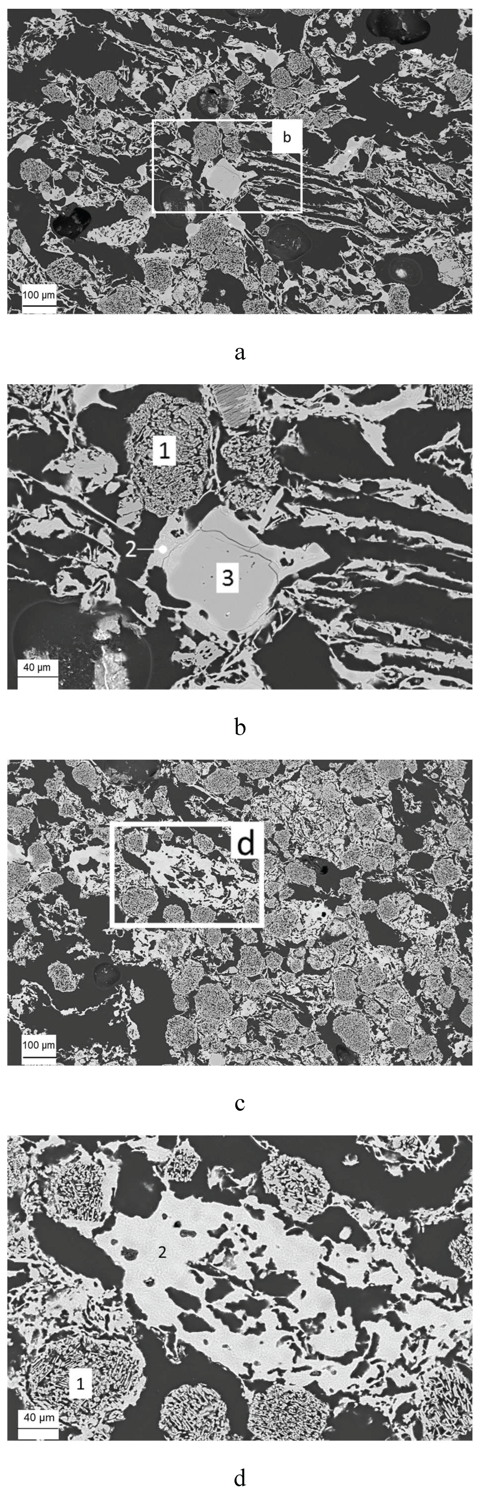
Figure 2.
Force-displacement curves of IFB 26 (a) and IFB 28 (b) obtained from monotonic compressive loading tests.
Figure 2.
Force-displacement curves of IFB 26 (a) and IFB 28 (b) obtained from monotonic compressive loading tests.
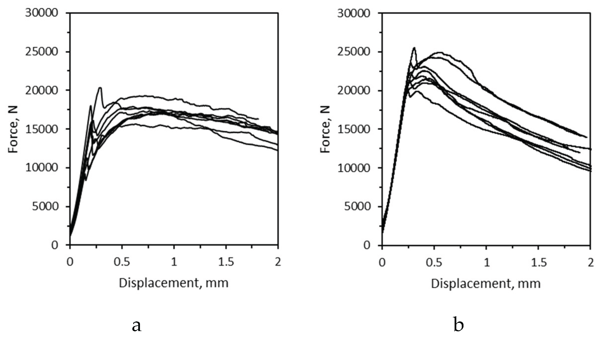
Figure 3.
Correlation of damping (D) and dynamic Young’s modulus (E) data in IFB 26 and IFB 28 samples used in cyclic (CYC) measurements before applying loads measured in two directions, s- short thickness(a) and l- high thickness(b).
Figure 3.
Correlation of damping (D) and dynamic Young’s modulus (E) data in IFB 26 and IFB 28 samples used in cyclic (CYC) measurements before applying loads measured in two directions, s- short thickness(a) and l- high thickness(b).
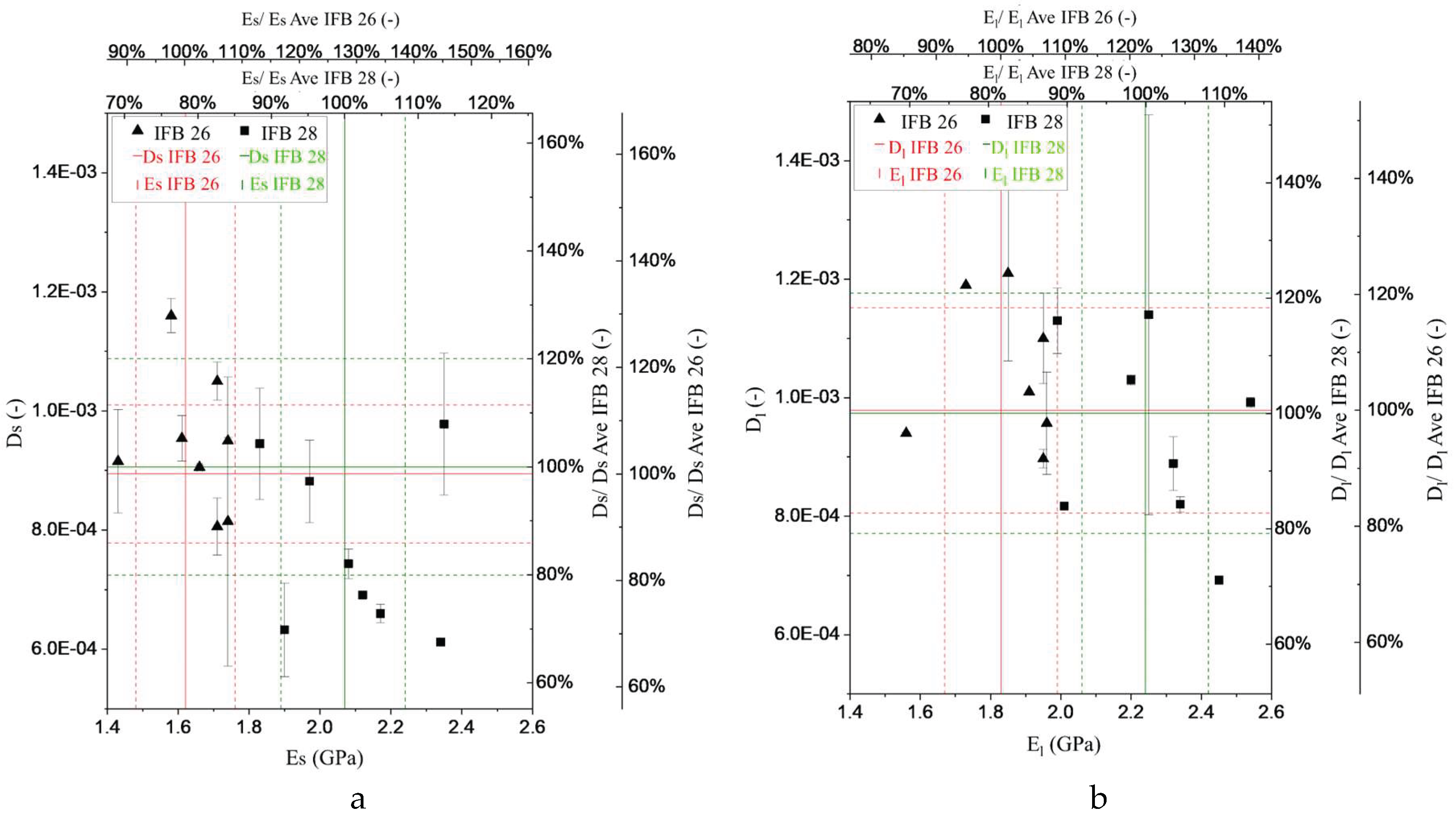
Figure 4.
Correlation of modulus of elasticity (ME) and dynamic Young’s modulus (E) of IFB 26 and IFB 28 samples used in cyclic (CYC) measurements in two directions, s- short thickness(a) and l- high thickness(b). MON data obtained from monotonic loading tests. Full line average value and dashed line a standard deviation.
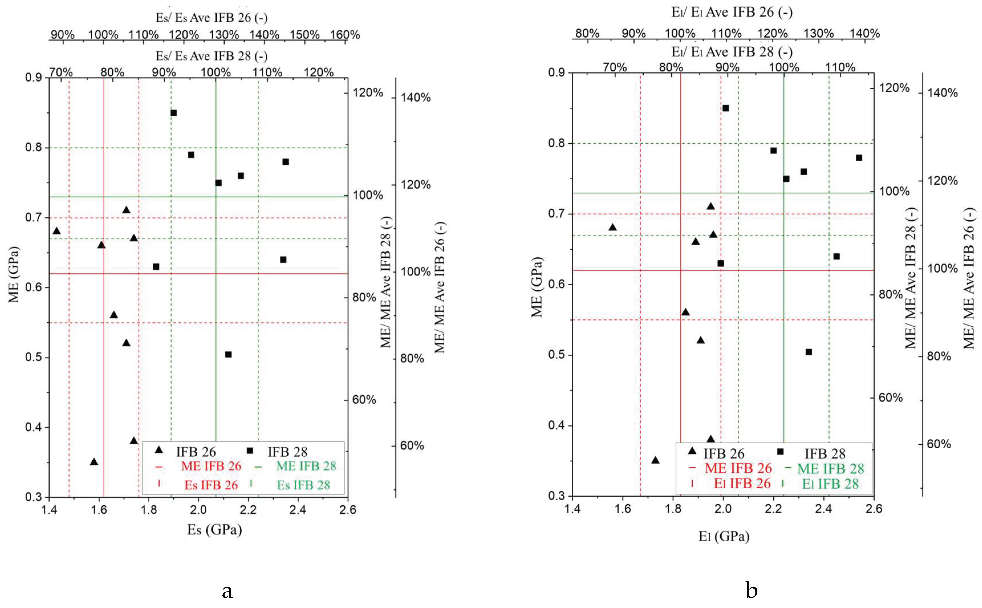
Figure 5.
Example of cyclic fatigue methods – a stress-strain curve of method II (a) and method III (b). First, second and last cycles are drawn in black, yellow and red, respectively.
Figure 5.
Example of cyclic fatigue methods – a stress-strain curve of method II (a) and method III (b). First, second and last cycles are drawn in black, yellow and red, respectively.
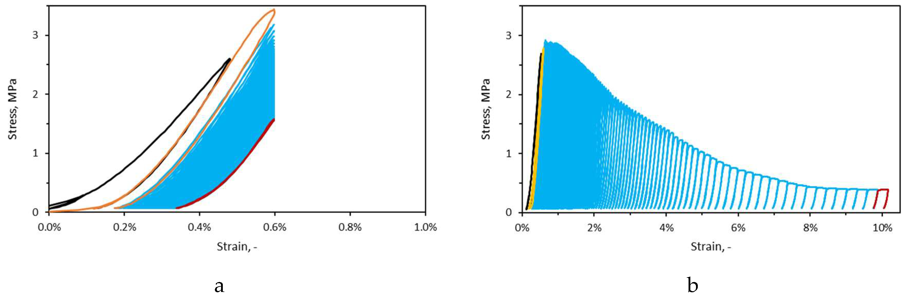
Figure 6.
Evolution of strain (a,b), stress (c,d) and cycles duration (e,f) with respect to number of cycles. a,c,e and b,d,f were extracted from the curves of Figure 9-a (method II) and Figure 9-b (method III), respectively.
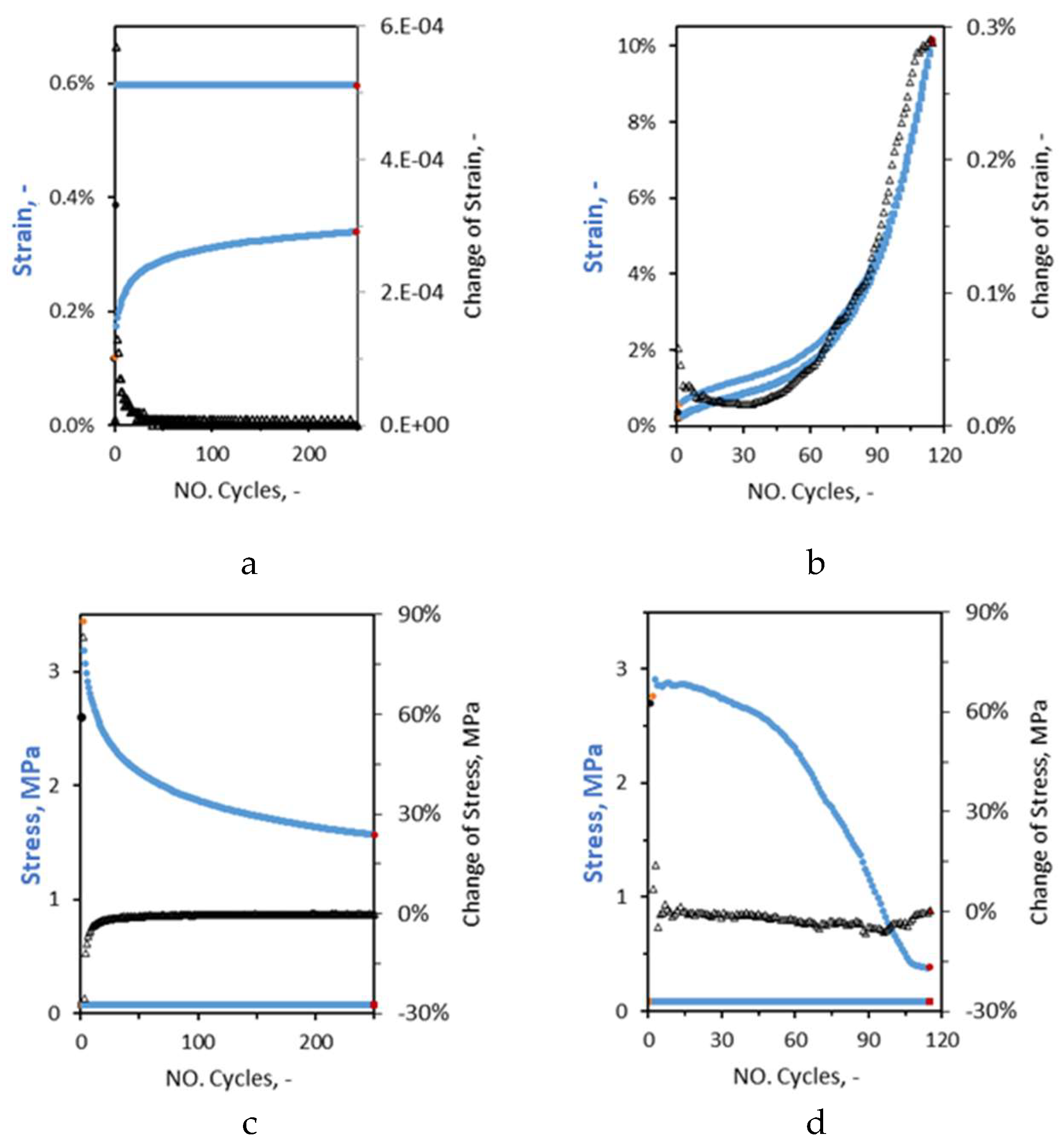
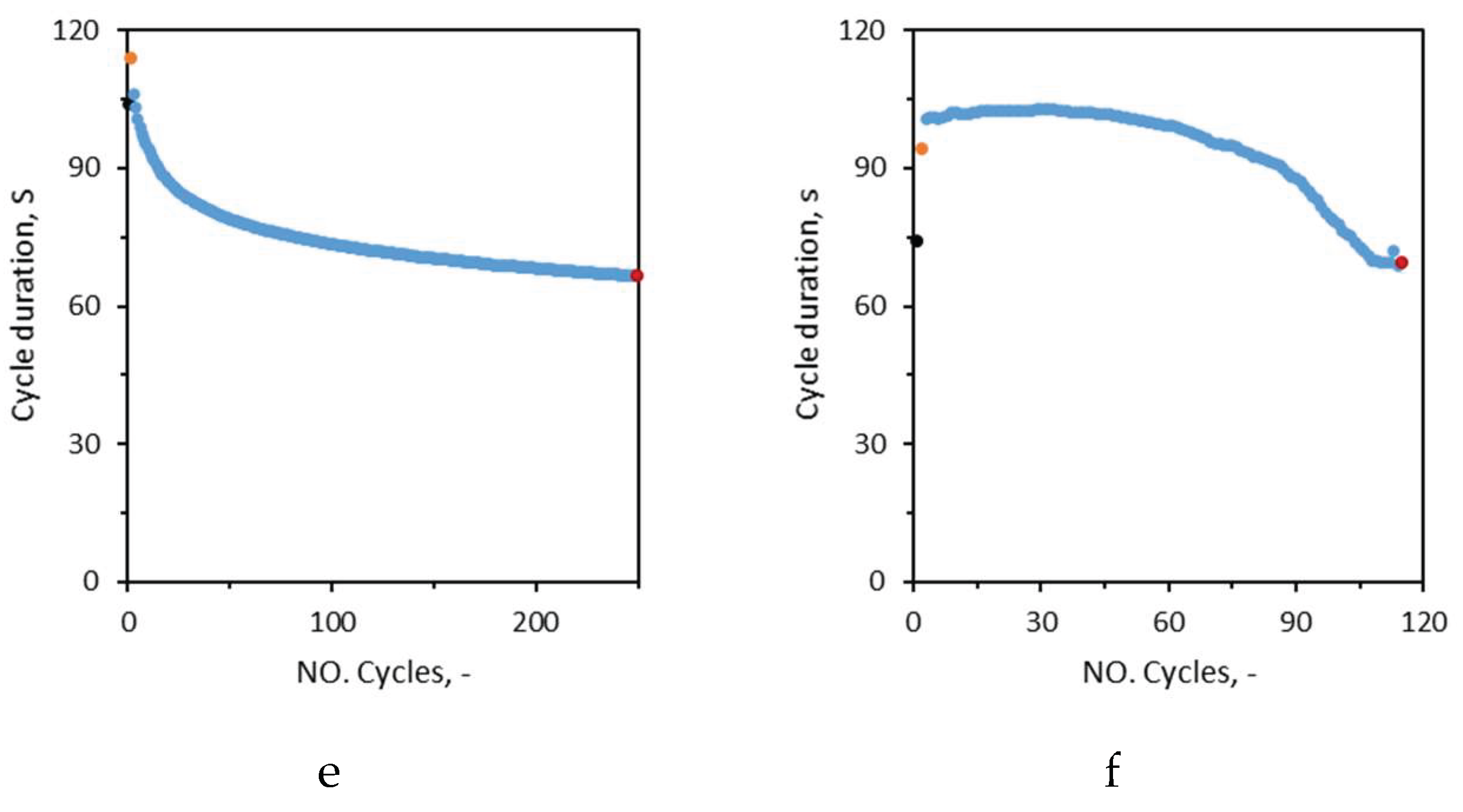
Figure 7.
Maximal stress-SIG(a) and modulus of elasticity-ME(b) achieved after the first cycle.
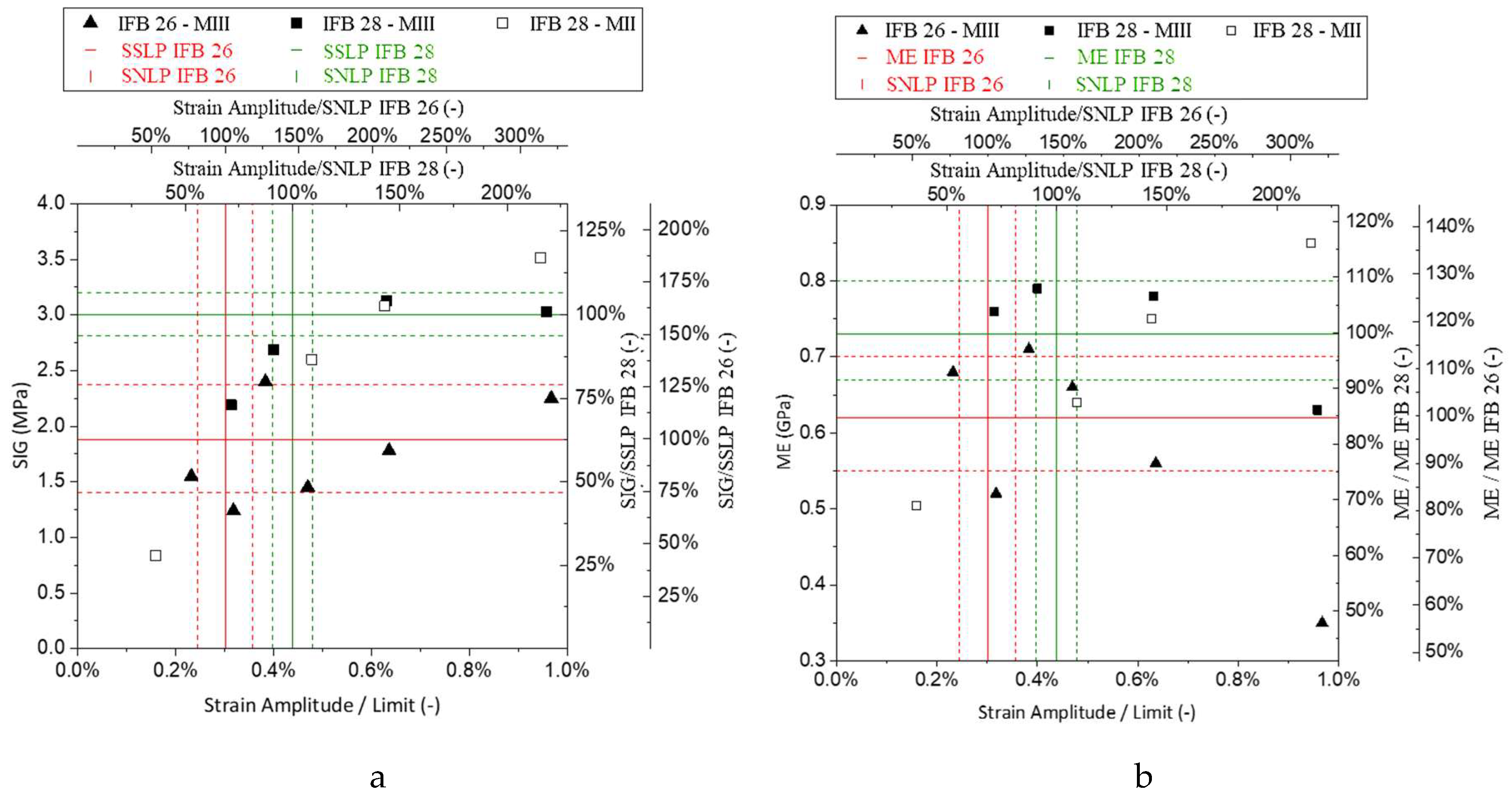
Figure 13.
Change of modulus of elasticity (ME) in the second and last cycle in comparison to the first cycle in cyclic tests of method II (a) and method III(b).
Figure 13.
Change of modulus of elasticity (ME) in the second and last cycle in comparison to the first cycle in cyclic tests of method II (a) and method III(b).
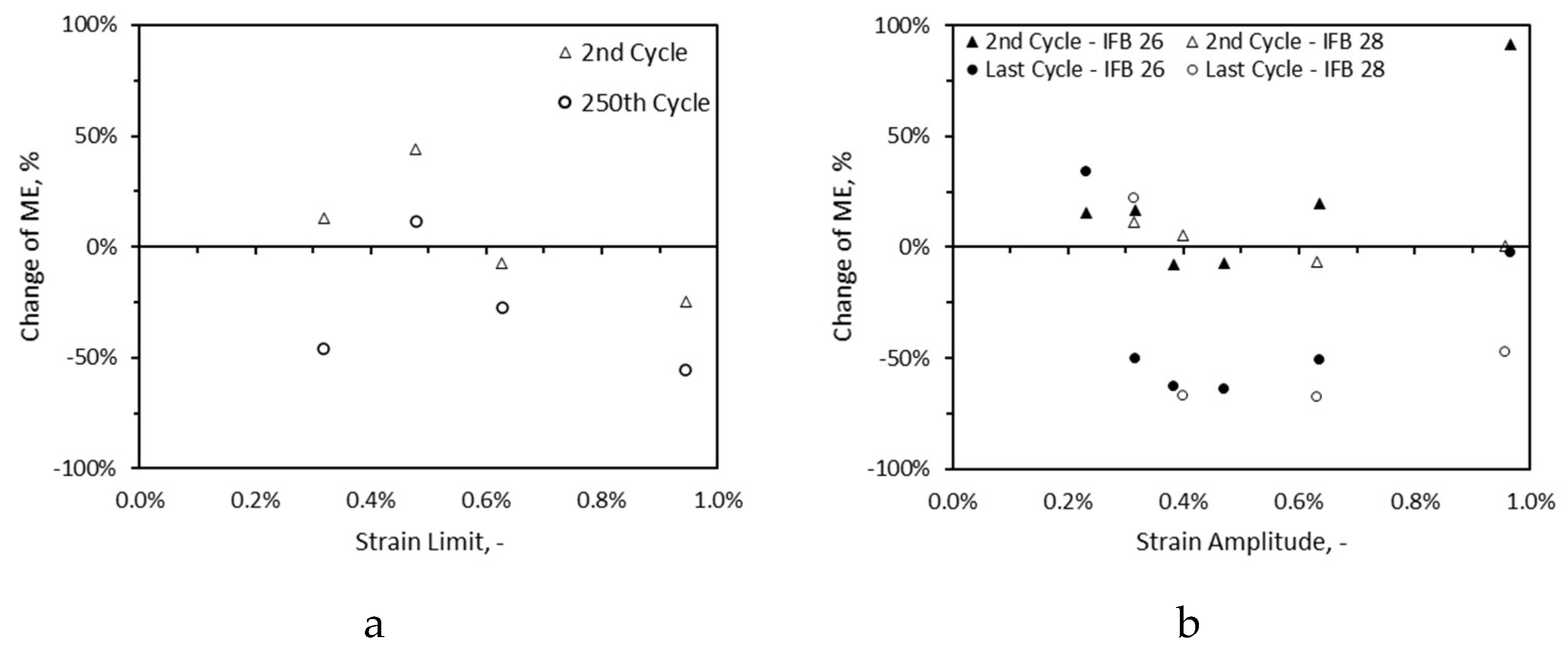
Figure 14.
Change of maximal stress (SIG) in the second and last cycle in comparison to the first cycle in cyclic tests of method II (a) and method III(b).
Figure 14.
Change of maximal stress (SIG) in the second and last cycle in comparison to the first cycle in cyclic tests of method II (a) and method III(b).
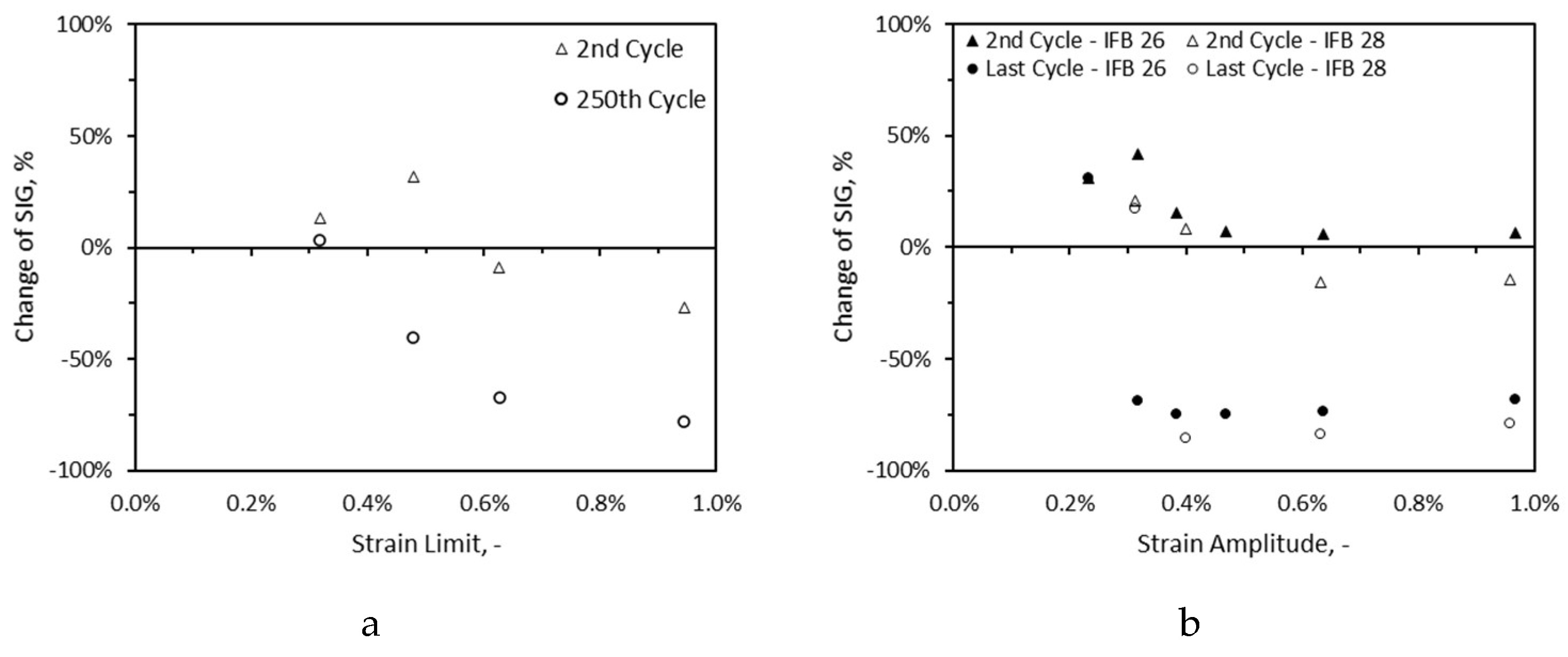
Figure 15.
Change of dissipated energy in the second and last cycle in comparison to the first cycle in cyclic tests of method II (a) and method III(b).
Figure 15.
Change of dissipated energy in the second and last cycle in comparison to the first cycle in cyclic tests of method II (a) and method III(b).
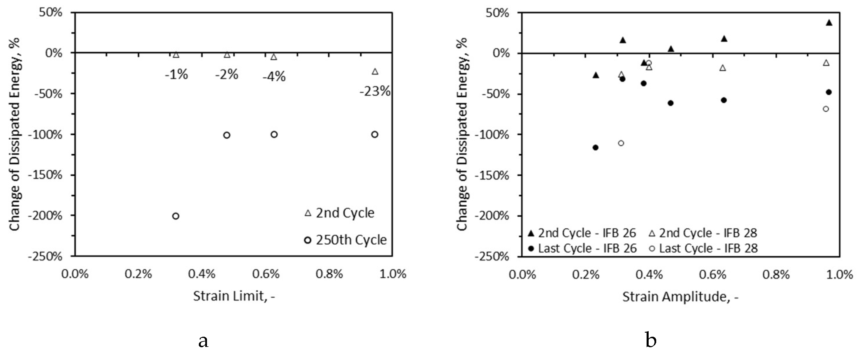
Figure 16.
Damage trends based on change of damping in cyclic tests of method II (a) and method III (b).
Figure 16.
Damage trends based on change of damping in cyclic tests of method II (a) and method III (b).

Figure 17.
Damage trends based on change of dynamic Young’s modulus (E modulus) in cyclic tests of method II (a) and method III (b).
Figure 17.
Damage trends based on change of dynamic Young’s modulus (E modulus) in cyclic tests of method II (a) and method III (b).
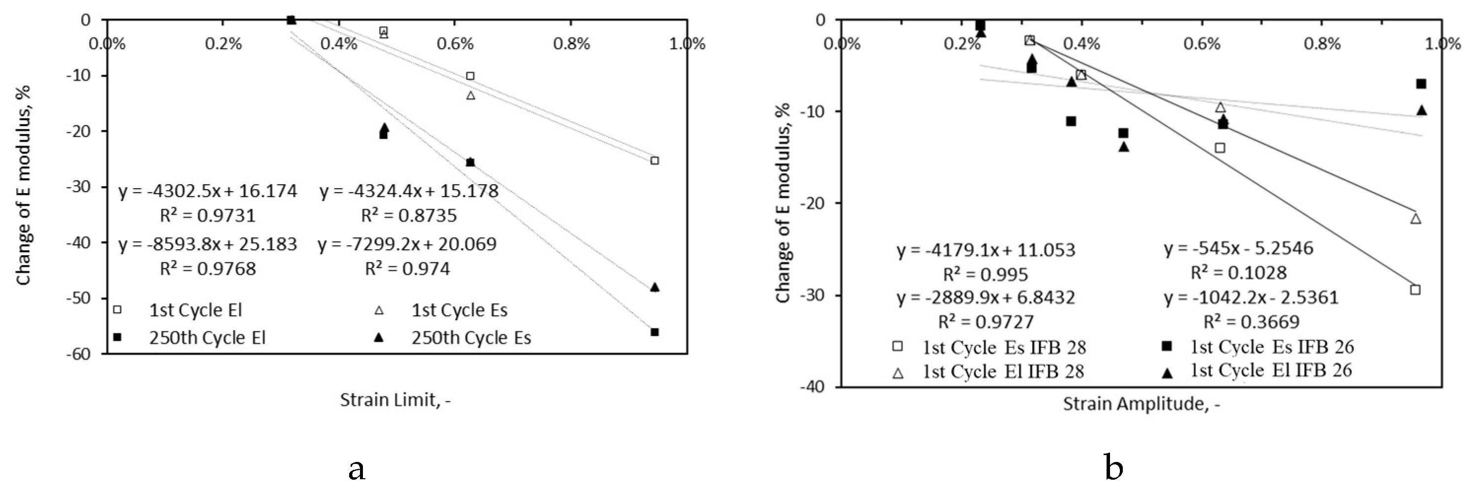
Figure 18.
Damage trends based on change of irreversible strain in cyclic tests of method II (a) and method III (b).
Figure 18.
Damage trends based on change of irreversible strain in cyclic tests of method II (a) and method III (b).
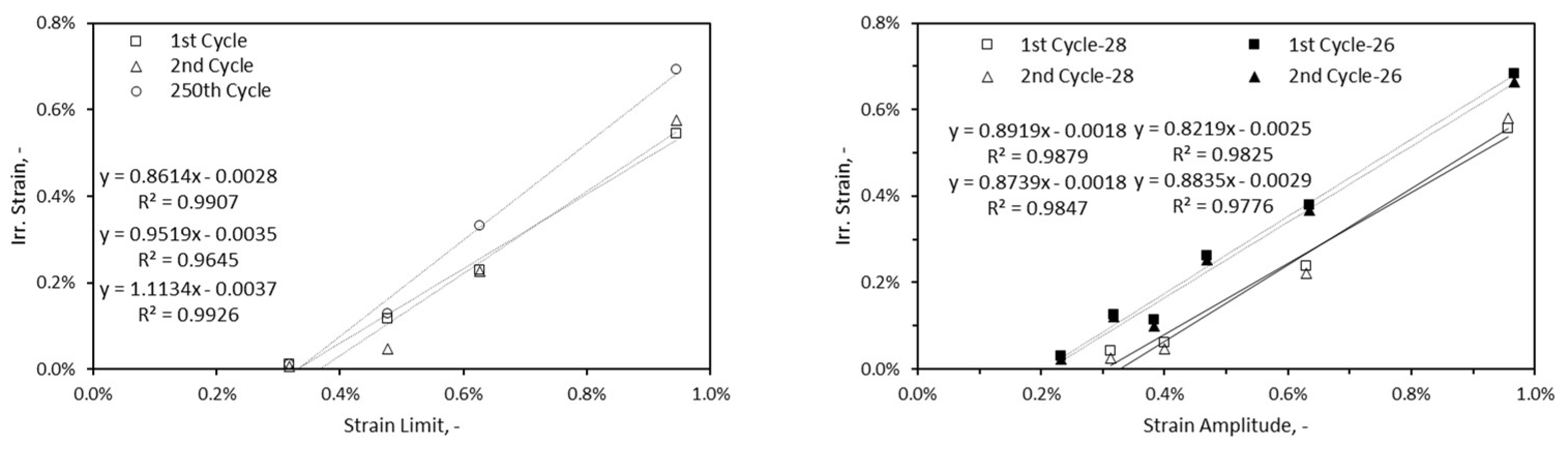
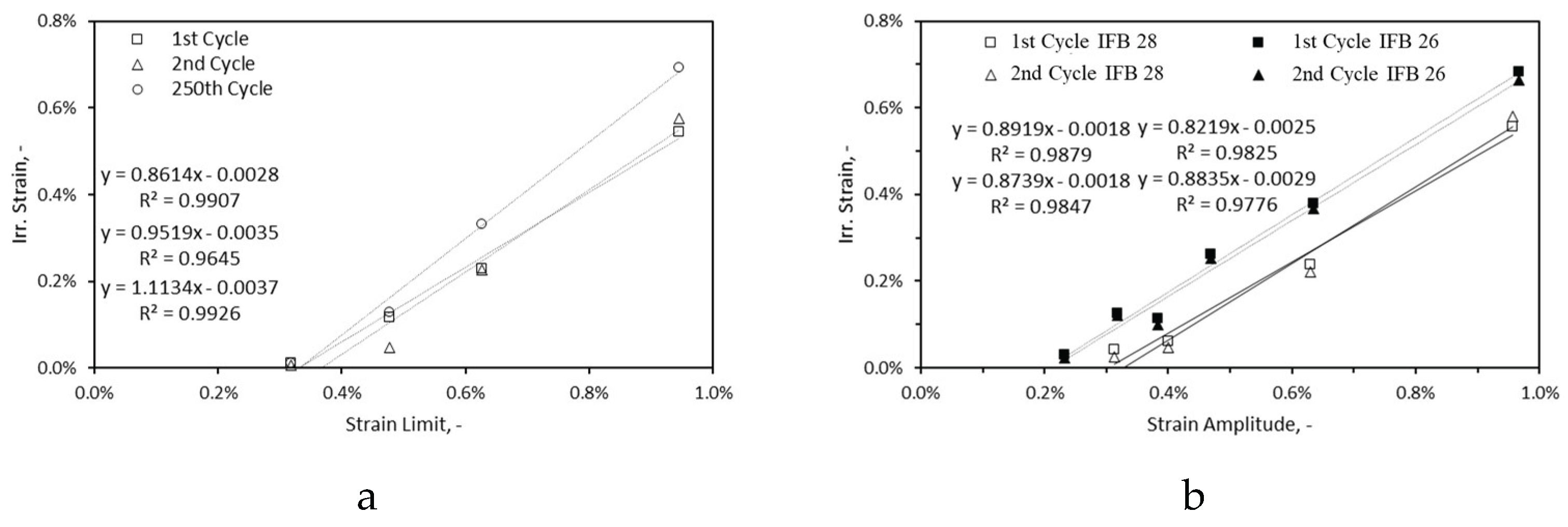
Figure 19.
Damage trends based on change of dissipated energy in cyclic tests of method II (a) and method III, IFB28(b) and IFB26(c).
Figure 19.
Damage trends based on change of dissipated energy in cyclic tests of method II (a) and method III, IFB28(b) and IFB26(c).
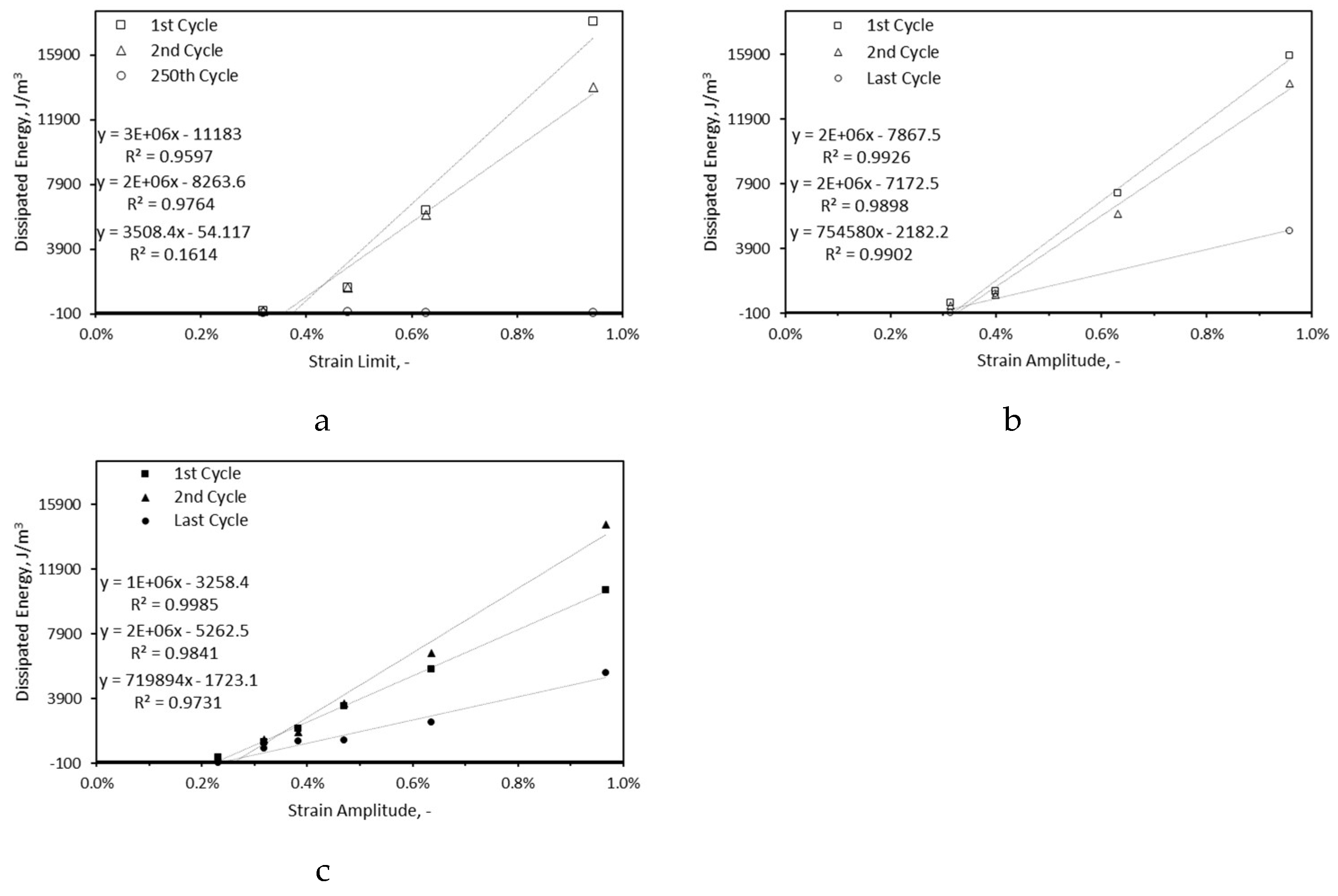
Figure 20.
Results of cyclic fatigue tests of method III. Arrows indicate samples with no failure.
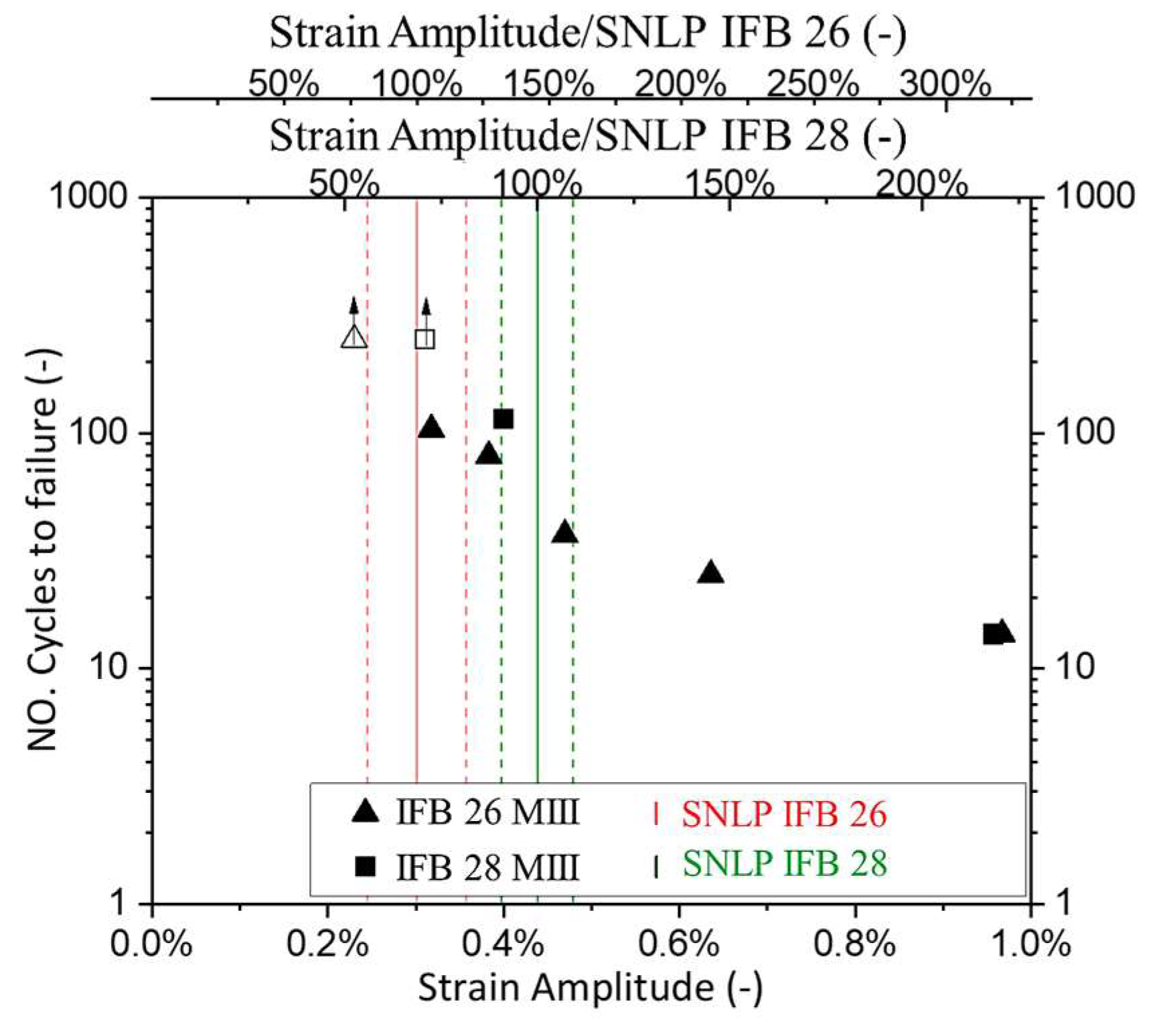

Table 1.
Materials’ properties.
| IFB 28 | IFB 26 | ||
| Chemical Composition | |||
| Al2O3 | [%] | 70.5 | 53.0 |
| SiO2 | [%] | 27.5 | 43.5 |
| K2O | [%] | <1 | <2 |
| Fe2O3 | [%] | <1 | <2 |
| Mineralogical Composition | |||
| Mullite 3:2 | [-] | Major | Major |
| Corundum | [-] | Major | Moderate |
| Quartz | [-] | Trace | Minor |
| Cristobalite | [-] | Trace | Trace |
| True Density | [g/cm3] | 3.26 | 2.95 |
| Bulk Density | [g/cm3] | 0.88 | 0.78 |
| Total Porosity | [%] | 72.6 ± 1.3% | 73.6 ± 1.4% |
Table 2.
Summary of the monotonic loading tests data. Mean values and coefficient of variation are shown.
Table 2.
Summary of the monotonic loading tests data. Mean values and coefficient of variation are shown.
| Property | IFB 28 | IFB 26 | |
|---|---|---|---|
| Compressive strength (CS) | [MPa] | 3.05 ± 5% | 2.34 ± 13% |
| Strain at maximal stress (SN) | [%] | 0.60 ± 28% | 1.30 ± 16% |
| Stress of linear proportion (SSLP) | [MPa] | 3.00 ± 6% | 1.88 ± 25% |
| Strain of linear proportion (SNLP) | [%] | 0.44 ± 9% | 0.30 ± 20% |
| SSLP / CS | [%] | 98.4 ± 6% | 80.5 ± 25% |
| SNLP / SN | [%] | 72.5 ± 9% | 23.1 ± 18% |
| Modulus of elasticity (ME) | [GPa] | 0.73 ± 9% | 0.62 ± 13% |
Disclaimer/Publisher’s Note: The statements, opinions and data contained in all publications are solely those of the individual author(s) and contributor(s) and not of MDPI and/or the editor(s). MDPI and/or the editor(s) disclaim responsibility for any injury to people or property resulting from any ideas, methods, instructions or products referred to in the content. |
© 2025 by the authors. Licensee MDPI, Basel, Switzerland. This article is an open access article distributed under the terms and conditions of the Creative Commons Attribution (CC BY) license (http://creativecommons.org/licenses/by/4.0/).
Copyright: This open access article is published under a Creative Commons CC BY 4.0 license, which permit the free download, distribution, and reuse, provided that the author and preprint are cited in any reuse.


