Submitted:
12 June 2025
Posted:
12 June 2025
You are already at the latest version
Abstract
Accurate real estate price estimation is a critical task in property markets, influencing both buyers and sellers. Traditional valuation methods often struggle to capture the complex, nonlinear relationships among property features and market trends. This thesis explores the application of machine learning models for predicting apartment prices using a dataset containing real estate listings from a city in Kyrgyzstan. Six models are evaluated: Linear Regression, Ridge, Lasso, Decision Tree, Random Forest, and Support Vector Machine. Two target variables are analyzed — total price and price per square meter — allowing for comparison of direct versus normalized pricing approaches.Model performance is assessed using multiple evaluation metrics, including Mean Absolute Error, Root Mean Squared Error, R-squared, and Mean Absolute Percentage Error. Random Forest consistently outperforms other models, achieving the highest predictive accuracy and generalization across both targets. The results demonstrate the effectiveness of ensemble learning in real estate valuation tasks and suggest practical implications for deploying ML models in automated property appraisal systems.
Keywords:
machine learning
; real estate
; valuation
; hypertuning
; regression
1. Introduction
1.1. Background and Motivation
Currently, real estate and construction are among the fastest growing sectors of the economy in many countries of the world. The need for accurate analytical tools to monitor a wide range of factors affecting the real estate market and dynamic fluctuations is increasing with the growth of the real estate market itself. For example, in Kyrgyzstan, the construction industry grew by 45% in the first half of 2024 alone (minstroy.gov.kg, 2025). In such an intense environment, digitalization of key business sectors can significantly optimize processes, increase resource management efficiency, and provide competitive advantages. One of these business processes is property valuation. This type of activity has always been and will always be the cornerstone for many other types of activities, including: making informed investment decisions, simplifying lending and insurance procedures, and optimizing taxation.
1.2. Problem Statement
Despite having large amounts of data, many valuation systems still use old-fashioned models or expert judgement. One of the most striking examples of this is the banks of the Kyrgyz Republic. Each bank should have a full staff of professional appraisers to evaluate collateral for lending or to evaluate mortgage loans. Often, the properties left as collateral in banks are the most standard apartments, houses, or cars, the valuation of which does not require special expert judgment. Banks often accept the most typical apartments, houses, and cars as collateral, which are evaluated based on average market indicators and do not require specialized expert opinion. However, such a practice can be vulnerable: firstly, it does not take into account the unique characteristics of a particular facility, and secondly, there is a risk of corruption - appraisers can be bribed to artificially inflate or underestimate the value, which leads to a distortion of financial risks and potential losses for credit institutions
Another open issue is taxation in the Kyrgyz Republic. At the moment, the property tax is calculated on the basis of zonal coefficients (salyk.kg, 2025), which are dictated by the state and may not always reflect real prices on the market. Having a completely independent algorithm for calculating the basic tax rate could significantly increase citizens' trust in tax institutions and strengthen the bond between citizens and the state.
1.3. Objectives
The core idea of this thesis is to explore different machine learning based approaches to auotomatically evaluate the price an apartment and analyze the importance of different factors that affect the market of apartments the most in the capital of the Kyrgyz Republic – Bishkek.
1.4. Scope and Limitations
The main problem in real estate valuation based on machine learning methods is the lack of data. Due to the weak digitalization of the country's regions, the development of such a system is currently expected only in the capital.
2. Literature Review
2.1. Traditional Approaches
Real estate valuation is the process of determining the market value of a property. In the practice of real estate valuation, three main traditional approaches are used: cost, sales comparison and income approach.
The cost approach is based on determining the value of real estate by calculating the costs necessary to reproduce or replace it, taking into account wear and obsolescence. This approach takes into account the cost of a land plot, the cost of building buildings and structures, as well as the cost of connecting to utility networks and other communications.
The sales comparison is based on an analysis of sales prices or offers of similar properties on the market. This approach involves comparing the assessed object with similar objects that have recently been sold or put up for sale. It is most effective in a developed real estate market, where there is a sufficient amount of information about transactions with similar properties (International Association of Assessing Officers, 2018).
The income approach is based on estimating the future profitability of a property and converting it to its current value. This approach is used to assess the investment attractiveness of real estate and determine its value based on expected income.
2.2. Machine Learning in Real Estate
Regression algorithms play a key role in estimating real estate prices because they allow you to predict continuous values, such as the cost of properties (Lee, 2025). Prior to this, attempts have been made several times to apply machine learning methods to evaluate real estate (The future of automated real estate valuations, 2022). For example, one such work is the startup Samai, which compared different models for evaluating houses based on data on purchases and sales in London from 1995 to 2019.
As a result, they obtained results that show that models based on traditional statistical methods are significantly inferior to machine learning methods. The authors of the article came to the same conclusions after analyzing the real estate market in Nizhny Novgorod . It is worth noting that in both works, the main characteristic that influenced pricing is location.
| Statistical Method Error | Machine learning method Error | |
| London (AAPE) 0.0016 -0.073 | 0.0016 | -0.073 |
| Nizhny Novgorod (MAPE) | 14.5 | 10.3 |
2.3. Challenges in Real Estate Price Prediction
One of the main problems in forecasting real estate prices is related to the specifics of the data itself. When training models on datasets from online ads, important time information is often missing. Ads reflect the state of the market at a certain point in time, but without explicit timestamps, it is difficult to account for seasonal trends, inflation, or market cycles.
As a result, models may not generalize well when applied to future data or in different market conditions, especially in rapidly changing urban environments.
An alternative to the data from the ads can be the official state registers of real estate transactions, which usually contain sales prices and dates. However, in countries such as Kyrgyzstan, the reliability of such data often suffers due to informal market practices.
Buyers and sellers often underestimate the value of transactions in official documents in order to reduce tax liabilities. This systematic underestimation leads to significant discrepancies between reported and actual market prices, making government data an unreliable basis for model training.
Thus, both data sources — online ads and official registries - have their significant limitations:
- Online data does not contain sufficient time information and may be distorted by seasonal fluctuations.
- Government data is often unreliable due to shady transactions and low prices.
Also listing prices often include negotiation margins or psychological pricing strategies, making them an imperfect proxy for actual willingness-to-pay. These factors significantly complicate the task of creating accurate and reliable forecasting models that require innovative approaches to processing and integrating various types of data to more accurately reflect the dynamics of the real estate market.
3. Methodology
3.1. Data Collection
Data for the analysis and training of models was collected from completely open sources, the main of which are house.kg and 2gis.kg in March 2025. Apartment listings, including details about price, location, number of rooms and other features,were parsed from the house.kg platform, whereas 2gis.kg was used to extract data about nearby facilities and infrastructure such as schools, hospitals, mosques. Also 2gis provides rating (by users) for each facility which is going to be fit as a feature.
3.2. Data Preprocessing
After the data was collected, it went thorough preprocessing to ensure consistency and compatibility with machine learning models:
- Translation: All feature names and categorical values were translated from Russian to English to maintain uniformity.
- Outlier Detection and Removal: Listings with extreme or implausible values (e.g., unusually high prices) were identified and excluded.
- Data Imputation: Missing values in both numerical and categorical fields were handled using appropriate imputation strategies, such as mean substitution or assigning default category labels.
- Encoding Categorical Features: Categorical variables, such as building type and district, were encoded using either label encoding or one-hot encoding, depending on the model requirements.
- Normalization of Numerical Features: Numerical features like price, area, and number of rooms were normalized to improve convergence in models that are sensitive to feature scaling.
It is worth mentioning that some preprocessing procedures—particularly encoding and normalization—were adjusted to comply with the specific requirements of different machine learning models. For instance, most of the gradient boosting algorithms (e.g., XGBoost, LightGBM) don't require normalization of categorical features and may even natively support categorical data.
3.3. Modeling Approaches
3.3.1. Linear Regression
Linear Regression is considered to be the easisiest and the most well-statied method for the problems of regression (James, Witten, Hastie, & Tibshirani, 2013). In general, linear models have the following form (Linear models, 2025):
- To evaluate how well the model’s predictions align with the true values, we define a loss function. One commonly used function is the Mean Squared Error (Linear models, 2025):
Now, methods of optimization may be applied to minimize the value of the loss. The most popular algorithm for optimizing machine learning models is called Gradient Descent (Vasques, 2024). It iteratively updates the values of the weight vector, until a convergence at which local minima is reached:
One of the most important terms in this formula is – learning rate. This hyperparameter used to control how fast that convergance is going to be reached. Too large value for may lead us to the situation when we skip local minima. That’s why usually the value for is chosen after multiple experiments, manually changing it for each one, altough nowadays we have more advanced methods to adjust hyperparameters (Akiba, Sano, Yanase, Ohta, & Koyama, 2019).
In our case, for real esate price evaluation, linear regression model becomes:
3.3.2. Ridge/Lasso Regression
Linear regression as its pure form is prone to overfitting. This phenomenon occurs when our features are highly correlated with each other and model becomes too complicated with large weights. It may lead to the situation when model predicts well on the training data and shows poor result on the data that it hasn’t seen so far. This property of models to perform well on new, unseen data is referred to as generalization.
Two widely used techniques to introduce generalization in Linear Regression models are Lasso Regression (L1 Regularization) and Ridge Regression (L2 Regularization) (James, Witten, Hastie, & Tibshirani, 2013).
They have forms
3.3.3. Random Forest
Random ForestRandom Forest is an ensemble learning method that constructs multiple decision treesduring training and aggregates their predictions to improve accuracy and stability (?).For regression tasks, such as predicting apartment prices, it outputs the mean predictionacross all trees. Each tree is trained on a random subset of the dataset (via bootstrap-ping) and a random subset of features at each split, reducing overfitting and enhancinggeneralization. The final prediction for an input x is given by:
where is the predicted value, T is the number of trees, and is the prediction of the t-th tree.
3.3.4. Support Vector Machine (SVM)
Support Vector Machine is a powerful supervised learning algorithm that can be used for both classification and regression tasks. For regression problems, known as Support Vector Regression (SVR), SVM aims to find a function that deviates from the actual target values by no more than ε (epsilon) while being as flat as possible (Vapnik & Cortes, 1995).
3.4. Evaluation Metrics
3.4.1. Coefficient of Determination (R2)
The R² metric measures the proportion of variance in the target variable that can be explained by the input features. It is defined as:
where is the actual value, is the predicted value, is the mean of actual values, is the number of observations. An value close to 1 indicates a high proportion of explained vairance, while a value near 0 implies poor explanatory power. In the context of real estate, a higher signifies that the model captures the target value well.
3.4.2. Mean Absolute Percentage Error (MAPE)
MAPE measures the average magnitude of prediction errors as a percentage of actual values. It is especially intuitive for stakeholders in the real estate industry, as it conveys how far off, on average, the predictions are from actual prices:
MAPE is scale-independent and interpretable; for example, a MAPE of 10% means that predictions are off by 10% on average. However, it is sensitive to small denominators and may be skewed when values are close to zero.
4. Exploratory Data Analysis
4.1. Overview of the Dataset
The dataset used in this study consists of overall ~7400 apartments with 11 features. The price of of an apartment in USD is set to be primary target variable.

Table 1.
Dataset Description.
| Feature | Type | Description |
|---|---|---|
| Area | Number | Total area of an apartment given in m2 |
| Series | Category | Apartment series1 |
| Floors | Number | The floor where the apartment is located |
| Floors number | Number | Total number of floors in the building |
| Rooms number | Number | Total number of rooms in the apartment |
| Construction Year | Number | Year when apartment was constructed |
| Heating | Category | Heating type (“Gas”, “Electric” etc) |
| Condition | Category | Technical condition of the house |
| Wall material | Category | Wall material (“Brick”, “Panel” etc) |
| Latitude | Number | |
| Longitude | Number |
Table 2.
Dataset statistics.
| Mean | Std Dev | Min | Max | |
|---|---|---|---|---|
| Area (sqm) | 76.6 | 43.1 | 10 | 650 |
| Floor | 6.6 | 3.9 | 1 | 21 |
| Number of Floors | 10.8 | 3.9 | 1 | 25 |
| Number of Rooms | 2.2 | 0.99 | 1 | 6 |
| Built Year | 2017.6 | 13 | 1952 | 2028 |
| Price ($) | 110,707 | 75059 | 19,000 | 1,500,000 |
| Price per sqm ($) | 1430 | 345.8 | 305 | 3440 |
4.2. Distribution of the Target Variables
As shown in the Figure 1, first target variable (overall Price) has right-skewed distribution. This skewness is essential for real estate data because of the presence of a small number of luxury apartments costing significantly above the mean. But overall, most of the apartments lie in the range from 50,000$ to 150,000$.
But if we look at the distribution of the second target variable in Figure 2. Distribution of Price per Square meter, which is Price per sqm, it has almost perfect normal distribution that is more suitable for fitting to machine learning models, even though it also does have some little right-skewness. The average price per meter square lies in the range of from $1000 to $1600.
4.3. Correlation Analysis
The goal of this section is to examine the relationships between the numerical features in the dataset and identify those that are most strongly related to the target variables.
Pearson correlation coefficients have been computed between all pairs of numerical features and target variables. The pearson correlation coefficient measures linear independence:
- : perfect positive linear correlation
- : perfect negative linear correlation
- : no linear correlation
- As it can be seen in Figure 4, Area has the strongest correlation with the total price, which is expected. We also observe that we have very few features that negatively correlate with both of our target variables, only derived features like Number of hospitals withing 1 km are showing a coefficient with the values at most -0.2.
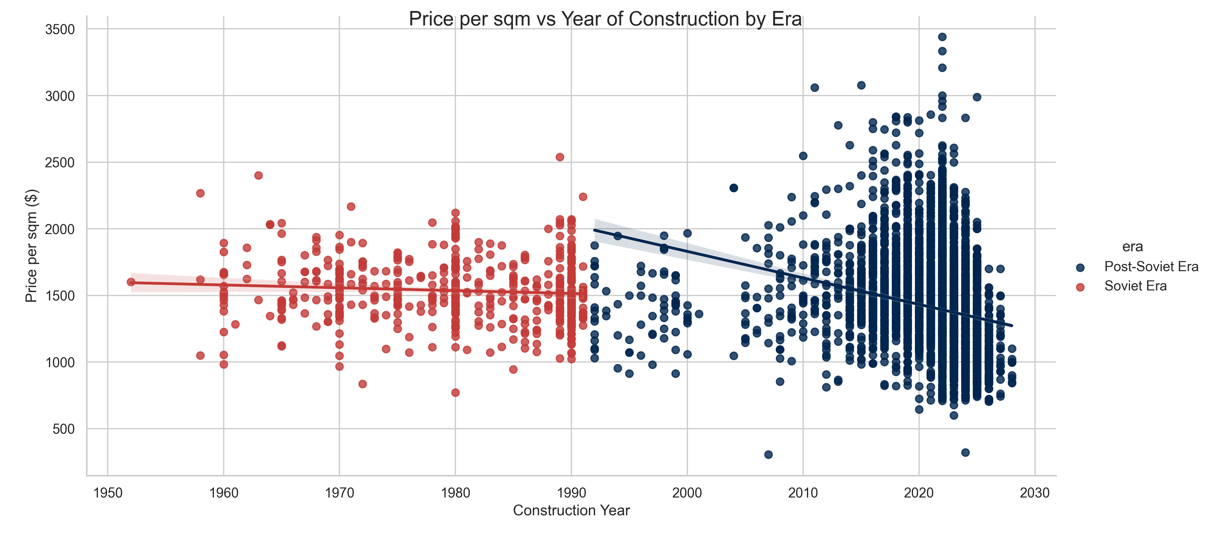
- Also we can employ scatterplot to gain more useful insights about the correlation of some specific features. For exampe, in the Figure 4 it is clearly seen that construction year has positive correlation with the price. The chart also suggests that the collapse of Soviet Union has introduced the market more diversification in terms of price and area.
5. Implementation
5.1. Model Training & Evaluation
5.1.1. Metrics
5.1.2. Linear Regression (Baseline)
A standard Linear Regression model was trained on the dataset as a baseline for other models. The model was fit using sklearn.linear_model.LinearRegression without any regulatization techniques. It is worth noting that sklearn fits this model analytically (Liu, 2018), and does not perform any training process, hence there is no need in hypertuning.
5.1.3. Ridge & Lasso
These models are the same as a simple Linear Regression but with regularization included. Both models require one additional hyperparameter – regularization strength, even though they are also fit analitically.
5.1.4. Decision Tree
A decision tree models was also trained using sklearn.DecisionTreeRegressor. Key hyperparameters in this model were tuned using Optuna.
6. Results
6.1. Model Performance
Among all the tested models, Random Forest demonstrated superior performance in both target variables — total price and price per square meter — achieving the lowest values of MAE, RMSE and MAPE and the highest values of R2 (Table 3. Metrics). This suggests that complex methods are particularly well suited for real estate price forecasting tasks. On the contrary, linear models, despite their interpretability, have proved ineffective due to their limited ability to model the nonlinear relationships inherent in housing stock data. The results also show that forecasting the price per square meter yields a slightly lower percentage of errors, although this may be due to difficulties in interpretation or practical application.Feature importnace analysis.
6.2. Residual Analysis
The graph "Residuals vs Fitted" shows pronounced heteroscedasticity: the variance of errors increases significantly with an increase in the forecasted value of real estate. This suggests that the model does not capture the factors influencing the price well, especially in the segment of expensive real estate.The Q-Q graph (Figure 5. Plots of the residuals) confirms the abnormality of residuals with heavy tails, which indicates frequent extreme forecasting errors. This violates the assumptions underlying standard inference methods and can make it difficult to obtain reliable confidence intervals. The histogram of the residuals shows a strong right-hand bias and bimodality, which implies the presence of various error modes and possibly reflects unaccounted-for differences between the luxury and standard real estate markets.Finally, the "Actual versus Predicted Values" graph reveals a systematic bias: mid-range real estate is overestimated, while luxury real estate is underestimated.Taken together, these diagnostic data emphasize the need for either nonlinear feature processing (for example, polynomial location effects), stratified modeling by price category, or transformation of the target variable (for example, using the logarithm of price) to reduce heteroscedasticity and improve forecasting accuracy in the segment of expensive real estate.
7. Conclusions
This study examined the use of machine learning models to estimate real estate prices in Bishkek, Kyrgyzstan. This is especially important for fast-growing markets where accurate and automated assessment systems are needed. Using a dataset of approximately 7,400 apartment rows, six regression models were evaluated: linear regression, ridge, lasso, decision tree, random forest, and support vector machine. The models were evaluated based on two target variables: the total price and the price per square meter.
Key finding – the superiority of ensemble methods: the Random Forest model proved to be the most effective, achieving the highest prediction accuracy (R2 = 89.55% for the total price and 87.87% for the price per square meter) and the lowest errors (MAE: 8,883 dollars; MAPE: 10.32%). Its ability to account for non-linear feature interactions and outlier tolerance highlights its suitability for heterogeneous real estate markets.
The study demonstrates that machine learning, especially the Random Forest method, offers a robust framework for evaluating real estate in Kyrgyzstan. By combining traditional valuation techniques with modern data science, this work lays the foundation for fair and efficient real estate markets.
References
- Akiba, T., Sano, S., Yanase, T., Ohta, T., & Koyama, M. (2019). Optuna: A Next-generation Hyperparameter Optimization Framework. 25th ACM SIGKDD International Conference on Knowledge Discovery and Data Mining, (pp. 2623–2631). Anchorage. [CrossRef]
- International Association of Assessing Officers. (2018). Retrieved from “Standard on Automated Valuation Models (AVMs) International Association of Assessing Officers: https://www.iaao.org/.
- James, G., Witten, D., Hastie, T., & Tibshirani, R. (2013). An Introduction to Statistical Learning with Applications in R. New York: Springer.
- Lee, S. (2025, March 27). How Machine Learning Enhances Property Value and Investment. Retrieved from Number Analytics: https://www.numberanalytics.com/blog/machine-learning-enhances-property-value-investment.
- Linear models. (2025, May 7). Retrieved from education.yandex.ru: https://education.yandex.ru/handbook/ml/article/linear-models.
- Liu, Y. (2018, 11 1). Analytical Solution of Linear Regression. Retrieved from medium.com: https://medium.com/data-science/analytical-solution-of-linear-regression-a0e870b038d5.
- (n.d.). Massovaya ocenka ob"ektov nedvizhimosti na osnove tekhnologij mashinnogo obucheniya. Analiz tochnosti razlichnyh metodov na primere opredeleniya rynochnoj stoimosti kvartir.
- minstroy.gov.kg. (2025, May 7). Retrieved from minstroy.gov.kg: https://minstroy.gov.kg/ru/news/430/show.
- salyk.kg. (2025, May 7). Retrieved from calculator.salyk.kg: https://calculator.salyk.kg/infosti086.
- (2022). The future of automated real estate valuations. Saïd Business School.
- Vapnik, V., & Cortes, C. (1995). Support-vector networks. Machine Learning, 273-297.
- Vasques, X. (2024). Machine Learning Theory and Applications. Bois-Colombes: Wiley.
| 1 | Apartments built during the Soviet era typically follow specific standardized series (building types), which can influence their layout, construction quality, and market value. Check: https://www.salut.kg/serii.php
|
Figure 1.
Distribution of Price.
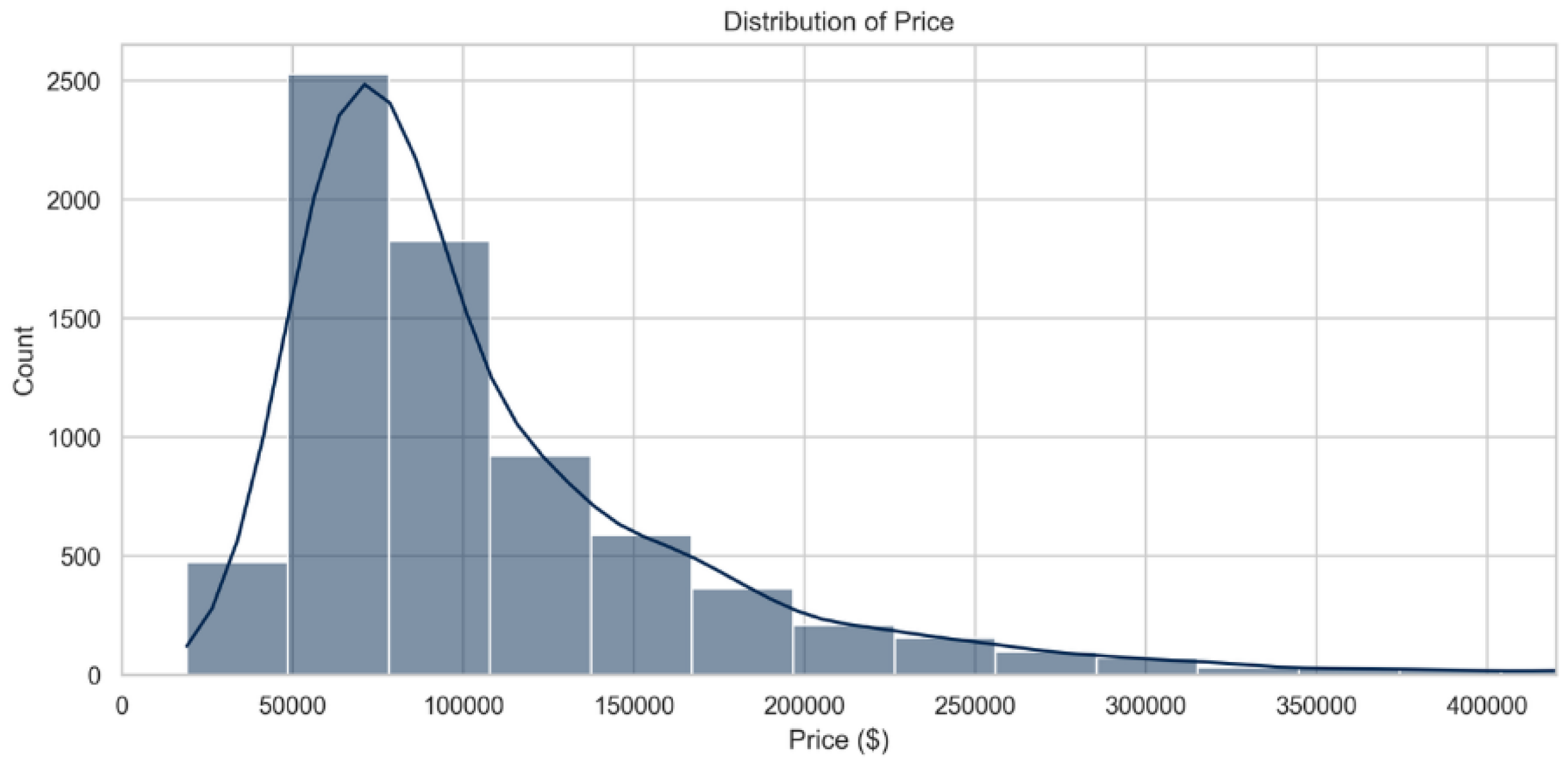
Figure 2.
Distribution of Price per Square meter.
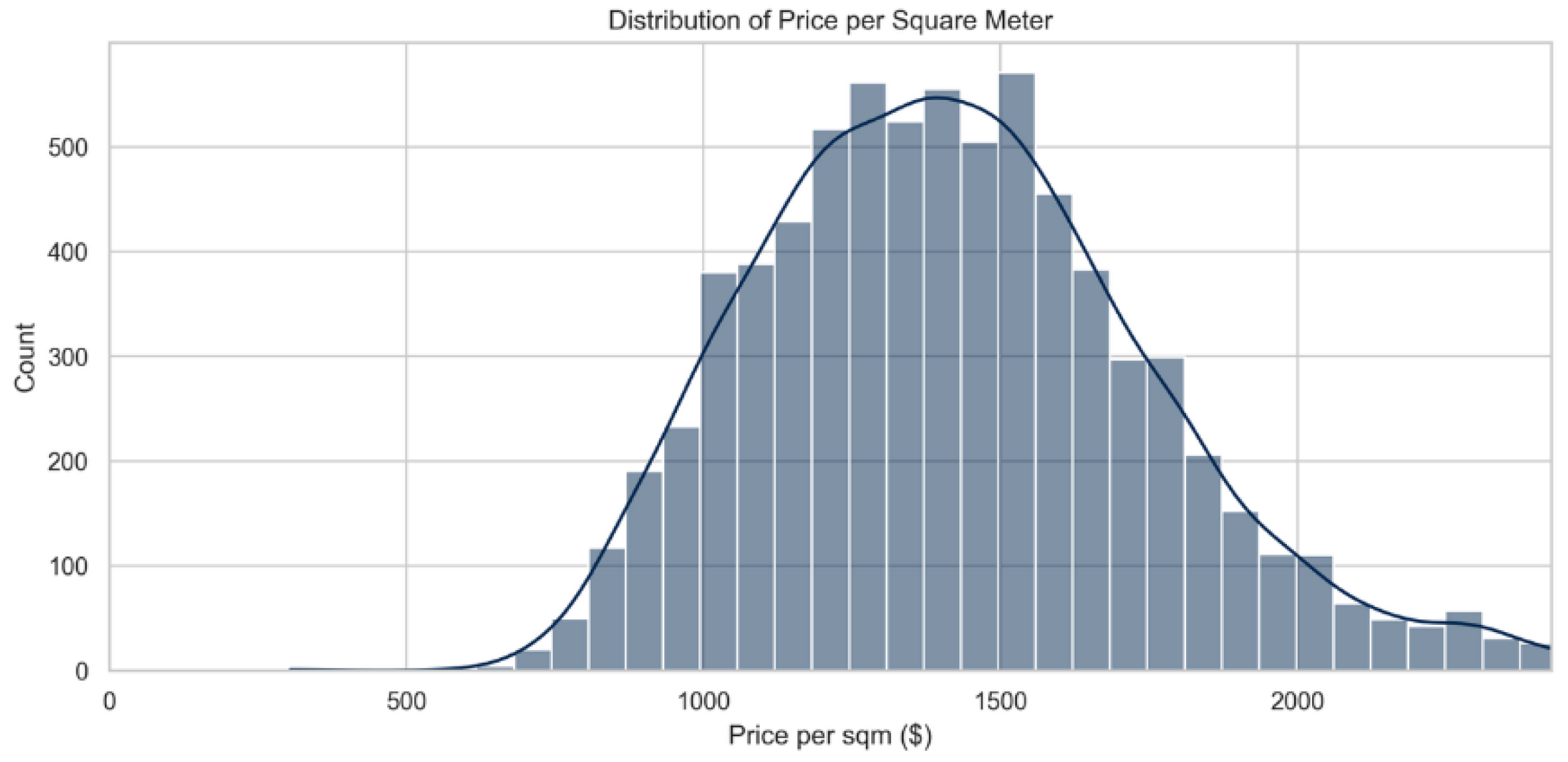
Figure 3.
Pearson Correlation of Numerical Features with Target Variables.

Figure 4.
Price vs Year of construction.
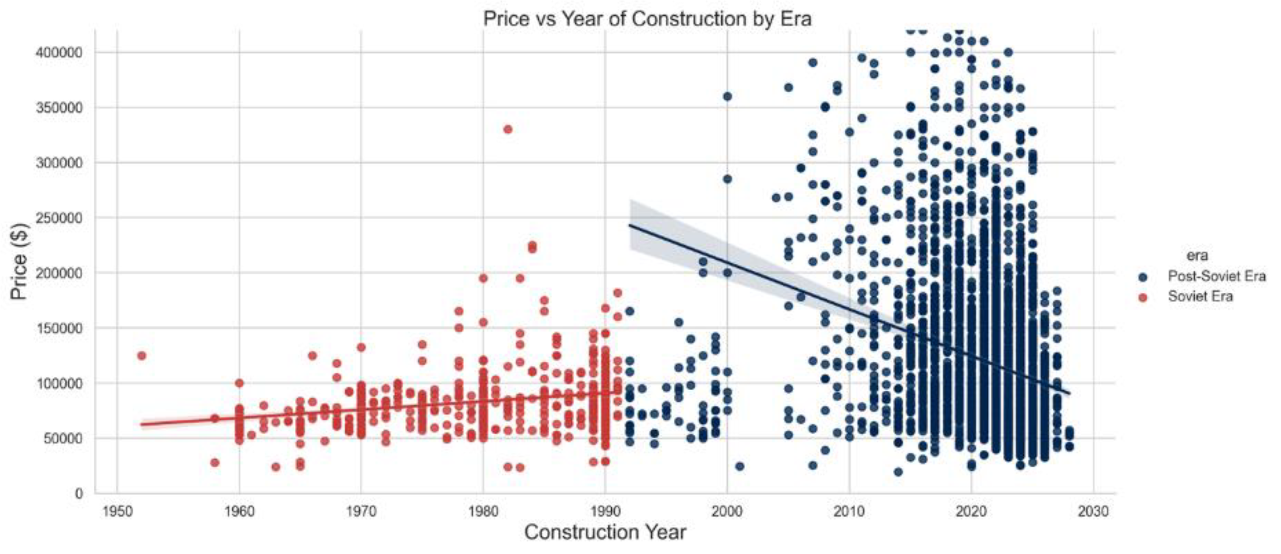
Figure 5.
Plots of the residuals.
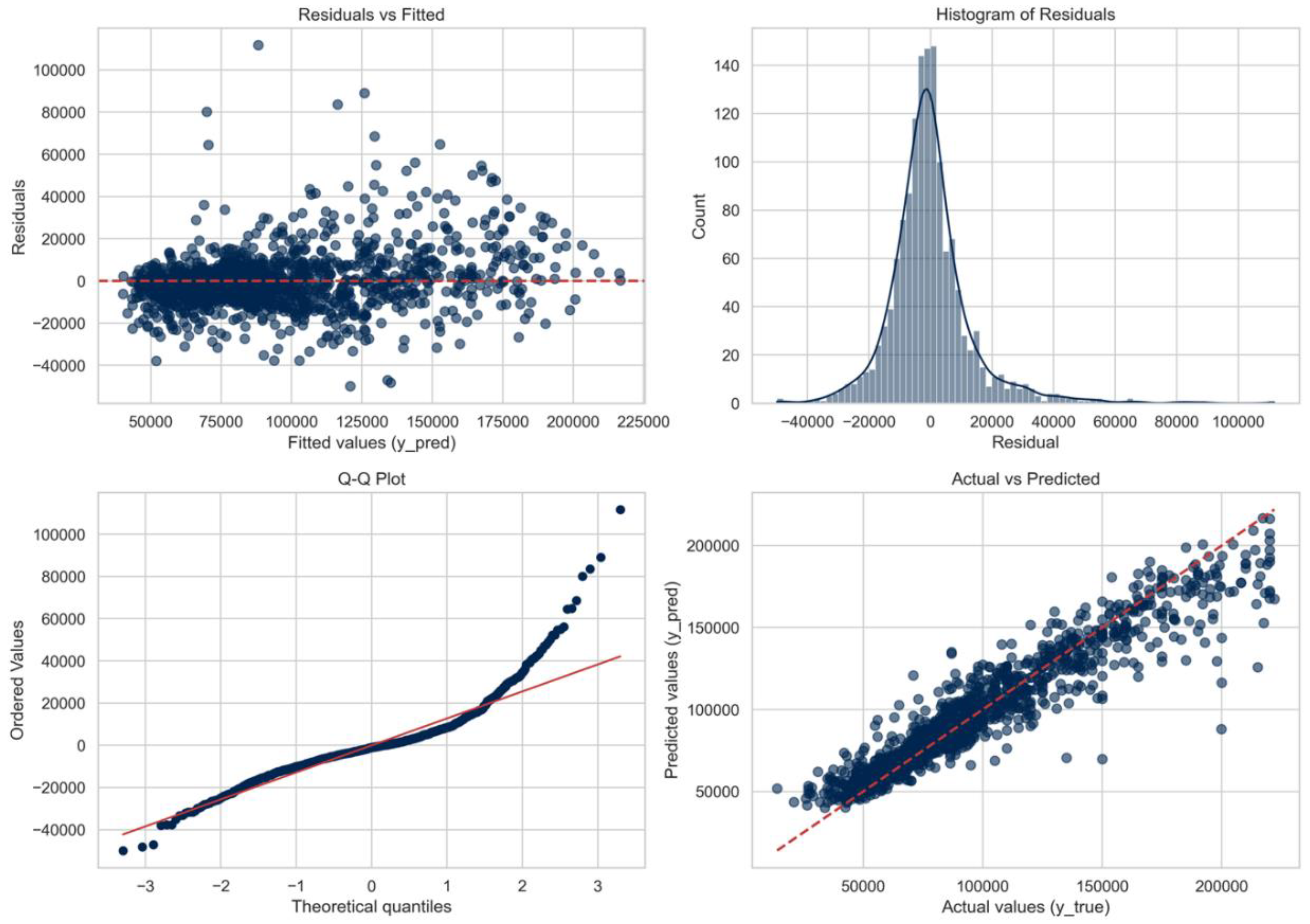
Table 3.
Metrics.
| MAE | RMSE | R2 (%) | MAPE (%) | |||||
|---|---|---|---|---|---|---|---|---|
| 1 | 2 | 1 | 2 | 1 | 2 | 1 | 2 | |
| LR | 13,458 | 12,737z | 19,007 | 18,565 | 78.19 | 79.31 | 15.16 | 13.56 |
| LR (Ridge) | 13,455 | 12,737 | 19,006 | 18,566 | 78.19 | 79.31 | 15.16 | 13.67 |
| LR (Lasso) | 13,511 | 12,813 | 19,014 | 18.663 | 78.18 | 79.09 | 15.24 | 13.68 |
| Decision Tree | 10,766 | 10,64 | 16,374 | 17,305 | 83.82 | 82.03 | 11.73 | 10.68 |
| Random Forest | 8,883 | 8,367 | 13,154 | 14,219 | 89.55 | 87.87 | 10.32 | 9.02 |
| SVM | 12,937 | 12,727 | 19,065 | 18,933 | 78.06 | 78.49 | 14 | 13.24 |
Disclaimer/Publisher’s Note: The statements, opinions and data contained in all publications are solely those of the individual author(s) and contributor(s) and not of MDPI and/or the editor(s). MDPI and/or the editor(s) disclaim responsibility for any injury to people or property resulting from any ideas, methods, instructions or products referred to in the content. |
© 2025 by the authors. Licensee MDPI, Basel, Switzerland. This article is an open access article distributed under the terms and conditions of the Creative Commons Attribution (CC BY) license (http://creativecommons.org/licenses/by/4.0/).
Copyright: This open access article is published under a Creative Commons CC BY 4.0 license, which permit the free download, distribution, and reuse, provided that the author and preprint are cited in any reuse.


