Submitted:
12 June 2025
Posted:
12 June 2025
You are already at the latest version
Abstract
Total Electron Content (TEC) allows to evaluate the state of the ionosphere. Radio waves like GNSS signals traversing the ionosphere suffer delays and refraction. Ionospheric plasma irregularities may be generated in the equatorial regions after sunset and extend to low latitudes forming large plasma depleted regions named ionospheric bubbles. Signature of these bubbles can be observed at TEC maps. Inside plasma bubbles smaller scale size irregularities are generated causing scintillation in GNSS signals. This work compared TEC maps from some sources, with different temporal and spatial resolutions/coverage. Significant differences were found. For each source, there are differences in the treatment and preprocessing of raw data in order to get the absolute TEC values, which are interpolated to get grid values of the map. Even for the same source there are significant differences in the density of monitoring stations according to the region. A case of study concerning scintillation is also analyzed using the corresponding TEC and scintillation maps. TEC maps employed here encompass the years from 2022 to 2024, in the growing phase of the current solar cycle 25. The months of March, June, September and December were selected to take into account the TEC seasonal variation.
Keywords:
total electron content
; TEC maps
; TEC measurements
; ionospheric irregularities
1. Introduction
The Total Electron Content (TEC) field allows to evaluate and model the state of the ionosphere, which is affected by the space weather. This work compares bidimensional TEC maps from different sources.
Space weather is related to Earth interaction with outer space, being the biggest effect due to the Sun. Solar activity influences Earth magnetic and electric fields, which influence the ionosphere, a layer of the atmosphere that ranges from 50 to 1,000 km of altitude composed of plasma, i.e. ions and free electrons. Plasma density varies with altitude since it depends on the intensity of the solar ionizing radiation, plasma absorption by atmospheric gases through ion recombination and electron-capture processes, ion recombination, and electron-capture processes. Dynamic processes like diffusion, plasma drifts and neutral winds also affect the plasma density profile. In the ionosphere there is a competition between ionization production due to the Sun radiation and ionization losses due to the recombination of ions and electrons. The ionospheric ionization is much larger during sunlight hours than nighttime hours when there is no more solar radiation. The ionosphere also is influenced by seasonality, geographic location, phase of the solar cycle, and magnetic storms [1].
Radio frequency signals between satellites and ground receivers are affected by the ionosphere, mainly by perturbations known as ionospheric scintillation, caused by irregularities of the ionospheric density. The most important of these radio signals are from Global Navigation Satellite Systems (GNSS), constellations of satellites that provide precise geographic position to receivers in aircrafts, ships, vehicles and ground stations. Once the GNSS receiver acquires a lock with at least four satellites, its position is calculated by triangulation from each estimated receiver-satellite distance. Currently operational GNSS are the American Global Positioning System (GPS), the Russian Global Navigation Satellite System (GLONASS), the Chinese BeiDou Navigation Satellite System (BDS), the European Galileo, and the Japanese Quasi-Zenith Satellite System (QZSS) [2].
The TEC field is estimated from dual-frequency measurements of phase delay, or adding the pseudorange, made by receivers of networks of ground stations. Worldwide or regional TEC maps are obtained by interpolating local TEC values derived from measurements acquired by these receivers. Mathematical models are also used to generate the TEC field and the corresponding maps, but usually are not accurate due to low temporal or spatial resolutions, and lack of assimilation of data from GNSS stations.
During daylight the equatorial ionospheric plasma is lifted up due to eastward electric fields. After sunset and until about 21 LT (local time) this upward plasma movement is intensified, giving origin to a large vertical electron density gradient at the ionospheric F region base, which is one condition for plasma irregularities to be generated through the Rayleigh Taylor mechanism [3].
One ionospheric anomaly is the Equatorial Ionization Anomaly (EIA), which occurs about 15° magnetic degrees north and south of the dip equator, characterized by larger background electronic density during the pre-reversal hours (18-21 LT) compared to lower latitudes [4]. The TEC field at EIA shows crests with high gradients, which are associated with the eventual occurrence of strong scintillation.
The most common of the ionospheric irregularities are the ionospheric bubbles, low-density structures (low TEC values) that are formed near the magnetic equator or at low magnetic latitudes, mostly in the equinoxes and summer of years of high solar maximum activity. These bubbles are created 1-to-2 hours after sunset, expand along the magnetic north and south directions, then migrate to the magnetic south and west directions, and disappear before midnight and sometimes 1-to-2 hours after midnight. Inside the equatorial plasma bubbles, small-scale ionospheric plasma irregularities are generated, causing amplitude and phase scintillation which affects RF communication in the L band, for instance GNSS navigation. Ionospheric scintillation is measured by the amplitude and phase indexes. Amplitude scintillation is given by the S4 index, calculated as the normalized standard deviation of the GNSS signal intensity for 1 minute with a sampling rate of 50 Hz [5]. Phase scintillation is given by the σφ index, calculated as the standard deviation of the detrended phase in each 1-minute interval [5,6]. Scintillation typically occurs in the months of September to March in Brazil.
Besides the increased frequency of bubbles in the equinoxes and summer, there is a high variability throughout the year, making it difficult to predict their occurrence. TEC gradients in a bubble can reach 30-50 TEC units (TECU) for some hundreds of kilometers [7,8]. Similarly to scintillation, these bubbles occur in general between the months of September and March in Brazil, presenting high TEC gradients and affect the ionosphere refraction index. They may cause scintillation, disturbing GNSS and telecommunication signals in amplitude and phase [9].
Time series of TEC maps are intended to identify the formation and the evolution of ionospheric bubbles over time. There are many methodologies [7,8,10,11,12,13,14,15,16,17] being employed by scientific institutes or governmental organizations for the continuous monitoring of the ionosphere by means of TEC maps. This work aims to compare TEC maps of different sources, trying to suggest which one is more suitable for ionosphere monitoring over Brazil and to present examples of bubble signatures observed at TEC maps.
TEC maps employed here encompass the years from 2022 to 2024, in the current solar cycle growing phase. Some months were chosen each year, March, June, September and December to represent seasonal behavior. One of the former reasons for this study was to choose a suitable source of TEC maps over Brazil in order to perform predictions of TEC maps from time series of TEC maps using neural networks. There is an abundance of works using TEC maps, but from different sources. Because of the variety of institutions that generate TEC maps with differing methods, resolutions, and GNSS sources, understanding how consistent and accurate such products are, especially over low-latitude regions like Brazil, is important.
This article aims to provide a systematic comparison of TEC maps from four major sources across the Brazilian region by statistical correlation analysis and scintillation indices and regional TEC measurements validation. The results are intended to support suitable TEC data sets accordingly for scientific and application use. This comparative relative basis is particularly significant in regions where ionospheric irregularities, such as equatorial plasma bubbles, are prevalent and could drastically degrade signal quality [18,19]. Despite numerous TEC map products, few research works have performed a comprehensive comparative investigation over South America using homogeneous spatiotemporal standards and ground truth validation.
This work checked TEC maps from 4 of these sources, according to their temporal and spatial availability, considering coverage of the Brazilian territory, and found significant differences. Each source corresponds to a given institute or organization, and obviously, there are differences in the treatment and preprocessing of raw data provided by GNSS stations in order to get the absolute TEC values in each point of the map.
The proposed comparison required a search for temporal and spatial gaps of the time series of maps of each source, which are due to lack of data, thus filtering the available maps. Each map is considered as the matrix that contains its latitude x longitude point TEC values, referred as TEC map data. Even for the same source there are significant differences in the density of monitoring stations around the globe. Each TEC data source can be realized as a kind of reference that allows the development of scientific studies specifically based on it. A filtering concerning available time periods was done in order to assure overlapping periods, followed by an interpolation performed to obtain a unified spatial resolution. TEC map data from different sources over Brazil are then compared by means of Pearson correlation values between each pair of maps and between each pair of sources.
These maps are also compared with TEC point measurements of a specific GNSS station located at São José das Campos, Brazil, since point measurements are expected to be more accurate than TEC values extracted from TEC maps. The proposed comparison is intended to choose the best TEC map over Brazil, if any. As already mentioned, better TEC maps allow a suitable monitoring of Earth’s ionosphere, identifying irregularities such as ionospheric bubbles. Good spatial and temporal resolution are then required.
2. Materials and Methods
2.1. TEC Maps Sources
The ionosphere can be modeled by the TEC field, depicted by latitude-longitude maps. Values of TEC in these maps are obtained assuming the ionosphere as a thin layer at a defined altitude. TEC is the electron density (ne) given by the line integral along the signal slant path s from receiver to satellite, considering a column of one-meter-square cross section centered on the path, which is given in TEC units, defined as 1 TECU = 10¹6 electrons/m² (Equation 1).
Typical TEC values measured near the Earth’s surface range from about 1 to 150 TECU [20] with the actual value depending on geographic location, local time, season, solar flux, and magnetic activity. The relative slant TEC (STEC) can be characterized by observing carrier phase delays of the received RF signal transmitted from GNSS satellites. The carrier phase and pseudorange observables recorded by a multi-frequency GNSS receiver allows to estimate the STEC. Equation 2 presents the STEC calculation using the GNSS signal phase (there is another equation using the pseudorange, not shown in this work):
In the above Equation, f1 and f2 are the two carrier frequencies of the GNSS signals, L1 and L2 are the carrier phase counts, and K ≈ 40.3 m3 s−2.
Better TEC maps are derived using higher temporal and spatial resolutions, but global maps may have accuracy compromised by TEC data provided by low density of TEC monitoring stations according to the region. In the case of TEC map prediction, a long time series may be required, and the extension of the time series varies widely for different sources. TEC map prediction using machine learning requires a long time series in order to perform the training of a neural network (most common case). Another point is to have a time series covering entire solar cycles, not only solar maximum or solar minimum. However, this study covers the current growing phase of the solar cycle 25. Two global and two regional TEC map sources are analyzed here. Table 1 describes these four TEC map sources.
2.1.1. IGS (International GNSS Service)
The International GNSS Service (IGS) was established in 1998 with the objective of generating reliable global vertical Total Electron Content (VTEC) maps [21]. It supplies combined Global Ionospheric Maps (GIM), which are obtained as a simple weighted mean of the VTEC maps produced by the available Ionospheric Associate Analysis Centers (IAAC) (https://igs.org/products/#ionosphere), also called IGS Working Groups. There are currently 7 of these groups: Center for Orbit Determination in Europe (CODE), European Space Agency (ESA), National Aeronautics Space Administration (NASA) Jet Propulsion Laboratory (JPL), Universitat Politècnica de Catalunya (UPC), Natural Resources Canada (NRCan), Chinese Academy of Sciences (CAS) and Wuhan University (WHU). The latter three started contributions in 2016, and the remaining, since 1998. These GIMs have been combined since 2007 by the University of Warmia-Mazury (UWM) to generate the IGS combined GIM [14].
The IGS VTEC combined maps in the IONosphere map Exchange (IONEX) format include a “final solution” product with ~11 days latency and weekly updates, and a “rapid solution” product with less than 24-hour latency and daily updates. The reliability and accuracy of the combined IGS GIM primarily depend on the fair evaluation of the consistency and accuracy of individual GIMs, provided by the different centers [11,13].
Further information about these maps is detailed below:
- Product: IGS combined GIM (VTEC maps);
- Temporal coverage: since 2/6/1998 (according to data repository);
- Latency: “final solution” with ~11 days; “rapid solution” with less than 24 hours [11];
- Single layer shell height: 450 km (according to IONEX data information);
- GNSS constellations: GPS and GLONASS [11];
- GNSS stations: IGS (international) (https://igs.org/faq/#igs-network-stations);
- Data format: IONEX [22];
- Data repository: https://cddis.nasa.gov/archive/gnss/products/ionosphere/.
2.1.2. INPE/EMBRACE
The program EMBRACE, that stands for Studying and Monitoring of the Brazilian Space Weather (in Portuguese), is run by the Brazilian National Institute for Space Research (INPE) (https://www2.inpe.br/climaespacial/portal/en/). Ionospheric TEC maps over South America are generated for space weather applications. The spatial resolution of these maps ranges from 50 to 100 km in southeastern Brazil, 200 to 300 km in the northeastern region, and exceeds 500 km in the Amazon. In regions with high receiver density the spatial resolution can be improved to 0.5° x 0.5°, but out of the standard dissemination of TEC maps. EMBRACE TEC maps are updated every 10 minutes, with a processing delay of 12 hours. The satellite data is gathered by more than 140 monitoring stations, via GPS satellites constellation [7,8,12].
Further information about these maps is detailed below:
- Product: Regional Ionospheric Maps (RIM) (VTEC maps);
- Temporal coverage: since 11/24/2012 (according to data repository);
- Latency: 12 hours [8];
- Single layer shell height: 400 km (according to IONEX data information);
- GNSS constellations: GPS [8];
- GNSS stations: IGS (international), Brazilian Institute of Geography and Statistics (IBGE)/Brazilian Network for Continuous Monitoring (RBMC) (Brazil), Geophysical Institute of Peru (IGP)/Low latitude Ionospheric Sensor Network (LISN) (Peru) and National Geographical Institute (IGN)/Argentine Continuous Satellite Monitoring Network (RAMSAC) (Argentina) [8];
- Data format: IONEX (according to data repository) [8];
- Data repository: https://www2.inpe.br/climaespacial/SWMonitorUser/ (currently, some of the data is being migrated to https://embracedata.inpe.br/ionex/).
2.1.3. UNLP-FCAGLP/MAGGIA
MAGGIA TEC maps are provided by the Meteorología espacial, Atmósfera terrestre, Geodesia, Geodinámica, diseño de Instrumental y Astrometría (MAGGIA) Laboratory of the La Plata National University (UNLP) - Faculty of Astronomic and Geophysical Sciences of the La Plata National University (FCAGLP), Argentina, being generated by a continuous atmospheric monitoring system that integrates real-time data from over 90 GNSS satellites - including the GPS, GLONASS, Galileo, and BDS. The related data is gathered from more than 200 monitoring stations spread across Central and South America, the Caribbean, Africa, Europe, and Antarctica. These stations are managed by various public institutions [15]. Sampling rate was increased from 15 to 10 minutes from 09/05/2024. Mapping was then changed from continuous-curvature spherical splines to weighted 2D binning using square root of distance (http://wilkilen.fcaglp.unlp.edu.ar/ion/magn/CHANGES.TXT) [15,16,17].
Further information about these maps is detailed below:
- Product: Regional Ionospheric Maps (RIM) (VTEC maps);
- Temporal coverage: since 10/25/2018 (according to data repository);
- Latency: ~ 10 minutes [15];
- Single layer shell height: 450 km;
- GNSS constellations: GPS, GLONASS, Galileo and BDS [15];
- GNSS stations: Federal Agency for Cartography and Geodesy (BKG) (Germany), NASA (USA) (both in support to the IGS - international), IGS (international), National Institute of Geographic and Forest Information (IGN) (France), IBGE/RBMC (Brazil), IGN/RAMSAC (Argentina), Military Geographical Institute (IGM)/Active National Geodesic Network-Eastern Republic of Uruguay (REGNA-ROU) (Uruguay) and EarthScope (USA) [15]; also see info in this note (http://wilkilen.fcaglp.unlp.edu.ar/ion/latest.png);
- Data repository:http://wilkilen.fcaglp.unlp.edu.ar/ion/magn.
2.1.4. University of Nagoya
The global TEC data were derived from GNSS observation data in Receiver INdependent EXchange (RINEX) format obtained from a lot of regional GNSS monitoring networks all over the world. These GNSS observation data were provided by many data providers.
The University of Nagoya/Institute for Space-Earth Environment Research (ISEE) (referred to as Nagoya for simplicity) generates four types of two-dimensional maps: absolute TEC, TEC difference ratio (rTEC), detrended TEC (dTEC), and rate of TEC index (ROTI) in geographic coordinates with a 5-minute time interval using RINEX files collected from over 9,300 GNSS receivers worldwide (as for January 2020). The grid size for the absolute TEC and rTEC maps is 0.50° x 0.50°, and for dTEC and ROTI maps is 0.25° x 0.25°. Additionally, grid data is smoothed using a 5 x 5 boxcar average for the TEC data in geographic latitude and longitude. Absolute TEC values are obtained using the bias estimation method proposed by [10]. The rTEC value is defined as the difference from the average TEC value of 10 geomagnetically quiet days each month, normalized by the absolute value of the average TEC.
Further information about these maps is detailed below:
- Product: Global Ionospheric Maps (GIM) (VTEC maps);
- Temporal coverage: since 10/10/1993 (according to data repository);
- Latency: information not found;
- Single layer shell height: 300 km (according to NetCDF data);
- GNSS constellations: GPS, GLONASS, Galileo, Satellite-Based Augmentation System (SBAS), BDS and QZSS. Satellite-Based Augmentation System (SBAS) is also used to improve the GNSS signals [24];
- GNSS stations: data provider list of the RINEX files in Nov. 19, 2020: https://stdb2.isee.nagoya-u.ac.jp/GPS/GPS-TEC/gnss_provider_list.html;
- Data format: netCDF [23] (according to data repository);
- Data repository: https://stdb2.isee.nagoya-u.ac.jp/GPS/shinbori/AGRID2/nc/index.html.
2.2. Generation of TEC Maps
This study does not compare TEC maps of different sources directly, since there are differences in temporal and spatial resolutions, time and area coverage that would make such comparison very subjective. The rest of this section explains the steps employed to perform such comparisons.
An initial step is to download and process data from each source in the corresponding formats (for instance, IONEX). The resulting processed data are TEC map matrices, one for each map, in the related original grid resolution. Each value of the matrix refers to a specific latitude and longitude. Outliers and negative TEC values are not treated, and NaN (not-a-number) values are identified if not indicated as such.
Each original TEC map matrix is then processed in order to obtain the corresponding new TEC map matrix with unified temporal and spatial resolutions and for nearly-identical areas covering Brazil. This allows for a direct comparison between matrices of TEC values of different sources for the same time. This section details the main steps that were required.
2.2.1. Matching of Temporal Coverage and Temporal Resolution
The availability of TEC map matrices from the four sources for the considered months of 2022 and 2024 is shown in Table 2. These months (except for June) were chosen as presenting more or increasing ionospheric irregularities and thus more ionospheric scintillation, since better TEC maps are expected to show such irregularities that correspond to high TEC gradients.
In order to cope with the different temporal coverages between the TEC map sources, three new datasets, denoted as time-filtered (TF) datasets, were generated from the different TEC map sources, according to the following filtering criteria (data corresponds to matrices of TEC values):
- Dataset TF1 (183 days of valid data): Data intersection considering only complete data between the four TEC map sources: March/2022, June/2022, September/2022, March/2024, June/2024, September/2024 and December/2024;
- Dataset TF2 (118 days of valid data): Data intersection considering only complete data between the IGS, MAGGIA and Nagoya TEC map sources, given the lack of EMBRACE data for some months. Thus, instead of the 7 months of TF1, TF2 has only 5: December/2022, March/2023, June/2023, September/2023, and December/2023;
- Dataset TF3 (106 days of valid data): Data intersection considering only complete data between the MAGGIA, Nagoya and EMBRACE TEC map sources for 2024, given the higher temporal resolution for these data and stronger solar activity (and consequently, higher TEC values): March/2024, June/2024, September/2024 and December/2024.
Considering all time-filtered datasets, two specific instants of time (08:00 and 16:00 UT) were selected to check the increasing TEC values along the day. In addition, a specific period of 20:00 to 04:00 UT was chosen as being more likely to present ionospheric scintillation, encompassing five specific instants of time for TF1 and TF2 with 120-min temporal resolution, or seventeen instants of time for TF3, with 30-min temporal resolution, as follows:
- 08:00 UT (universal time), totalizing for each TEC data source 183 TEC map matrices for TF1, 118 for TF2, and 106 for TF3;
- 16:00 UT, totalizing for each TEC data source 183 TEC map matrices for TF1, 118 for TF2, and 106 for TF3;
- 20:00 to 04:00 UT, totalizing for each TEC data source 915 TEC map matrices for TF1, 590 for TF2, and 1,802 for TF3.
2.2.2. Interpolation by Inverse Distance Weighting (IDW)
The TEC map matrices described above are used to generate the corresponding new TEC map matrices with unified spatial resolution of 1° x 1°. A common area covering Brazil and part of some neighboring countries was defined as 39° S to 9° N, and 78° W to 30° W, requiring to crop each map to fit this area. The resulting unified TEC map matrix for each map has 49 x 49 elements.
This was achieved by mapping the grid of each original TEC map matrix of the original grid to the grid values of the unified grid. Such mapping is performed using a standard interpolation technique, interpolation by Inverse Distance Weighting (IDW), adjusting the different spatial resolutions of the different sources, some coarser and some finer, into the unified 1° x 1° resolution in latitude and longitude. In order to perform a fair interpolation at the borders, IGS and Nagoya data were adjusted to the original MAGGIA area coverage.
The IDW interpolation computes the value of each unified grid point taking into account the values of its neighboring original grid points, defined as the grid points that fall inside a given radius of influence.
The choice of IDW with radius of influence allows for a smooth interpolation, taking into account TEC values of neighboring grid points, and not propagating TEC values in neighboring areas with no valid grid points, nor creating image artifacts. This is the case of areas over the Amazonian jungle and areas far from the Brazilian coast, mainly the northeast coast.
IDW is a deterministic interpolation method suitable for interpolating a scattered set of input points. Points without known values can be assigned with a weighted average of the known point values. This interpolator yields the value u at a given point x based in the samples ui = u(xi) for i = 1, 2, …, N using the IDW function defined as Equation 3:
The above equation applies if d(x, xi) ≠ 0 for all i. Otherwise, u(x) returns ui itself (a point with known value). In the same equation, the term wi (x) is given by Equation 4:
Above (Equation 4), x is the point to be interpolated, xi is a known point, d is the distance from every known point to be point to be interpolated, N is the number of known points, and p is a real positive number called power factor. In short, the value of every interpolated point is estimated from the values of all known points. An influence radius R defines the neighboring points that will be considered. It can act as a smoothing factor. This is done by modifying the function wk (x) to (Equation 5):
The distance metrics employed in the IDW interpolation was the Haversine. Even considering the Earth as a perfect sphere, distances along a parallel shorten as latitude increases, going away from the Equator. The Haversine distance, or great circle distance is defined to calculate the distance d(x,y) between two points x and y at the surface of a sphere, with latitudes x1 and y1 and longitudes x2 and y2, given in radians (Equation 6):
2.3. Procedure for the Comparison of TEC Map Data
As previously mentioned, the proposed comparison between TEC maps of different sources is performed by means of comparing the corresponding TEC map matrices adjusted for an unified temporal and spatial resolutions, and for the same coverage over Brazil and part of its neighboring countries. Each unified TEC map matrix consists of TEC grid values for the 1° x 1° grid with 49 x 49 elements. The results of the comparisons between the different TEC map matrices are shown in Section 3. The datasets used in the comparisons are:
- TF1: IGS/EMBRACE/MAGGIA/Nagoya with 2-hour temporal resolution, years 2022 to 2024;
- TF2: IGS/MAGGIA/Nagoya with 2-hour temporal resolution, years 2022 (only December) and 2023;
- TF3: EMBRACE/MAGGIA/Nagoya with 30-minute temporal resolution, year 2024;
- TF3 (only selected date/times): EMBRACE/MAGGIA/Nagoya with 30-minute temporal resolution, year 2024, case studies for ionospheric scintillation analysis.
In this work, the metric chosen for comparing pairs of TEC map data is the Pearson correlation coefficient (ρ), a well-known statistical measure that evaluates the strength of a linear relationship between each pair. It is given by the ratio of the covariance of the pair of TEC map data to the product of their standard deviations, resulting in a normalized value that ranges from −1 to +1. The value of +1 corresponds to a perfect linear correlation, while -1 indicates a perfect anticorrelation, and a value of zero is inconclusive, suggesting no linear relationship. Given a pair of matrices (X, Y) corresponding to TEC map data, the Pearson correlation coefficient ρ is given by (Equation 7):
Above, cov is the covariance, and σX is the standard deviation of matrix X and σY, of matrix Y. Each pair of matrices, i.e. each pair of TEC map data, yields a Pearson correlation value. However, it is not suitable to calculate the joint correlation of hundreds of matrices by simply calculating the average of the corresponding correlations, since they usually do not follow a normal probability distribution function. If a joint correlation with a confidence interval is desired, as in the current work, the Fisher transformation is employed to obtain a Fisher correlation coefficient z for each Pearson value ρ using the inverse hyperbolic arctangent function, also known as the Fisher’s transformation (Equation 8):
The set of Fisher correlation coefficients follows a less skewed distribution and it is less susceptible to distributions with a small number of samples than the set of Pearson correlation coefficients. The application of the Fisher transformation is then followed by its inverse transformation to obtain a joint Pearson correlation value with, for instance, a 95% confidence interval, as in this work.
3. Results
3.1. Correlation Results
Correlations are calculated for each pair of matrices, i.e. each pair of TEC map data, and for all sources of TEC data. The following sections present results using the TF1, TF2 and TF3 datasets. In the latter, correlations considering TEC values equal or above the Q3 are also shown. In each comparison, the set of resulting correlations is reduced to a single Pearson value using the Fisher transformation and its inverse.
3.1.1. Correlation Results Using the TF1 Dataset
Using the TF1 dataset, comparisons are performed for a given source with all other sources, and also for a given source with each one of the other sources. In the first case, there are 3,843 comparisons between pairs of maps, while in the second case, 1/3 of that value, i.e. 1,281 comparisons. The latter is broken down by month as: 182 for 03/2022, 09/2022, 03/2024 and 06/2024; 175 for 06/2022 and 09/2024; and 203 for 12/2024.
In the first case, the joint correlation for the 3,843 comparisons between pairs of maps of each source with the remaining three sources is:
- EMBRACE x All other sources: 0.52;
- Nagoya x All other sources: 0.51;
- MAGGIA x All other sources: 0.45;
- IGS x All other sources: 0.08.
In the second case, the joint correlations for each set of 1,281 comparisons of each source with the other three are shown in Table 3.
3.1.2. Correlation Results Using the TF2 Dataset
Similarly to TF1, for the TF2 dataset comparisons are performed for a given source with all other sources, and also for a given source with each one of the other sources. In the first case, there are 1,652 comparisons between pairs of maps, while in the second case, half of that value, i.e. 826 comparisons. The latter is broken down by month as: 133 for 12/2022; 203 for 03/2023; 175 for 06/2023; 126 for 09/2023; and 189 for 12/2023. Note that EMBRACE data was not included in these comparisons due to the lack of data for these specific months.
In the first case, the joint correlation for the 1,652 comparisons between pairs of maps of each source with the remaining two sources is:
- Nagoya x All other sources: 0.45;
- MAGGIA x All other sources: 0.37;
- IGS x All other sources: 0.11.
In the second case, the joint correlations for each set of 826 comparisons of each source with the other two are shown in Table 4.
3.1.3. Correlation Results Using the TF3 Dataset for the 3rd Quartile
Considering the TF3 dataset, comparisons apply only for values equal or above the 3rd quartile (Q3) of each TEC source. These comparisons are performed for a given source with all other sources, and also for a given source with each one of the other sources. In the first case, there are 4,028 comparisons between pairs of maps, while in the second case, half of that value, i.e. 2,014 comparisons. The latter is broken down by month as: 494 for 03/2024 and 06/2024; 475 for 09/2024; and 551 for 12/2024.
In the first case, the joint correlation for the 4,028 comparisons between pairs of maps of each source with the remaining two sources considering only TEC values above or equal Q3 is:
- MAGGIA x All other sources: 0.17;
- EMBRACE x All other sources: 0.30;
- Nagoya x All other sources: 0.22.
Also for the first case, but for the full range of TEC values, the joint correlation for the 4,028 comparisons between pairs of maps of each source with the remaining two sources is:
- MAGGIA x All other sources: 0.61;
- EMBRACE x All other sources: 0.60;
- Nagoya x All other sources: 0.60.
In the second case, the joint correlations for each set of 2,014 comparisons of each source with the other two are shown in Table 5. Please note that Q3 is different for each source, and correlations are calculated considering the first source as reference. Therefore, for instance, correlation between MAGGIA x EMBRACE is different from EMBRACE x MAGGIA, thus yielding two values for each pair of sources.
Also, considering TEC values above or equal Q3, the correlation values by month comprises 988 comparisons for 03/2024 and 06/2024, 950 for 09/2024 and 1,102 for 12/2024 (total of 4,028), shown in Table 6. However, the same table shows correlations considering the full range of TEC values.
3.2. Case Study of Ionospheric Bubble Signatures on TEC Maps
Ionospheric bubbles are large ionization depleted structures that are generated at the magnetic equator. While drifting up at the magnetic equator they extend north and south to larger latitudinal sectors, along the magnetic field lines. As TEC maps cover a wide range of latitudes and longitudes, they allow the identification of the bubbles signatures as rarefied TEC regions. The bubble zonal movement is normally eastward during magnetically quiet days, which can be observed at TEC maps using a temporal sequence of images.
A case study of ionospheric bubble signatures was chosen after a thorough scan of the TEC maps of the different sources [25,26,27] used in this work, searching for bubbles extending to the south. The selected case study is for September 27th, 2024 at 00:50, 01:00 and 01:10 UT over the Brazilian territory using the EMBRACE TEC maps, which have a relatively coarser spatial resolution of 2.0° x 2.5°, and the MAGGIA TEC maps, with 0.5° x 0.5° resolution. Nagoya TEC maps were not considered due to lack of data in this period/region, nor IGS TEC maps, due to insufficient temporal resolution.
The value of the closest observation for the case study of the solar radio flux (F10.7 index), taken at September 26th, 2024, at 23:00 UT in Kaleden, Canada, was 182.7 solar flux units (1 sfu = 10−22 W.m−2.Hz−1). Considering the entire period adopted in this study, from March 1st, 2022, to December 30th, 2024, the initial value of F10.7 was 104.0 sfu, the final value was 222.8, and the average value, 161.0, always for 23:00 UT. Despite increasing solar activity in the period, clear signatures of ionospheric bubbles were observed in September, but not in December of 2024, considering the available maps.
Figure 1 (top) shows the three corresponding EMBRACE TEC maps. The selected TEC scale for this period was 0 to 80 TECU, as shown in the vertical color bar. Large TEC depleted structures, extending from the magnetic equator to about 20° S of dip latitude are observed. Larger TEC values are confined between 10° to 20° S, which is the EIA south crest latitudinal range for this period. Similar bubble signatures were presented by [8] using the EMBRACE model for February 15-16, 2014, with an enhanced resolution of 0.5° x 0.5°, under demand. Figure 1 (middle) shows the corresponding MAGGIA TEC maps, which are much smoother, precluding the identification of bubble signatures [28]. Finally, Figure 1 (bottom) shows the corresponding maps for the ionospheric scintillation index S4 that is the normalized standard deviation of the amplitude scintillation in the L1 frequency. Scintillation is caused by the ionospheric plasma irregularities generated inside the bubbles.
These S4 maps show that areas with higher S4 values correspond to the depleted regions of the EMBRACE TEC maps presented for the case study, providing evidence that TEC maps can be used to point out scintillation regions. This is very useful, since GNSS users can identify areas prone to the occurrence of scintillation, since the number of GNSS stations monitoring scintillation over Brazil is much lower than the number of GNSS stations monitoring TEC, mainly in the north of Brazil [29]. The S4 scintillation maps were generated using a recent methodology that employs the Gaussian Process Regression (GPR) for interpolation and a specific set of pre-processing options, which corresponds to the use of the vertical projection of S4 values reduced by the average value above the 3rd quartile [30,31]. This methodology was developed in the scope of the Brazilian multi-institutional project National Institutes of Science and Technology (INCT) “GNSS Technology for Supporting Aerial Navigation” (GNSS-NavAer) [32].
Above, it is possible to compare the depleted ionospheric zones (top three maps), i.e. low TEC values, with zones that present scintillation (bottom three maps). The best match is observed for the EMBRACE maps. On the other hand, despite its higher resolution, MAGGIA TEC maps (middle three maps) presented higher TEC values than the EMBRACE ones, leading to images with high saturation preventing a comparison with the scintillation maps, even utilizing a slightly higher range of TEC values.
3.3. Comparison of TEC Map Local Values with the Gopi Seemala Application
The Gopi Seemala application generates local TEC time series for specific GPS monitoring stations. GPS raw data is formatted into RINEX 2 and RINEX 3 files that serves as input to the GPS-TEC analysis program (https://seemala.blogspot.com/2024/04/gps-tec-analysis-program-version-35.html) [33]. In this section, it was assumed that local TEC measurements such as those of Gopi could be taken as reference as being more accurate than values of the TEC maps.
In order to perform a comparison with local values extracted from the different sources of TEC maps, the Gopi Seemala application was employed to generate TEC time series from the RINEX 3 data of RBMC (https://www.ibge.gov.br/en/geosciences/geodetic-positioning/geodetic-networks/20079-brazilian-network-for-continuous-monitoring-gnss-systems.html?lang=en-GB&t=sobre) GNSS station in the city of São José dos Campos/SP/Brazil (SJC) (https://geoftp.ibge.gov.br/informacoes_sobre_posicionamento_geodesico/rbmc/dados_RINEX3/2024/271/SJSP00BRA_R_20242710000_01D_15S_MO.crx.gz), for the same date and times of the previous section, September 27th, 2024 at 00:50, 01:00 and 01:10 UT. As already mentioned in the previous section, Nagoya and IGS maps do not apply for these times.
The results of comparisons of TEC local values for SJC between the values of Gopi, EMBRACE and MAGGIA for the above times are shown in Table 7. In order to extract the SJC values from original TEC map data of EMBRACE and MAGGIA, a bilinear interpolation using the four closest points to the SJC station location (23.21° S, 45.51° W) was employed.
The date and times shown above for the ionospheric scintillation case of study resulted from a search of regions with depleted plasma structures, i.e. with low TEC values. Conversely, the following study of case present results from a search of regions with high TEC values, in order to assess the accuracy of the different sources in the opposite side of the range of TEC values, also for the SJC location. A new thorough search led to the choice of days with the highest TEC values at 15 LT in the Gopi time series for the month of December, 2024. This specific instant of time was chosen in order to be compatible with the IGS temporal resolution. This month was chosen as the ionosphere typically experiences higher levels of scintillation activity.
The results of comparisons of TEC local values observed in SJC between the values of Gopi, IGS, Nagoya, MAGGIA and EMBRACE for the four higher TEC values of this search for 15 LT are shown in Table 8. Similarly to the former study of case, SJC values were extracted from the original TEC map data of IGS, Nagoya, MAGGIA and EMBRACE.
Finally, a new search was performed to compare peak TEC local values for SJC observed in the Gopi time series for the month of December, 2024. IGS maps were excluded from the search due to its poor temporal resolution. These peak TEC values are shown in Table 9 for Gopi, Nagoya, MAGGIA and EMBRACE. Please note that temporal resolution for the search was restricted to the least common multiple of the source temporal resolutions, i.e. 10 minutes.
4. Discussion
Comparing TEC maps of different sources that have different spatial and temporal resolution is a difficult task. IGS, Nagoya, EMBRACE and MAGGIA maps were compared for some months of the 2022-2024 period. TEC map data files, i.e. matrices, of all sources were time-filtered and interpolated to an unified grid in order to allow direct comparisons between different sources for each day/time considering the Brazilian territory and surrounding countries. The flowchart of the adopted methodology is shown in Figure 2, being composed of the steps of data acquisition of TEC maps, preprocessing, spatiotemporal pairing and comparative analysis. These steps were detailed in Section 2.
In Section 3.1.3, correlation analysis was performed for each pair of maps and each pair of sources. Comparisons of one source against all other ones for the entire TEC range show a similar result for EMBRACE, Nagoya and MAGGIA, but not for IGS. A similar comparison, shown in Section 3.1.2, excluded EMBRACE showing an advantage for Nagoya over MAGGIA, with IGS also performing poorly.
In Section 3.1.3, another comparison excluded IGS showing an even performance for EMBRACE, Nagoya and MAGGIA. This can be explained by the relatively low occurrence of high TEC values, since the predominance of low TEC values tightens the range of values, thus increasing the correlation. However, when considering only TEC values equal/above the Q3, EMBRACE was superior. Comparisons involving Q3 are more important, because the dynamics of the ionosphere is associated with high TEC gradients that include high TEC values.
In Section 3.2, in order to assess the accuracy of TEC maps by comparing with ionospheric scintillation maps, a thorough search identified occurrences of scintillation on September 27th, 2024 at 00:50, 01:00 and 01:10 UT. Depleted ionization regions of the ionosphere are associated with ionospheric irregularities that may cause scintillation. Therefore, it can be expected to also associate TEC maps with scintillation maps for such regions. Despite its lower spatial correlation such similarity was observed using EMBRACE maps, not the MAGGIA ones. IGS and Nagoya were not included in this analysis due to unavailability of TEC data.
Finally, TEC data provided by the Gopi Seemala application for one GNSS station of São José dos Campos (SJC), Brazil, was compared to the corresponding point values of the TEC maps in Section 3.3. The comparison of values using EMBRACE and MAGGIA for the scintillation case shown in Section 3.2 (on September 27th, 2024 at 00:50, 01:00 and 01:10 UT) over SJC shows a good matching of EMBRACE and Gopi values, while MAGGIA values were about 50% higher. However, for medium and higher Gopi values of TEC, MAGGIA TEC values were in better agreement.
A search for the four highest TEC values observed in the Gopi time series for the SJC station at 15 LT considering December, 2024, allowed for a new comparison with all four TEC map sources. All sources overestimated these values, in comparison to Gopi Seemala values, presenting closer values between each other, except for IGS that presented an even higher overestimation. A new search excluding IGS data for the four peak TEC values observed in the Gopi time series for the SJC station allowed to identify values not covered by IGS data. All sources presented similar TEC values, but these values were overestimated, taking Gopi Seemala as reference.
5. Conclusions
This work proposed a comparison of TEC maps of different sources. As already mentioned in the previous section, such comparison is challenging, due to the different spatial and temporal resolutions, poor coverage of data for some regions or times, and different density of GNSS stations over Brazil. The task of drawing conclusions is subjected to the assumption of possible causes of inaccuracies. Moreover, the direct comparison between pairs of maps, performed by means of the Pearson correlation, presented results that cannot be interpreted directly, since there is not an absolute TEC map to reference. It can be assumed that the source that was more correlated to all the others is the best, but such a conclusion is different for all ranges of TEC values and for the values related to the 3rd quartile, which are more relevant. A more objective comparison was performed using a time series of TEC point values for a specific GNSS station located at SJC, Brazil, assuming that these values are correct, i.e. carrier measurements and the algorithm for calculating TEC are correct.
This study compared systematically four sources of TEC maps, IGS, EMBRACE, MAGGIA, and Nagoya, over Brazil during the rising phase of solar cycle 25 (2022–2024). By means of spatial and temporal resolution convergence, use of statistical metrics, and cross-validation by scintillation maps and ground-based TEC time series, we were able to identify substantial divergences in the results of the construction of these maps, related to accuracy, conformity, and local sensitivity between the data sets. Our results indicate that:
- IGS maps, despite being accessible worldwide, overestimate by a large extent TEC values over Brazil, presumably due to low regional station density of GNSS and coarse interpolation, and the dynamic ionospheric conditions in this region;
- EMBRACE maps correlated most satisfactorily with local TEC measurements under both quiet and disturbed ionospheric conditions, particularly when investigating regions with high TEC gradients, which are important for scintillation events;
- MAGGIA maps had reasonable spatial resolution but consistently overestimated TEC with respect to comparison reference values, especially nighttime and equatorial latitudes;
- Nagoya maps were found to have overall good performance, with consistent correlations and fair estimation of TEC values, and thus were a good candidate for regional modeling.
Remarkably, this work highlights that all TEC maps are not equally reliable for use in applications over Brazil, making it hard to choose a TEC map source suitable to evaluate impacts in GNSS-based services such as positioning, navigation, and ionospheric modelling.
Author Contributions
Conceptualization, S.S. and A.R.F.M.; Data curation, M.A.d.U.C., A.R.F.M. and P.M.d.S.N.; Formal analysis, S.S., L.N.F.G., E.R.d.P., A.d.O.M. and J.R.d.S.; Funding acquisition, E.R.d.P., A.d.O.M. and J.R.d.S.; Investigation, S.S., E.R.d.P., A.R.F.M., A.d.O.M. and J.R.d.S.; Methodology, S.S., E.R.d.P. and A.R.F.M.; Project administration, E.R.d.P.; Resources, M.A.d.U.C., A.R.F.M. and P.M.d.S.N.; Software, M.A.d.U.C. and A.R.F.M.; Supervision, S.S. and L.N.F.G.; Validation, S.S., E.R.d.P., A.R.F.M., A.d.O.M. and J.R.d.S.; Visualization, M.A.d.U.C.; Writing – original draft, M.A.d.U.C. and S.S.; Writing – review & editing, M.A.d.U.C., S.S., L.N.F.G., E.R.d.P., A.R.F.M., P.M.d.S.N., A.d.O.M. and J.R.d.S. All authors have read and agreed to the published version of the manuscript.
Funding
authors take part and acknowledge the Brazilian multi-institutional project INCT “GNSS Technology for Supporting Aerial Navigation” (GNSS-NavAer), supported by grants Conselho Nacional de Desenvolvimento Científico e Tecnológico (CNPq) 465648/2014-2, Fundação de Amparo à Pesquisa do Estado de São Paulo (FAPESP) 2017/50115-0, and Coordenação de Aperfeiçoamento de Pessoal de Nível Superior (CAPES) 88887.137186/2017-00. Author Marco Antônio de Ulhôa Cintra thanks Federal Institute of Education, Science and Technology of São Paulo (IFSP) Câmpus Caraguatatuba for the paid work leave to attend his doctoral studies. Eurico R. de Paula acknowledges the support from CNPq under process number 302531/2019-0. André R. F. Martinon acknowledges the CNPq grants 116293/2024-1 (Postdoctoral Research) and 386214/2024-7 (Technological and Industrial Development DTI-A). This study was financed in part by the Coordenação de Aperfeiçoamento de Pessoal de Nível Superior - Brasil (CAPES) - Finance Code 001.
Data Availability Statement
The dataset and computer code employed in the article are openly available, respectively, in Zenodo at https://doi.org/10.5281/zenodo.15453941, and in GitHub at https://github.com/marcocintra/Atmosphere/.
Acknowledgments
authors thank the National Laboratory for Scientific Computing (LNCC) (Ministry of Science, Technology and Innovation (MCTI)/LNCC, Brazil) for the use of the Santos Dumont supercomputer, as part of the project “Implementation of machine learning approaches that demand supercomputing for ionospheric scintillation prediction and meteorological forecast of severe convective events”. Authors thank the Brazilian Ministry of Science, Technology and Innovation, and Brazilian Space Agency. Authors thank, for data supplying: 1) TEC data: (a) IGS; (b) INPE/EMBRACE; (c) UNLP-FCAGLP/MAGGIA; (d) Univ. Nagoya/ISEE; (e) GNSS RINEX files for the GNSS-TEC processing are provided from many organizations (http://stdb2.isee.nagoya-u.ac.jp/GPS/GPS-TEC/gnss_provider_list.html); 2) F10.7 data: National Research Council Canada (CNRC)/NRCan; 3) Scintillation maps: DIHPA/INPE.
Conflicts of Interest
the authors declare no conflicts of interest.
Abbreviations
The following abbreviations are used in this manuscript:
| BDS | BeiDou Navigation Satellite System |
| BKG | Federal Agency for Cartography and Geodesy |
| CAPES | Coordenação de Aperfeiçoamento de Pessoal de Nível Superior |
| CAS | Chinese Academy of Sciences |
| CNPq | Conselho Nacional de Desenvolvimento Científico e Tecnológico |
| CGCE | Coordenação-Geral de Engenharia, Tecnologia e Ciência Espaciais |
| CGIP | Coordenação-Geral de Infraestrutura e Pesquisas Aplicadas |
| CNRC | National Research Council Canada |
| CODE | Center for Orbit Determination in Europe |
| COPDT | Coordenação de Pesquisa Aplicada e Desenvolvimento Tecnológico |
| DIHPA | Divisão de Heliofísica, Ciências Planetárias e Aeronomia |
| DOY | Day-of-the-year |
| dTEC | Detrended TEC |
| DTI | Technological and Industrial Development |
| EIA | Equatorial Ionization Anomaly |
| EMBRACE | Studying and Monitoring of the Brazilian Space Weather |
| ESA | European Space Agency |
| EUV | Extreme Ultraviolet |
| FAPESP | Fundação de Amparo à Pesquisa do Estado de São Paulo |
| FCAGLP | Faculty of Astronomic and Geophysical Sciences of the La Plata National University |
| GIM | Global Ionospheric Maps |
| GLONASS | Global Navigation Satellite System |
| GNSS | Global Navigation Satellite Systems |
| GNSS-NavAer | Global Technology for Supporting Aerial Navigation |
| GPR | Gaussian Process Regression |
| GPS | Global Positioning System |
| IAAC | Ionospheric Associate Analysis Centers |
| IBGE | Brazilian Institute of Geography and Statistics |
| IDW | Inverse Distance Weighting |
| IFSP | Federal Institute of Education, Science and Technology of São Paulo |
| IGM | Military Geographical Institute |
| IGN | National Geographical Institute |
| IGN | National Institute of Geographic and Forest Information (France) |
| IGP | Geophysical Institute of Peru |
| IGS | International GNSS Service |
| INCT | National Institutes of Science and Technology |
| INPE | National Institute for Space Research |
| ISEE | Institute for Space-Earth Environment Research |
| ITA | Instituto Tecnológico de Aeronáutica |
| JPL | Jet Propulsion Laboratory |
| LT | Local time |
| LISN | Low latitude Ionospheric Sensor Network |
| MAGGIA | Meteorología espacial, Atmósfera terrestre, Geodesia, Geodinámica, diseño de Instrumental y Astrometría |
| NaN | Not-a-number |
| NASA | National Aeronautics Space Administration |
| netCDF | Network Common Data Form |
| NRCan | Natural Resources Canada |
| PG-CAP | Programa de Pós-Graduacão em Computação Aplicada |
| PG-CTE | Programa de Pós-Graduação em Ciências e Tecnologias Espaciais |
| QZSS | Quasi-Zenith Satellite System |
| Q3 | 3rd quartile |
| RAMSAC | Argentine Continuous Satellite Monitoring Network |
| RBMC | Brazilian Network for Continuous Monitoring |
| REGNA-ROU | Active National Geodesic Network-Eastern Republic of Uruguay |
| RIM | Regional Ionospheric Maps |
| RINEX | Receiver INdependent EXchange |
| ROTI | Rate of TEC index |
| rTEC | TEC difference ratio |
| SBAS | Satellite-Based Augmentation System |
| sfu | Solar flux unit |
| SJC | São José dos Campos |
| STEC | Slant Total Electron Content |
| TEC | Total Electron Content |
| TECU | TEC units |
| TF | Time-filtered |
| Unitau | Universidade de Taubaté |
| UNLP | La Plata National University |
| UPC | Universitat Politècnica de Catalunya |
| UT | Universal time |
| UWM | University of Warmia-Mazury |
| VTEC | Vertical Total Electron Content |
| WHU | Wuhan University |
References
- Hapgood, M. Technological impacts of space weather. In Geomagnetism, Aeronomy and Space Weather: A Journey from the Earth’s Core to the Sun, 1st ed.; Mandea, M., Korte, M., Yau, A., Petrovsky, E., Eds.; Cambridge University Press: Cambridge, UK, 2019; pp. 203–218. [Google Scholar]
- Grewal, M.S.; Andrews, A.P.; Bartone, C.G. Global Navigation Satellite Systems, Inertial Navigation, and Integration, 4th ed.; Wiley: Hoboken, USA, 2020. [Google Scholar]
- Abdu, M.A. Day-to-day and short-term variabilities in the equatorial plasma bubble/spread F irregularity seeding and development. Prog. Earth Planet. Sci. 2019, 6, 1–22. [Google Scholar] [CrossRef]
- de Paula, E.R.; Rodrigues, F.S.; Iyer, K.N.; Kantor, I.J.; Abdu, M.A.; Kintner, P.M.; Ledvina, B.M.; Kil, H. Equatorial anomaly effects on GPS scintillations in Brazil. Adv. Space Res. 2003, 31, 749–754. [Google Scholar] [CrossRef]
- Dierendonck, A.V.; Klobuchar, J.; Hua, Q. Ionospheric Scintillation Monitoring Using Commercial Single Frequency C/A Code Receivers. In Proceedings of the 6th International Technical Meeting of the Satellite Division of The Institute of Navigation (ION GPS 1993), USA, 22-24 September 1993. [Google Scholar]
- de Paula, E.R.; Martinon, A.R.F.; Moraes, A.O.; Carrano, C.; Neto, A.C.; Doherty, P.; Groves, K.; Valladares, C.E.; Crowley, G.; Azeem, I. Performance of 6 Different Global Navigation Satellite System Receivers at Low Latitude Under Moderate and Strong Scintillation. Earth Space Sci. 2021, 8, 1–22. [Google Scholar] [CrossRef]
- Takahashi, H.; Wrasse, C.M.; Otsuka, Y.; Ivo, A.; Gomes, V.; Paulino, I.; Medeiros, A.F.; Denardini, C.M.; Sant’Anna, N.; Shiokawa, K. Plasma bubble monitoring by TEC map and 630 nm airglow image. J. Atmos. Sol.-Terr. Phys. 2015, 130-131, 151–158. [Google Scholar] [CrossRef]
- Takahashi, H.; Wrasse, C.M.; Denardini, C.M.; Pádua, M.B.; de Paula, E.R.; Costa, S.M.A.; Otsuka, Y.; Shiokawa, K.; Monico, J.F.G.; Ivo, A. Ionospheric TEC weather map over South America. Space Weather 2016, 14, 937–949. [Google Scholar] [CrossRef]
- Hofmann-Wellenhof, B.; Lichtenegger, H.; Wasle, E. GNSS-Global Navigation Satellite Systems: GPS, GLONASS, Galileo, and More, 1st ed.; Springer: Vienna, Austria, 2008. [Google Scholar]
- Otsuka, Y.; Ogawa, T.; Saito, A.; Tsugawa, T.; Fukao, S.; Miyazaki, S. A new technique for mapping of total electron content using GPS network in Japan. Earth Planets Space 2002, 54, 63–70. [Google Scholar] [CrossRef]
- Hernández-Pajares, M.; Juan, J.M.; Sanz, J.; Orus, R.; Garcia-Rigo, A.; Feltens, J.; Komjathy, A.; Schaer, S.C.; Krankowski, A. The IGS VTEC maps: A reliable source of ionospheric information since 1998. J. Geod. 2009, 83, 263–275. [Google Scholar] [CrossRef]
- Takahashi, H.; Costa, S.; Otsuka, Y.; Shiokawa, K.; Monico, J.F.G.; de Paula, E.R.; Nogueira, P.; Denardini, C.M.; Becker-Guedes, F.; Wrasse, C.M. Diagnostics of equatorial and low latitude ionosphere by TEC mapping over Brazil. Adv. Space Res. 2014, 54, 385–394. [Google Scholar] [CrossRef]
- Hernández-Pajares, M.; Roma-Dollase, D.; Krankowski, A.; Garcia-Rigo, A.; Orús-Pérez, R. Methodology and consistency of slant and vertical assessments for ionospheric electron content models. J. Geod. 2017, 91, 1405–1414. [Google Scholar] [CrossRef]
- Roma-Dollase, D.; Hernández-Pajares, M.; Krankowski, A.; Kotulak, K.; Ghoddousi-Fard, R.; Yuan, Y.; Li, Z.; Zhang, H.; Shi, C.; Wang, C. Consistency of seven different GNSS global ionospheric mapping techniques during one solar cycle. J. Geod. 2018, 92, 691–706. [Google Scholar] [CrossRef]
- Mendoza, L.P.O.; Meza, A.M.; Paz, J.M.A. A multi-GNSS, multi-frequency and near-real-time ionospheric TEC monitoring system for South America. Space Weather 2019, 17, 654–661. [Google Scholar] [CrossRef]
- Mendoza, L.P.O.; Meza, A.M.; Paz, J.M.A. Technical note on the multi-GNSS, multi-frequency and near real-time ionospheric TEC monitoring system for South America. EarthArXiv 2019, 1–11. [Google Scholar]
- Mendoza, L.P.O.; Meza, A.M.; Paz, J.M.A. Near-real-time VTEC maps: New contribution for Latin America space weather. Adv. Space Res. 2020, 65, 2235–2246. [Google Scholar] [CrossRef]
- Moraes, A. D. O.; Vani, B. C.; Costa, E.; Sousasantos, J.; Abdu, M. A.; Rodrigues, F.; Monico, J. F. G. Ionospheric scintillation fading coefficients for the GPS L1, L2, and L5 frequencies. Radio Science. 2018, 53, 1165–1174. [Google Scholar] [CrossRef]
- Aguiar, C. R.; Monico, J. F. G.; Moraes, A. O. Impact of ionospheric scintillations on GNSS availability and precise positioning. Space Weather. 2025, 23, 1–16. [Google Scholar] [CrossRef]
- Jonah, O.F. Analysis of Total Electron Content (TEC) variations obtained from GPS data over South America. Master’s Thesis, Instituto Nacional de Pesquisas Espaciais, São José dos Campos, Brazil, 2013. [Google Scholar]
- Feltens, J.; Schaer, S. IGS products for the ionosphere. In Proceedings of the IGS Analysis Center Workshop, Darmstadt, Germany, 9-11 February 1998. [Google Scholar]
- Schaer, S.; Gurtner, W.; Feltens, J. IONEX: The IONosphere Map EXchange Format Version 1, February 25, 1998. In Proceedings of the IGS Analysis Center Workshop, Darmstadt, Germany, 9-11 February 1998. [Google Scholar]
- Rew, R.; Davis, G. NetCDF: An interface for scientific data access. IEEE Comput. Graph. Appl. 1990, 10, 76–82. [Google Scholar] [CrossRef]
- Otsuka, Y. (Nagoya University, Nagoya, Aichi, Japan). Personal communication, 2025.
- Carmo, C.S. Estudo de diferentes técnicas para o cálculo do conteúdo eletrônico total absoluto na ionosfera equatorial e de baixas latitudes. Master’s Thesis, Instituto Nacional de Pesquisas Espaciais, São José dos Campos, Brazil, 2018. [Google Scholar]
- Marini-Pereira, L.; Lourenço, L.F.D.; Sousasantos, J.; Moraes, A.O.; Pullen, S. Regional ionospheric delay mapping for low-latitude environments. Radio Sci. 2020, 55, 1–16. [Google Scholar] [CrossRef]
- Silva, A.; Moraes, A.; Sousasantos, J.; Maximo, M.; Vani, B.; Faria Jr, C. Using deep learning to map ionospheric total electron content over Brazil. Remote Sens. 2023, 15, 412. [Google Scholar] [CrossRef]
- Oliveira, C.B.A.D.; Espejo, T.M.S.; Moraes, A.; Costa, E.; Sousasantos, J.; Lourenco, L.F.D.; Abdu, M.A. Analysis of plasma bubble signatures in total electron content maps of the low-latitude ionosphere: A simplified methodology. Surv. Geophys. 2020, 41, 897–931. [Google Scholar] [CrossRef]
- de Paula, E.R.; Monico, J.F.G.; Tsuchiya, I.H.; Valladares, C.E.; Costa, S.M.A.; Marini-Pereira, L.; Vani, B.C.; Moraes, A.O. A retrospective of global navigation satellite system ionospheric irregularities monitoring networks in Brazil. J. Aerosp. Technol. Manag. 2023, 15, 1–17. [Google Scholar] [CrossRef]
- Martinon, A.R.F.; Stephany, S.; de Paula, E.R. A new approach for the generation of real-time GNSS low-latitude ionospheric scintillation maps. J. Space Weather Space Clim. 2023, 13, 1–17. [Google Scholar] [CrossRef]
- Martinon, A.R.F.; Stephany, S.; de Paula, E.R. Challenges in real-time generation of scintillation index maps. Bol. Ciênc. Geod. 2024, 30, 1–14. [Google Scholar] [CrossRef]
- Monico, J.F.G.; de Paula, E.R.; Moraes, A.O.; Costa, E.; Shimabukuro, M.H.; Alves, D.M.B.; Souza, J.R.; Camargo, P.O.; Prol, F.S.; Vani, B.C. The GNSS NavAer INCT project overview and main results. J. Aerosp. Technol. Manag. 2022, 14, e0722. [Google Scholar] [CrossRef]
- Seemala, G. K. Estimation of ionospheric total electron content (TEC) from GNSS observations. In Atmospheric Remote Sensing: Principles and Applications, 1st ed.; Singh, A. K., Tiwari, S., Eds.; Elsevier: [s.l.], 2023; pp. 154–196. [Google Scholar]
Figure 1.
TEC maps on September 27th, 2024 at consecutive times of 00:50, 01:00 and 01:10 UT generated by EMBRACE (top three maps) and MAGGIA (middle three maps), and corresponding S4 scintillation maps (bottom three maps), generated to observe ionospheric bubble signatures. In all maps, the continuous black line denotes the magnetic equator and the dashed lines, the dip latitudes spaced by 10°.
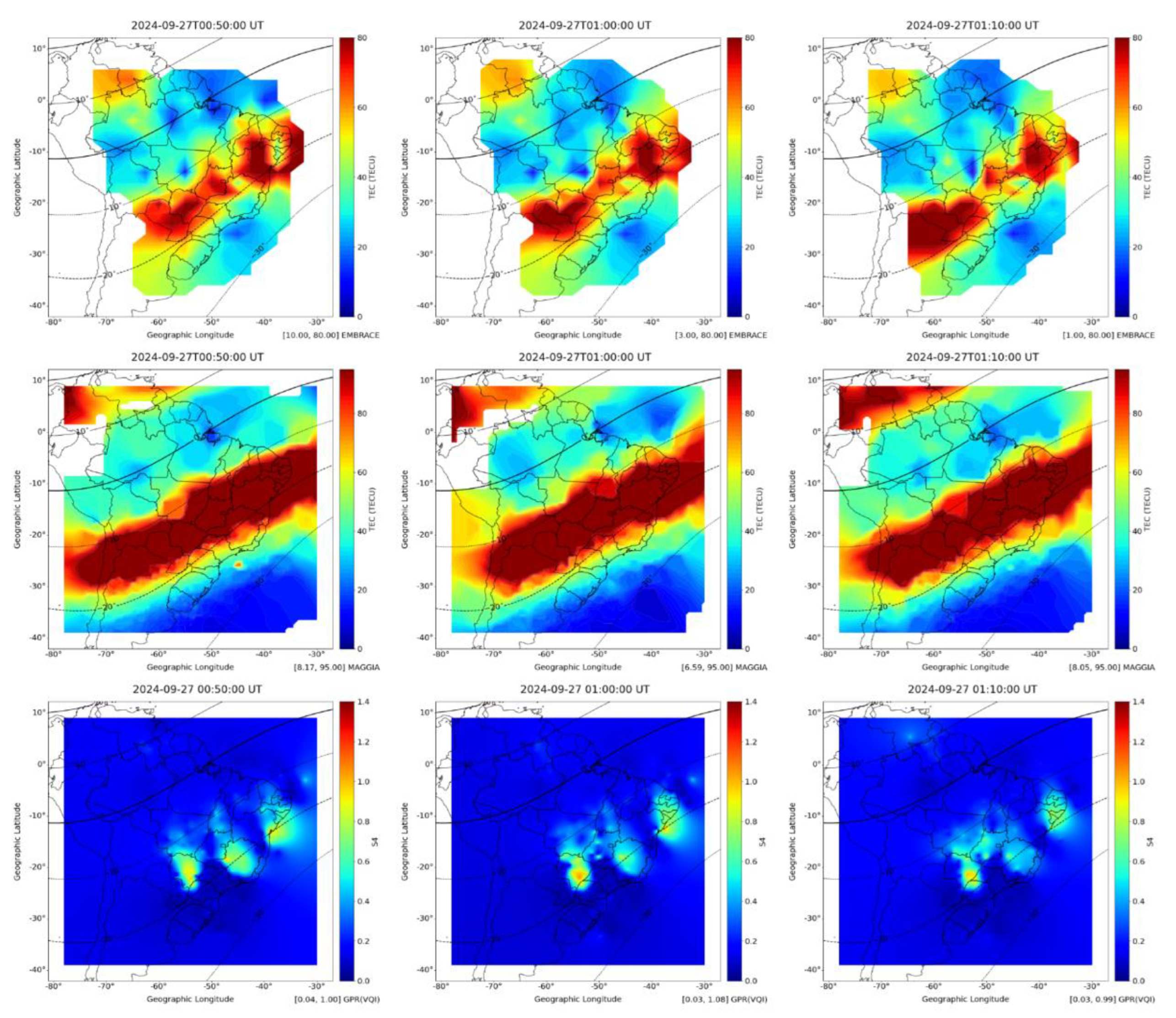
Figure 2.
Flowchart of the adopted methodology, showing the component steps.
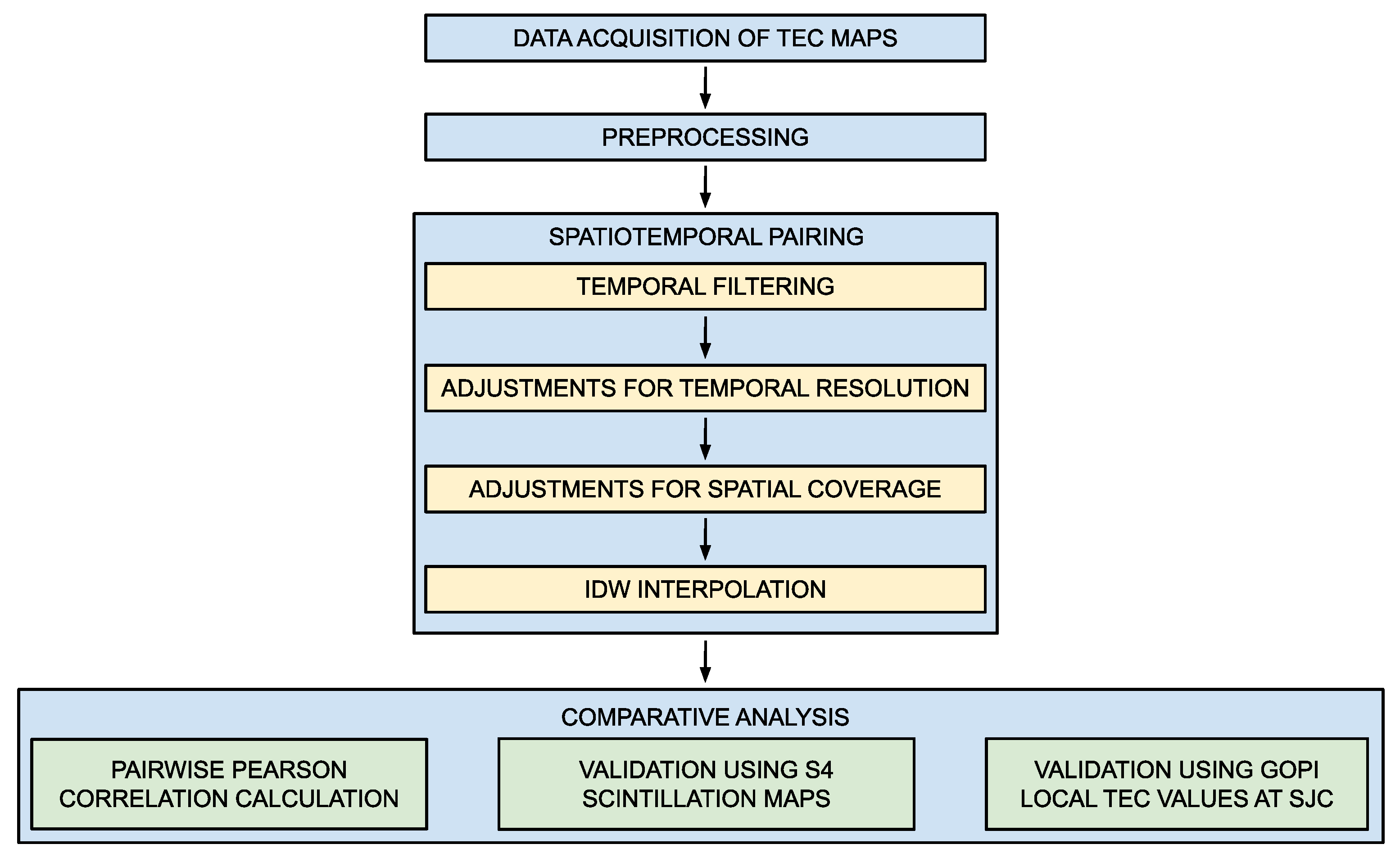

Table 1.
TEC maps sources of this study.
| Source | Spatial resolution (lat x long) |
Temporal resolution (min) |
Spatial coverage |
TEC map extension |
|---|---|---|---|---|
| IGS (https://igs.org/products/#ionosphere) | 2.5° x 5° | 120 | Global | (87.5° S to 87.5° N;180.0° W to 180.0° E) |
| INPE/EMBRACE (https://www2.inpe.br/climaespacial/portal/tec-map-sobre/ / https://www2.inpe.br/climaespacial/portal/tec-map-inicio/) | 2° x 2.5° | 10 | South America | (60.0° S to 20.0° N;90.0° W to 30.0° W) |
| MAGGIA (https://www.maggia.unlp.edu.ar/productos_maggia_alta) | 0.5° x 0.5° | 15 (until 09/04/2024) 10 (since 09/05/2024) |
Central and South America, the Caribbean and Antarctic Peninsula | (80.0° S to 40.0° N;110.0° W to 0°) |
| University of Nagoya (https://stdb2.isee.nagoya-u.ac.jp/GPS/GPS-TEC/index.html) | 0.5° x 0.5° | 5 | Global | (89.9° S to 89.6° N;180.0° W to 180.0° E) |
Table 2.
Temporal coverage of TEC maps (DOY denotes day-of-the-year).
| Source/ Period |
IGS | INPE | MAGGIA | Nagoya |
|---|---|---|---|---|
| March/ 2022 |
Complete | Complete | DOYs 68, 72 and 87 to 89 incomplete | Complete |
| June/ 2022 |
Complete | Complete | DOYs 155, 175, 177, 179 and 180 incomplete |
Complete |
| September/ 2022 |
Complete | Complete | DOYs 244, 257, 259 and 263 incomplete |
Complete |
| December/ 2022 |
Complete | Missing | DOYs 336, 342, 355 and 361 incomplete | DOYs 335 to 337 and 341 to 347 incomplete |
| March/ 2023 |
Complete | Missing | DOYs 60 and 73 incomplete |
Complete |
| June/ 2023 |
Complete | Missing | DOYs 152 to 156 incomplete |
Complete |
| September/ 2023 |
Complete | Missing | DOYs 248, 259 and 261 incomplete | DOYs 251 to 258 incomplete |
| December/ 2023 |
Complete | Missing | DOYs 336, 340, 354 and 364 incomplete | Complete |
| March/ 2024 |
Complete | Complete | DOYs 82 to 85 incomplete |
DOY 90 missing |
| June/ 2024 |
Complete | Complete | DOYs 172, 179 and 182 incomplete | DOYs 178 and 179 incomplete |
| September/ 2024 |
Complete | Complete | DOYs 259, 260 and 273 incomplete |
DOYs 245 and 246 incomplete |
| December/ 2024 |
Complete | DOY 348 incomplete and 366 missing | Complete | Complete |
Table 3.
Comparisons between each pair of TEC sources using TF1 (best value is marked in blue, and the worst, in red).
Table 3.
Comparisons between each pair of TEC sources using TF1 (best value is marked in blue, and the worst, in red).
| Source/ Period |
All months |
03/ 2022 |
06/ 2022 |
09/ 2022 |
03/ 2024 |
06/ 2024 |
09/ 2024 |
12/ 2024 |
|---|---|---|---|---|---|---|---|---|
| IGS x Nagoya | 0.14 | 0.22 | 0.03 | 0.15 | 0.21 | 0.13 | 0.17 | 0.05 |
| IGS x EMBRACE | 0.14 | 0.21 | 0.04 | 0.17 | 0.29 | 0.15 | 0.14 | 0.01 |
| IGS x MAGGIA | -0.05 | 0.08 | -0.33 | -0.15 | 0.16 | -0.18 | 0 | 0.07 |
| EMBRACE x Nagoya | 0.67 | 0.75 | 0.80 | 0.75 | 0.57 | 0.70 | 0.49 | 0.51 |
| EMBRACE x MAGGIA | 0.64 | 0.70 | 0.75 | 0.71 | 0.62 | 0.70 | 0.55 | 0.40 |
| EMBRACE x IGS | 0.14 | 0.21 | 0.04 | 0.17 | 0.29 | 0.15 | 0.14 | 0.01 |
| Nagoya x MAGGIA | 0.62 | 0.68 | 0.77 | 0.66 | 0.59 | 0.68 | 0.50 | 0.43 |
| Nagoya x IGS | 0.14 | 0.22 | 0.03 | 0.15 | 0.21 | 0.13 | 0.17 | 0.05 |
| Nagoya x EMBRACE | 0.67 | 0.75 | 0.80 | 0.75 | 0.57 | 0.70 | 0.49 | 0.51 |
| MAGGIA x Nagoya | 0.62 | 0.68 | 0.77 | 0.66 | 0.59 | 0.68 | 0.50 | 0.43 |
| MAGGIA x EMBRACE | 0.64 | 0.70 | 0.75 | 0.71 | 0.62 | 0.70 | 0.55 | 0.40 |
| MAGGIA x IGS | -0.05 | 0.08 | -0.33 | -0.15 | 0.16 | -0.18 | 0 | 0.07 |
Table 4.
Correlations between each pair of TEC sources using TF2 (best value is marked in blue, and the worst, in red).
Table 4.
Correlations between each pair of TEC sources using TF2 (best value is marked in blue, and the worst, in red).
| Source/ Period |
All months |
12/ 2022 |
03/ 2023 |
06/ 2023 |
09/ 2023 |
12/ 2023 |
|---|---|---|---|---|---|---|
| IGS x Nagoya | 0.20 | 0.23 | 0.25 | 0.12 | 0.20 | 0.17 |
| IGS x MAGGIA | 0.02 | 0.20 | 0.08 | -0.23 | -0.07 | 0.13 |
| Nagoya x MAGGIA | 0.65 | 0.65 | 0.69 | 0.72 | 0.67 | 0.47 |
| Nagoya x IGS | 0.20 | 0.23 | 0.25 | 0.12 | 0.12 | 0.20 |
| MAGGIA x Nagoya | 0.65 | 0.65 | 0.69 | 0.72 | 0.67 | 0.47 |
| MAGGIA x IGS | 0.02 | 0.20 | 0.08 | -0.23 | -0.07 | 0.13 |
Table 5.
Correlations between each pair of TEC sources using TF3 only for TEC values equal or above Q3 (best value is marked in blue, and the worst, in red).
Table 5.
Correlations between each pair of TEC sources using TF3 only for TEC values equal or above Q3 (best value is marked in blue, and the worst, in red).
| Source/Period | 03/2024 | 06/2024 | 09/2024 | 12/2024 |
|---|---|---|---|---|
| EMBRACE x Nagoya | 0.23 | 0.26 | 0.17 | 0.26 |
| Nagoya x EMBRACE | 0.13 | 0.76 | 0.11 | 0.15 |
| EMBRACE x MAGGIA | 0.36 | 0.46 | 0.33 | 0.30 |
| MAGGIA x EMBRACE | 0.18 | 0.05 | 0.10 | 0.16 |
| Nagoya x MAGGIA | 0.32 | 0.51 | 0.22 | 0.19 |
| MAGGIA x Nagoya | 0.19 | 0.40 | 0.13 | 0.13 |
Table 6.
Correlations between each pair of TEC sources using TF3 for TEC values equal or above Q3 or the full range, shown as the first and second values in each cell, respectively (best value is marked in blue, and the worst, in red).
Table 6.
Correlations between each pair of TEC sources using TF3 for TEC values equal or above Q3 or the full range, shown as the first and second values in each cell, respectively (best value is marked in blue, and the worst, in red).
| Source/Period | 03/2024 | 06/2024 | 09/2024 | 12/2024 |
|---|---|---|---|---|
| EMBRACE x All | 0.64 / 0.29 | 0.73 / 0.36 | 0.56 / 0.25 | 0.46 / 0.27 |
| MAGGIA x All | 0.67 / 0.18 | 0.72 / 0.21 | 0.59 / 0.10 | 0.43 / 0.14 |
| Nagoya x All | 0.62 / 0.23 | 0.72 / 0.31 | 0.54 / 0.15 | 0.47 / 0.17 |
Table 7.
Comparison of TEC local values for SJC between Gopi (± standard deviation), EMBRACE and MAGGIA for the chosen times of September 27th, 2024 (values in TECU).
Table 7.
Comparison of TEC local values for SJC between Gopi (± standard deviation), EMBRACE and MAGGIA for the chosen times of September 27th, 2024 (values in TECU).
| Source/Time | 00:50 UT | 01:00 UT | 01:10 UT |
|---|---|---|---|
| Gopi | 30.89 ± 19.69 | 30.06 ± 11.62 | 29.8 ± 7.92 |
| EMBRACE | 30.45 | 30.20 | 27.33 |
| MAGGIA | 51.22 | 50.70 | 47.56 |
Table 8.
Comparison of TEC local values for SJC between Gopi (± standard deviation), IGS, Nagoya, EMBRACE and MAGGIA for the four higher TEC values observed in the Gopi time series for December, 2024, at 15 LT (values in TECU).
Table 8.
Comparison of TEC local values for SJC between Gopi (± standard deviation), IGS, Nagoya, EMBRACE and MAGGIA for the four higher TEC values observed in the Gopi time series for December, 2024, at 15 LT (values in TECU).
| Source/Time | 12/18/2024 | 12/22/2024 | 12/19/2024 | 12/01/2024 |
|---|---|---|---|---|
| Gopi | 71.73 ± 5.98 | 67.49 ± 4.86 | 67.35 ± 2.73 | 67.11 ± 2.09 |
| IGS | 93.81 | 91.86 | 83.63 | 93.43 |
| Nagoya | 81.89 | 81.10 | 76.48 | 78.39 |
| EMBRACE | 80.40 | 78.20 | 77.22 | 78.46 |
| MAGGIA | 81.64 | 86.52 | 80.77 | 87.67 |
Table 9.
Comparison of TEC local values for SJC between Gopi (± standard deviation), Nagoya, EMBRACE and MAGGIA for the four peak values observed in the Gopi time series for December, 2024, and the corresponding days/times (values in TECU).
Table 9.
Comparison of TEC local values for SJC between Gopi (± standard deviation), Nagoya, EMBRACE and MAGGIA for the four peak values observed in the Gopi time series for December, 2024, and the corresponding days/times (values in TECU).
| Source/ Date-Time |
12/18/2024 at 15:20 LT |
12/18/2024 at 15:10 LT |
12/18/2024 at 15:30 LT |
12/18/2024 at 15:00 LT |
|---|---|---|---|---|
| Gopi | 73.49 ± 8.34 | 73.19 ± 7.07 | 72.30 ± 10.16 | 71.73 ± 5.98 |
| Nagoya | 81.76 | 84.34 | 81.30 | 81.89 |
| EMBRACE | 81.15 | 80.70 | 82.63 | 80.40 |
| MAGGIA | 83.16 | 82.30 | 84.15 | 81.64 |
Disclaimer/Publisher’s Note: The statements, opinions and data contained in all publications are solely those of the individual author(s) and contributor(s) and not of MDPI and/or the editor(s). MDPI and/or the editor(s) disclaim responsibility for any injury to people or property resulting from any ideas, methods, instructions or products referred to in the content. |
© 2025 by the authors. Licensee MDPI, Basel, Switzerland. This article is an open access article distributed under the terms and conditions of the Creative Commons Attribution (CC BY) license (http://creativecommons.org/licenses/by/4.0/).
Copyright: This open access article is published under a Creative Commons CC BY 4.0 license, which permit the free download, distribution, and reuse, provided that the author and preprint are cited in any reuse.


