
Submitted:
10 June 2025
Posted:
12 June 2025
You are already at the latest version
Abstract
This study explores the use of deep learning models with attention mechanisms for predicting multiple soil properties from multi-temporal Sentinel-2 satellite images. We developed and tested two convolutional neural network architectures: one with a shared attention layer for all target properties, and another with separate attention layers for each property. The models were trained and evaluated on data from 45.000 locations across the United States. The main goal was to analyze which satellite bands and months are most relevant for soil property regression, as identified by the learned attention weights. In additional experiments, we excluded the most important bands to test their impact on prediction accuracy. The results show that attention mechanisms help highlight relevant input features and that removing key bands generally reduces model performance. To the best of our knowledge, such a direct integration of attention mechanisms with regression models for multi-temporal Sentinel-2-based soil property mapping has not been previously reported. This approach provides insight into model behavior and may support future applications in remote sensing-based soil analysis.
Keywords:
soil properties
; remote sensing
; Sentinel-2
; explainable AI
; attention
; multi-target regression
1. Introduction
A crucial, non-renewable natural resource, soil serves as the basis for both human civilization and terrestrial ecosystems. It serves as the foundation for plant growth, offers habitat to innumerable creatures, and is crucial in controlling the cycles of carbon, nutrients, and water that are necessary for ecosystem health and agricultural output [1]. Soil is a property created at the Earth’s surface by the combined effect of parent material, climate, water, topography, flora, and fauna, and consisting of a complex and dynamic mixture of minerals, organic matter, water, air, and living beings [2]. A variety of soil types, each with distinct physical and chemical characteristics, are produced by this special composition and the processes that shape it.
The significance of soil goes much beyond its use in agriculture. In addition to being a natural habitat for plants and animals, soil also acts as a filter and groundwater storage facility, a medium for the breakdown and recycling of organic waste, and a crucial regulator of climate and atmospheric gases [3]. Therefore, soil is essential for food security as well as for preserving environmental quality and ecosystem services as well.
The ability of the soil to promote productivity, maintain ecological functions like carbon sequestration and nutrient cycling, and support plant and microbial life is reflected in the broader notion of soil health, which is becoming more widely acknowledged [4]. Strong plant growth, biological diversity, and resource efficiency are all made possible by healthy soils. Conversely, soil degradation brought on by pollution, erosion, compaction, or salinization can drastically lower ecosystem resilience and productivity [5].
The function and health of soil are largely dependent on its physical (texture, structure, porosity, and bulk density), chemical (pH and nutrient content), and biological (microbial activity and organic matter concentration) qualities [6]. Soil fertility, water retention, aeration, root development, and the capacity to sustain a variety of biological communities are all directly impacted by these characteristics. For instance, soil structure affects aeration and root penetration, whereas soil texture controls drainage and water retention [7]. Organic matter-rich soils, such mollisols and alfisols, have high fertility and they are among the most productive for agriculture due to their ability to retain water [8]. On the other hand, degraded soils or entisols, which have little nutrient content or weak structure, may need significant management inputs to sustain productivity [9]. Modifications to these characteristics that can drastically impact crop yields and ecological resilience, such as decreased aggregation or increased compaction [10].
Thus, knowledge of and control over soil characteristics are crucial for long-term ecosystem health, sustainable agriculture, and management of this priceless asset.
Soil is essential for maintaining crops as well as for controlling hydrological processes, filtering pollutants, and storing carbon, all of which support environmental health and climate regulation [8].
Sustainable soil management techniques, including crop rotation, cover crops, conservation tillage, and organic amendments, are strongly advocated as ways to combat degradation. It has been demonstrated that these methods promote nitrogen cycling, boost organic matter, improve soil structure, and encourage beneficial microbial activity [11].
Sustainable soil stewardship is crucial in light of global issues including land degradation, climate change, and the rising need for food. Long-term agricultural productivity, environmental quality, and future generations’ access to food depend on preserving and improving soil health [12].
Research Objectives
Since neural networks are frequently "black boxes," the goal is to determine which Sentinel-2 image input features—bands and periods—have the biggest impact on soil property prediction. As a result, consumers benefit from more openness, less data is needed for future applications, and models with different sources can be used (drones, more satellites) with a restricted number of channels.
2. Background and Related Work
Recent developments in artificial intelligence (AI) have completely changed the agricultural industry and ushered in the era of Agriculture 5.0, where precision agriculture is made possible by the convergence of interconnected technologies like robotics, remote sensing, the Internet of Things (IoT), and advanced data analytics [13].
In order to maximize crop management, resource allocation, and yield prediction, these AI-driven systems analyze enormous volumes of real-time data from a variety of sources, including weather stations, satellite imaging, soil sensors, and unmanned aerial vehicles. Using deep learning models and machine learning (ML), these days, agronomists and farmers may make data-driven, well-informed decisions that boost food systems’ resilience to climate change, increase productivity, and lessen their negative effects on the environment [13].
Even though contemporary AI models are remarkably predictive, interpretability and transparency have become increasingly problematic due to their growing complexity, especially as deep learning architectures like Long Short-Term Memory (LSTM) networks have become more widely used. These alleged "black box" devices frequently don’t have the ability to give concise, intelligible justifications for their results, which may prevent them from being used in high-stakes industries like agriculture where responsibility, trust, and regulatory compliance are crucial [14]. A strong framework for explainability is required since the opacity of AI models is particularly troublesome in situations when judgments affect resource distribution, land management, or environmental stewardship [14].
The goal of Explainable Artificial Intelligence (XAI), a crucial field, is to demystify the sophisticated AI systems’ decision-making processes. The goal of XAI is to provide both global insights into model behavior and local, instance-specific justifications for individual predictions. Examples of these techniques include SHapley Additive exPlanations (SHAP), Local Interpretable Model agnostic Explanations (LIME), Permutation Importance (PI), and Partial Dependence Plots (PDP) [14,15].
These techniques help stakeholders comprehend the directionality of their effects, the relative relevance of input attributes, consider the ways in which factors interact, therefore encouraging more trust in suggestions generated by AI [15].
The General Data Protection Regulation (GDPR), which requires the right to an explanation for automated choices that impact humans, is one regulatory framework that XAI is essential to guaranteeing compliance with [14].
XAI has several different applications in agriculture. Explainability, in general, helps farmers, agronomists, and policymakers to examine, verify, and improve AI-driven insights by bridging the gap between sophisticated analytics and real-world field application [13].
Transparent models allow for cooperative communication between human expertise and machine intelligence, which empowers stakeholders to identify abnormalities, pose important queries, and customize treatments for particular agro-ecological settings [14]. XAI improves the accountability and transparency of suggestions for crop selection, fertilizer application, pest control, and irrigation scheduling in smart farming applications, ultimately promoting more effective and sustainable farming methods [13].
With a particular focus on soil parameter estimate, XAI is essential for a number of reasons. Plant development, ecosystem function, and climate regulation are all based on the characteristics of the soil, including temperature, moisture, organic carbon content, and nutrient availability [16]. To maximize input use, these characteristics must be estimated accurately in order to enhance productivity projections and reduce environmental hazards. However, advanced modeling techniques are required due to the complexity and heterogeneity of soil systems as well as the large dimensionality of sensor and remote sensing data. Researchers and practitioners can analyze model predictions using XAI techniques, determine which environmental characteristics are most influential, then evaluate if the linkages that have been learned are consistent with accepted soil science principles [16].
For example, research using XAI to predict soil temperature has shown that air temperature and radiation are the main factors, and that model transparency improves the accuracy and usefulness of prediction tools for soil management [16]. Furthermore, by exposing data biases, identifying erroneous correlations, and pointing out regions that require more data collection or domain knowledge integration, XAI helps to continuously enhance soil models [13,16]. In addition to increasing model accuracy, this iterative feedback loop guarantees that AI-driven soil parameter estimation stays rooted in physical reality and is flexible enough to accommodate changing problems in agriculture [13,16].
Building trust, complying with regulations, and utilizing the full potential of digital transformation in sustainable soil management will all depend on the integration of XAI as agriculture continues to embrace AI on a large scale [13,14].
Using plant development characteristics, Abekoon et al. [17] created an explainable machine learning model to forecast soil levels of nitrogen (N), phosphorous (P), and potassium (K) in cabbage production. To interpret the model’s predictions, the study used Local Interpretable Model-agnostic Explanations (LIME) and SHapley Additive exPlanations (SHAP), increasing the AI system’s openness and credibility.
Over the course of 85 days, the researchers gathered data from cabbage plants cultivated in the Sri Lanka’s central hills. The model’s inputs included important plant characteristics like the number of leaves, plant height, average leaf area, and number of days. Higher plant height and leaf count had a favorable effect on the prediction of soil nutrient levels, according to SHAP research, however more days and a bigger average leaf area had a negative effect. In addition to providing thorough interpretations for individual forecasts, LIME offered instance-specific explanations, validating the global insights from SHAP.
15 greenhouse-grown cabbage plants at different stages of growth were examined in order to validate the model, and the actual measurements and the anticipated nutrient levels nearly matched.
Kakhani et al. [18] used XAI to improve the interpretability of soil organic carbon (SOC) prediction models, addressing a rising requirement in digital soil mapping. Although machine learning techniques like Random Forests (RF) have demonstrated encouraging results in simulating SOC, their opaqueness sometimes restricts their applicability in research and policymaking. In order to clarify the inner workings of SOC prediction models trained on environmental factors, this study constructed SHAP.
The scientists trained RF models to predict SOC using data from two different sites in England. They then used SHAP to calculate the relative contributions of each input variable, such as soil depth, topography, remote sensing indices, and land cover. In addition to confirming the predominance of factors like elevation and soil depth, SHAP also showed subtle feature interactions that would otherwise go undetected in conventional feature importance scores.
Interestingly, the study showed that improving model explainability did not result in a decrease in prediction accuracy.
The interpretability of convolutional neural networks (CNNs) in the context of digital soil mapping (DSM) is examined in a study by Beucher et al. [19], which focuses on the classification of acid sulfate (AS) soils in Denmark’s Jutland wetlands.
Using a dataset of 5,885 labeled soil samples and 14 optimized environmental covariates derived via recursive feature elimination, the authors evaluate CNNs and Random Forest models for binary classification of possible AS soil occurrence. CNNs perform marginally better than RFs in terms of prediction accuracy (68% vs. 61–63%), but their main contribution is the effective use of SHAP to show the local and spatial effects of variables. Key indicators identified by the study include detrended DEM, depth to pre-Quaternary deposits and the distance to the Littorina Sea shoreline. Beucher et al. demonstrate how spatial variables grouped in image-like patches can supply CNNs with contextual information, enabling a more detailed representation of environmental gradients.
Beucher et al. show that CNNs can benefit from contextual information provided by spatial covariates arranged in image-like patches, allowing for a more nuanced representation of environmental gradients.
In order to increase the accuracy of crop output forecasts, Mohan et al. [20] investigate the merging of artificial intelligence and explainable AI. The authors stress that although AI techniques like random forest models, deep neural networks, and support vector machines are frequently used in agriculture, their interpretability issues still pose a obstacle to further adoption. The authors created a hybrid prediction system that uses SHAP and LIME for model interpretability and a Deep Neural Network for yield prediction. By combining crop management information, soil characteristics (pH, organic content), and meteorological parameters (rainfall, temperature, and humidity), they applied this approach to a dataset with over 10,000 occurrences spread over several growing regions.
The DNN model outperformed other machine learning models including Random Forest (MAPE = 9.83%) and SVM (MAPE = 11.27%), with a Mean Absolute Percentage Error (MAPE) of 7.56% and an R2 score of 0.92. These findings show that intricate, nonlinear relationships between environmental elements and agricultural productivity more efficiently can be captured by deep learning architectures.
Crucially, the authors employed SHAP to pinpoint and illustrate the main forces influencing the DNN’s predictions. For example, average soil nitrogen levels, rainfall during the flowering period, and the variations in temperature throughout the vegetative phase were consistently found to be the most significant characteristics in all regional models. Higher rainfall variability had a detrimental effect on yield, as demonstrated by SHAP summary plots, whereas stable nitrogen levels were associated with high production in a positive way.
Additionally, localized explanations for individual forecasts were produced using LIME, providing assistance in the interpretation of anomalies, such as surprisingly poor yields in fields with otherwise ideal circumstances.
In order to improve agricultural decision-making processes in contexts with limited data and high risk, Shams et al. [21] look into the use of XAI to improve crop recommendation systems. Despite their strong predictive capabilities, the authors contend that traditional AI models employed for crop recommendations frequently lack interpretability, which undermines farmers’ and agronomists’ confidence and practical implementation.
The study presents an integrated system that combines SHAP for interpretability with an optimized Extreme Gradient Boosting (XGBoost) model for classification. A real-world dataset from Egypt’s agricultural zones was used to train the model. This dataset included information on crop yield history, soil type, pH, rainfall, temperature, and levels of nitrogen, phosphorus, and potassium.
Performance-wise, the XGBoost model with classification accuracy of 96.2
The authors explained the model’s recommendations both locally and globally using SHAP. The top three criteria determining crop recommendations, according to the global SHAP research, were temperature range, yearly rainfall, and soil nitrogen concentration. For instance, rice recommendations were mostly linked to high rainfall and slightly acidic soil (pH 6.0), but wheat was heavily preferred under moderate nitrogen and low rainfall conditions. To illustrate how the model modified suggestions in response to subtle variations in feature values, local SHAP explanations were applied to particular case studies. These individualized explanations demonstrated how sensitive the model was to slight changes in the pH or potassium content of the soil, providing farmers with useful information about how to apply soil amendments.
Additionally, the study evaluated the interpretability of the domain-specific explanations from specialists. According to a user assessment, 85% of agronomists thought SHAP plots were useful for comprehending the recommendations for certain crops, suggesting that XAI-enhanced decision support tools have a lot of promise for real-world use.
A study on the application of XAI techniques in combination with LSTM networks to improve the precision and comprehensibility of soil temperature prediction models is presented by Geng et al. [22]. Agricultural planning, irrigation scheduling, and seed germination all depend on accurate soil temperature predictions, but standard models frequently fail to account for nonlinear and temporal correlations in environmental data.
The authors of this study created an LSTM-based model that was trained over a five-year period using a dataset that included soil and weather data from five distinct Chinese regions. Air temperature, relative humidity, solar radiation, wind speed, and soil moisture content were important input characteristics. With a coefficient of determination (R²) of 0.92, and a Root Mean Square Error (RMSE) of 1.18°C, the LSTM model showed good predictive ability, surpassing conventional models like Random Forest (RMSE = 1.65°C) and Support Vector Regression (RMSE = 2.07°C).
The authors used SHAP to examine how each input feature contributed to the model’s output in order to overcome the interpretability issue. According to SHAP values, air temperature accounted for more than half of the predictive power, making it the most important element. Soil moisture and solar radiation came in second and third, respectively. Curiously, the impact of wind speed and relative humidity differed greatly by season, underscoring how feature relevance in time series models depends on context.
To gain a better understanding of the LSTM’s basic logic, temporal SHAP value analysis was also employed to illustrate how each feature’s effect changed across various time steps. This method improved the understanding of model sensitivity to extreme weather events and allowed researchers to identify aberrant prediction patterns.
AgroXAI, a novel crop recommendation system that combines XAI with machine learning algorithms to improve decision-making in the context of Agriculture 4.0, is introduced by Turgut et al. [23]. The study tackles a prevalent issue in intelligent agricultural systems: although AI models provide accurate forecasts, their opaqueness undermines user confidence and restricts practical implementation among farmers and agronomists.
An XGBoost model trained on a curated dataset of 7,000 Turkish agricultural records is used by the AgroXAI framework. These data contain characteristics like the type of soil, climatic zone, pH, precipitation, average temperature, and concentrations of macronutrients (NPK).
The model suggests the best crops (such as wheat, corn, sunflower, and cotton) based on the agro-environmental characteristics of a particular area. With an accuracy of 97.6%, the XGBoost model outperformed other models that were examined, including Random Forests (94.8%) and Decision Trees (91.4%).
The system combines SHAP and LIME to provide recommendations both locally and internationally, increasing transparency. According to the SHAP analysis, the most important variables influencing all of the suggestions were pH levels, precipitation patterns, and soil nitrogen levels. For example, the model consistently recommended cotton in warmer, high-nitrogen, low-precipitation zones and wheat in areas with moderate nitrogen and slightly alkaline soil (pH 7–7.5). LIME was used to produce case-specific interpretations that explain the recommendations for specific crops under a specific input combination.
Using data from unmanned aerial vehicles (UAVs), Kumar et al. [24] describe a solid study aimed at enhancing corn yield prediction by combining ML models and XAI approaches. The necessity for both interpretability and high-accuracy forecasting in actual agricultural situations is what motivates the research.
Using multispectral UAV footage, the authors gathered red, green, blue, red-edge, and near-infrared) over Ontario, Canada’s cornfields in the growth seasons of 2022 and 2023. A variety of vegetation indices (NDVI, GNDVI, NDRE, etc.) were created to act as input features for modeling once ground truth yield data was captured at harvest.
Random Forest, Gradient Boosting Machines (GBM), and XGBoost were the tested models. XGBoost performed the best, outperforming RF (R2 = 0.88) and GBM (R2 = 0.87), with an R2 of 0.91 and an RMSE of 0.46 t/ha. Recursive feature elimination was used to choose the input characteristics, which included canopy temperature, solar radiation, and vegetation indices.
The authors used SHAP to analyze model predictions in order to address interpretability. The two most important factors in yield estimation, according to the worldwide SHAP summary, were canopy temperature and NDRE (Normalized Difference Red Edge Index). Higher mid-season NDRE values, for instance, were favorably associated with yield, whereas higher canopy temperatures during the reproductive stages were associated with lower production as a result of heat stress. Targeted management decisions were made possible by the researchers’ ability to identify yield-affecting conditions at the plot level using local SHAP plots. For example, in several instances, concurrently high canopy temperature caused high NDVI values to result in unexpectedly low yield forecasts; this realization was made feasible by SHAP interaction effects.
To the best of our knowledge, while several research have used attention mechanisms in image analysis or regression models for predicting soil properties, the combination of attention mechanisms and regression models for multitemporal the mapping of soil properties using Sentinel-2 has never been documented in the literature before.
3. Materials and Methods
3.1. Description of the Data
The data used in this study were collected from a total of 45,000 different locations covering the entire area of the United States during 2023. The locations were randomly generated throughout the USA, and for each, data on soil properties and satellite images were collected. For each geolocation, values are available for 55 soil properties, as well as 12 monthly Sentinel-2 images.
To preserve quality and consistency, all locations that did not have complete data on all soil properties were excluded from the analysis. At this stage, no additional filters were applied, such as selection by land cover type or altitude.
Soil property data were obtained from the California Soil Resource Laboratory [25] at UC Davis University and are based on current USDA-NCSS data obtained from official field surveys. Properties are aggregated within square cells of 800 m2.
Available soil properties are classified into three main categories:
- Chemical properties: calcium carbonate, cation exchange capacity (CEC), pH value, soil organic matter, sodium adsorption ratio, electrical conductivity
- Physical properties: bulk density, sand content, silt content, clay content, saturated hydraulic conductivity, rock fragments, soil texture
- Land use related properties: depth to restrictive layer, wind erodibility index, soil depth, hydrologic group, land capability class, wind erodibility group, soil order, soil temperature regime
The complete list of all available soil properties, with those used in this study (✓) specially marked, is given in Table 1.
For a complete description of each property, see Appendix A.
Satellite Data
For each location, 12 satellite images are provided – one for each month during 2023. Sentinel-2 (Level-1C) images were used, which enable multispectral analysis of the land surface with high spatial resolution. Each satellite image covers a square area of 400 × 400 meters (which corresponds to an image resolution of 40 × 40 pixels per location). For each image, all relevant spectral channels of the Sentinel-2 mission (13 bands in total) are available.
Note:
- Channels in the visible and near-infrared spectrum (B02–B08) are key for vegetation and soil status analysis.
- SWIR channels (B11 and B12) are useful for moisture detection and soil type classification.
- Red edge channels (B05, B06, B07) are especially valuable for monitoring vegetation stress.
- B09 and B10 are most often used for atmospheric correction but may contain useful information for specific tasks.
For a complete description of each band, see Appendix B.
3.2. Data Preprocessing
Dynamic augmentation during training. During training, for each location and in each iteration, samples are generated dynamically: from the original image of 40x40 pixels, 32x32 pixels are randomly selected, and the selected pixels are randomly permuted and arranged in a new image of the same dimensions. This augmentation method is applied in every batch during training, which increases data diversity and efficiently reduces overfitting.
Target data are normalized in the range 0–1.
3.3. Model Architecture
In this research, we used two deep learning models based on convolutional neural networks, with an added attention mechanism that helps the model “focus” on the most important input data. These models are trained to predict several different soil properties at the same time, using both satellite images and field measurements.
The first model, attention-merge, uses a single shared attention layer for all target properties. This means the model finds which satellite channels and months are most important for predicting all soil properties together.
The second model, attention-split, has a separate attention layer for each soil property. In this way, the model can learn which data is most important for each property individually, which makes the results more precise and easier to interpret.
Figure 1 shows both models: on the left is the model with shared attention for all properties, and on the right is the model that uses separate attention for each property.
In both architectures, the attention layer is implemented as a Dense layer with sigmoid activation that generates weights for all input channels and months, which are then applied to the input data by element-wise multiplication.
3.4. Model Training
Training was conducted in two successive phases with the aim of thoroughly examining the importance of input data for model performance.
Phase 1: In the first phase, each of the models (attention-merge and attention-split) was trained 100 times, using the Adam optimizer with a learning rate of 0.001, batch size of 64, for 128 epochs (with 32 batches per epoch). In each of the 100 experiments (trainings), the sample set was randomly split into training, validation, and test sets in a 60:20:20 ratio. Trainings were performed on a workstation with an Intel Core i5-13600 processor, 64 GB RAM, and NVIDIA RTX 3090 GPU. TensorFlow and Keras were used for implementation and experimentation.
After completion of the first phase, the attention layers were analyzed to identify input bands and time periods (months) that have the highest significance for the model in predicting soil properties. This analysis enables the detection of input data that "stand out" as most informative.
Phase 2: In the second phase, all previously identified input bands and months (those with the highest attention coefficients) were omitted from the new training process. The models were then retrained and evaluated with the same settings, to assess whether their exclusion causes a statistically significant deterioration in training quality, i.e., the ability to regress the output (measured) parameters.
Note: The aim of the experimental design is not to achieve maximum model performance but to isolate and confirm the importance of individual input data. The number of epochs and training size were chosen to enable as much experiment replication and reliable statistical estimation of importance as possible, even at the cost of slightly compromised maximum accuracy metrics. The key value of this approach is the confirmation that the exclusion of attention-identified bands indeed leads to a reduction in the model’s ability to learn the appropriate relations, thus confirming their key role in the model.
4. Results and Discussion
Figure 2 shows the training process for the attention-merge model across 100 repeated experiments. Blue lines represent training loss, and red lines represent validation loss for each experiment.
It can be seen that the training (validation) loss has not reached its minimum and there is still plenty of room for optimization. For now, it is important to state that in the planned 128 episodes, no overfitting occurred.
Figure 3 and Figure 4 show the Normalized Mean Absolute Error (NMAE) and R2 metric for all observed properties. The graphs show results for both models (attention-merge and attention-split), obtained as the mean from 100 independent experiments with 128 epochs per experiment. For comparison, results are also shown when each model was trained only once for 2048 epochs, to assess the longer-term trend of performance.
Figure 5 shows the heatmap of the attention scores obtained from the attention layer of the attention-mergee model, showing the dependence between months and satellite bands based on the average from 100 repeated experiments.
It can be noticed that bands B09 (Water vapor, 945 nm) and B10 (Short-wave infrared, cirrus, 1375 nm) stand out the most, and to some extent B12 (Short-wave infrared, 2190 nm) and B01 (Coastal aerosol, 443 nm). The dominance of these channels can be explained by their sensitivity to the physical-chemical properties of the soil and the presence of moisture. B09 (water vapor) and B10/B12 (shortwave infrared region) are particularly significant because the SWIR range provides important information on soil moisture content, texture, the presence of mineral matter, and organic components. B10 (cirrus) is extremely sensitive to water vapor and moisture, which may be directly related to agricultural potential and soil condition. B01 (coastal aerosol) can contribute to the detection of surface particles, dust, and other aerosols, which indirectly affects surface soil properties.
In Figure 6(1/2),(2/2), heatmaps are shown for the attention layer for each soil property individually for the attention-split model. In most maps, bands B09 and B10 are still the most pronounced, while B11 and B12 are somewhat less represented. For certain properties, such as electrical conductivity and sodium adsorption ratio, RGB channels also play a significant role, especially during the middle of the calendar year.
In the second phase, during the training of the attention-merge model, channels B09 and B10 were excluded from the input data, and the entire training procedure was repeated under the same conditions as in the previous experiments. Figure 7 shows comparative results for Normalized Mean Absolute Error (NMAE) values, trained with all channels and without channels B09 and B10, based on the mean from 100 repeated experiments. For each soil property, the 95% confidence interval is also shown, allowing a clearer assessment of the importance of individual channels for model performance.
Looking at the chart 7, which shows results for the attention-merge model, it is clear that for 11 of the total 17 shown soil properties, there is no overlap of the confidence intervals between the model trained with all channels and the model trained without channels B09 and B10. This further confirms the findings from the previous heatmap and indicates the importance of these channels for model accuracy. Interestingly, in the setting where one attention layer is used for all soil properties at the same time, excluding channels B09 and B10 leads to improvement only in one property (sodium adsorption ratio), while for the other properties it either worsens performance or a reliable conclusion cannot be drawn from the shown data.
5. Conclusions
In this research, we analyzed which spectral channels from Sentinel-2 satellite images and in which months contribute the most to the estimation of soil properties using deep neural networks. Two architectures were tested: a model with a shared attention layer (attention-merge) and a model with separate attention layers for each target (attention-split) variable individually. The results showed, somewhat surprisingly, that the greatest influence among the input data is from bands B09 (Water vapor, 945 nm) and B10 (Short-wave infrared, cirrus, 1375 nm). Regarding seasonal dependence, it is not possible to unequivocally highlight a certain month, but it can be observed that satellite images from the middle of the calendar year are generally more important for the prediction of soil properties.
To confirm the findings obtained from the analysis of attention layer values, attention-merge model was further trained after excluding the most significant channels (B09 and B10). The results achieved show that such exclusion significantly reduces model accuracy, confirming the key role of these channels in the prediction process.
To draw final conclusions, further research is needed, including systematic removal of other, less significant channels, to assess their contribution and enable further optimization of the amount and structure of input data. This would create the basis for even more efficient models, adapted to limited resources or application to other satellites and sensors.
Acknowledgments
Parts of this manuscript were prepared with the assistance of ChatGPT (OpenAI, 2025), which was used for language editing, grammar and style correction, database and reference search, and text refinement. ChatGPT was also occasionally used for technical assistance with code implementation; however, all research ideas, model design, data analysis, programming logic, experimentation, and scientific interpretation were conceived and performed solely by the authors. The authors reviewed and approved the final content.
Conflicts of Interest
The authors declare that they have no conflict of interest.
Appendix A. Soil Properties: Detailed Description
Description of soil properties and their application
Soil properties represent key parameters for understanding the chemical composition, physical structure, and potential of soil for various uses. Each characteristic has its specific application, both in agriculture and in ecology, engineering, and environmental protection:
Chemical properties:
- Calcium Carbonate (CaCO3): Amount of calcium carbonate in the soil. The presence of limestone is important for neutralizing soil acidity and determining overall fertility. Soils with high concentrations of CaCO3 are often alkaline, which can affect the availability of phosphorus and micronutrients.
- Cation Exchange Capacity (CEC): Measure of the soil’s ability to retain and exchange nutrient cations (e.g., Ca2+, Mg2+, K+, Na+). High CEC indicates a greater ability of the soil to retain nutrients and resistance to degradation.
- Electrical Conductivity (EC): Soil electrical conductivity, an indicator of total dissolved salts. High values indicate salinity that can endanger plant growth. EC is used to detect degradation and determine the need for reclamation.
- pH: Indicator of soil acidity or alkalinity. It affects nutrient availability, microorganism activity, and chemical processes in the soil. Optimal pH values (usually 6–7) allow maximum nutrient use.
- Sodium Adsorption Ratio (SAR): The ratio of sodium concentration to other cations in the soil. High SAR can cause degradation of soil structure, reduced permeability, and increased risk of erosion.
- Soil Organic Matter (SOM): The presence of organic matter (humus) increases fertility, water retention capacity, aggregate stability, and soil recovery.
Physical properties:
- Available Water Holding Capacity (AWHC): The soil’s ability to retain water available to plants. Key for assessing crop drought resistance and irrigation planning.
- Bulk Density: Soil density (mass per unit volume). Lower values indicate loose and well-aerated soil, while high values may indicate compaction and poor water infiltration.
- Rock Fragments: Content of larger mineral particles and stones affects mechanical workability, water infiltration capacity, and overall soil productivity.
- Saturated Hydraulic Conductivity: The ability of the soil to conduct water when fully saturated. Key for drainage and prevention of excess water retention in the root zone.
- Sand, Silt, Clay: The granulometric composition of the soil determines soil texture (sandy, loamy, clayey) and capacity to retain water and nutrients.
Land use related properties:
- Depth To Restrictive Layer: Depth to a layer (e.g., rock, hard clay) that limits root growth and water flow. Greater depth allows better plant development.
- Kw Factor 0–25 cm: Wind erodibility factor for the surface soil layer, important for assessing the risk of erosion.
- Soil Depth: The total depth of the soil profile. Deeper soils usually have greater capacity for water and nutrients.
- Wind Erodibility Index: Index of soil susceptibility to wind erosion, important for planning protection and preserving the surface layer.
The significance of all these properties is reflected in the ability for precise fertility assessment, planning optimal agrotechnical measures, identifying degraded areas, and improving soil resource conservation strategies.
Appendix B. Sentinel-2 Bands: Technical Details and Applications
Detailed descriptions of each Sentinel-2 spectral band with practical application:
- B01 (443 nm, 60 m, Blue): This band is primarily intended for aerosol detection and estimation of atmospheric turbidity, which is crucial for correct interpretation of satellite data and precise atmospheric correction. Used for correction of reflected signals in water surfaces and vegetation. Due to low spatial resolution, used mainly as an auxiliary band in atmosphere.
- B02 (490 nm, 10 m, Blue): High spatial resolution enables detailed mapping of surface waters, detection and monitoring of clouds, snow, and ice cover. Extremely important in urban areas and for monitoring ecologically sensitive zones such as lakes and rivers. Often used for recognizing land-water boundaries.
- B03 (560 nm, 10 m, Green): The green band is key for basic vegetation analysis, including calculation of vegetation indices (NDVI, GNDVI). Enables detection of healthy and stressed plant communities. Also suitable for mapping land cover and monitoring terrain changes.
- B04 (665 nm, 10 m, Red): The most important band for calculating NDVI (Normalized Difference Vegetation Index), the standard for assessing photosynthetic activity and overall vegetation health. This band allows distinguishing between actively growing vegetation and non-vegetated soil, and is indispensable in agricultural and ecological monitoring.
- B05 (705 nm, 20 m, Red edge): The first red edge band in the Sentinel-2 series. Particularly sensitive to changes in chlorophyll content and can detect early signs of plant stress, invisible in classical visible bands. Used for monitoring crop phenological phases and detection of diseases or nutrient deficiencies.
- B06 (740 nm, 20 m, Red edge): Builds on B05 and allows even more precise assessment of changes in vegetation. Especially important for monitoring forest ecosystems, land degradation, and agricultural crops. Contributes to the analysis of vegetation cover structure and quality.
- B07 (783 nm, 20 m, Red edge): Used to assess total plant biomass, detect fires, and monitor vegetation regeneration after fires or degradation. Enables detailed mapping of permanent grasslands and forests. Often combined with B05 and B06 for advanced vegetation indices.
- B08 (842 nm, 10 m, Near-IR): The most important band for vegetation analysis. Near-IR reflects energy on healthy plants and enables very precise distinction of vegetation from non-vegetated surfaces (e.g., water, soil). Extremely useful for detection of soil moisture and flood areas, as well as for assessing vegetation cover density.
- B8A (865 nm, 20 m, Narrow Near-IR): This band enables more detailed segmentation of vegetation and is used for monitoring boundaries between vegetation and water surfaces, as well as for assessing changes in wetlands and coastal zones. Combined with B08 gives even more precise results in mapping biological and hydromorphological changes.
- B09 (945 nm, 60 m, Water vapor): Specific band designed for detection of water vapor content in the atmosphere. Essential for correction of atmospheric influence in the analysis of reflected signals, which increases the accuracy of multispectral analyses of soil and vegetation.
- B10 (1375 nm, 60 m, SWIR–Cirrus): Enables detection of cirrus clouds and assessment of the influence of high, thin clouds on image quality. Helps in automatic selection and filtering of scenes with undesirable atmospheric conditions, which is crucial for obtaining reliable data in time series.
- B11 (1610 nm, 20 m, SWIR): Shortwave infrared band used for analysis of soil and vegetation moisture, as well as for identification of mineral surface composition. Important for classification of soil types, detection of degradation, and determination of clay or sand content in soil.
- B12 (2190 nm, 20 m, SWIR): The furthest band in the SWIR domain of Sentinel-2 mission, used for estimation of total surface moisture, land cover classification, detection of forest and surface fires, as well as erosion and land degradation. Enables detection of changes not visible in visible or NIR spectrum.
References
- Food and Agriculture Organization of the United Nations. Soil is a non-renewable resource, 2015. Accessed: 2025-05-28.
- University of Minnesota Extension. Five factors of soil formation, 2025. Accessed: 2025-05-28.
- Natural Resources Conservation Service, USDA. Soil Health, 2025. Accessed: 2025-05-28.
- Fausak, L.K.; Bridson, N.; Diaz-Osorio, F.; Jassal, R.S.; Lavkulich, L.M. Soil health–a perspective. Frontiers in Soil Science 2024, 4, 1462428. [Google Scholar] [CrossRef]
- Derpsch, R.; Kassam, A.; Reicosky, D.; Friedrich, T.; Calegari, A.; Basch, G.; Gonzalez-Sanchez, E.; dos Santos, D.R. Nature’s laws of declining soil productivity and Conservation Agriculture. Soil Security 2024, 14, 100127. [Google Scholar] [CrossRef]
- NC State Extension. Soil Physical Health, 2025. Accessed: 2025-05-28.
- Noble Research Institute. Soil and Water Relationships, 2022. Accessed: 2025-05-28.
- Needelman, B.A. Soil: The Foundation of Agriculture. Nature Education Knowledge 2013, 4, 2. [Google Scholar]
- Li, T.; Cui, L.; Filipović, V.; Tang, C.; Lai, Y.; Wehr, B.; Song, X.; Chapman, S.; Liu, H.; Dalal, R.C.; et al. From soil health to agricultural productivity: The critical role of soil constraint management. Catena 2025, 250, 108776. [Google Scholar] [CrossRef]
- Longepierre, M.; Widmer, F.; Hartmann, M. Limited resilience of the soil microbiome to mechanical compaction within four growing seasons of agricultural management. ISME Communications 2021, 1, 1–10. [Google Scholar] [CrossRef] [PubMed]
- Shahane, A.A.; Shivay, Y.S. Soil health and its improvement through novel agronomic and innovative approaches. Frontiers in Agronomy 2021, 3, 680456. [Google Scholar] [CrossRef]
- Kopittke, P.M.; Menzies, N.W.; Wang, P.; McKenna, B.A.; Lombi, E. Soil and the intensification of agriculture for global food security. Environment international 2019, 132, 105078. [Google Scholar] [CrossRef] [PubMed]
- Oliveira, R.C.d.; Silva, R.D.d.S.e. Artificial intelligence in agriculture: benefits, challenges, and trends. Applied Sciences 2023, 13, 7405. [Google Scholar] [CrossRef]
- Hrast Essenfelder, A.; Toreti, A.; Seguini, L. Expert-driven explainable artificial intelligence models can detect multiple climate hazards relevant for agriculture. Communications Earth & Environment 2025, 6, 207. [Google Scholar]
- Astolfi, D.; De Caro, F.; Vaccaro, A. Recent advances in the use of explainable artificial intelligence techniques for wind turbine systems condition monitoring. Electronics 2023, 12, 3509. [Google Scholar] [CrossRef]
- Novielli, P.; Magarelli, M.; Romano, D.; Di Bitonto, P.; Stellacci, A.M.; Monaco, A.; Amoroso, N.; Bellotti, R.; Tangaro, S. Leveraging explainable AI to predict soil respiration sensitivity and its drivers for climate change mitigation. Scientific Reports 2025, 15, 12527. [Google Scholar] [CrossRef] [PubMed]
- Abekoon, T.; Sajindra, H.; Rathnayake, N.; Ekanayake, I.U.; Jayakody, A.; Rathnayake, U. A novel application with explainable machine learning (SHAP and LIME) to predict soil N, P, and K nutrient content in cabbage cultivation. Smart Agricultural Technology 2025, 11, 100879. [Google Scholar] [CrossRef]
- Kakhani, N.; Taghizadeh-Mehrjardi, R.; Omarzadeh, D.; Ryo, M.; Heiden, U.; Scholten, T. Towards explainable AI: interpreting soil organic carbon prediction models using a learning-based explanation method. European Journal of Soil Science 2025, 76, e70071. [Google Scholar] [CrossRef]
- Beucher, A.; Rasmussen, C.B.; Moeslund, T.B.; Greve, M.H. Interpretation of convolutional neural networks for acid sulfate soil classification. Frontiers in Environmental Science 2022, 9, 809995. [Google Scholar] [CrossRef]
- Mohan, R.J.; Rayanoothala, P.S.; Sree, R.P. Next-gen agriculture: integrating AI and XAI for precision crop yield predictions. Frontiers in Plant Science 2025, 15, 1451607. [Google Scholar] [CrossRef] [PubMed]
- Shams, M.Y.; Gamel, S.A.; Talaat, F.M. Enhancing crop recommendation systems with explainable artificial intelligence: a study on agricultural decision-making. Neural Computing and Applications 2024, 36, 5695–5714. [Google Scholar] [CrossRef]
- Geng, Q.; Wang, L.; Li, Q. Soil temperature prediction based on explainable artificial intelligence and LSTM. Frontiers in Environmental Science 2024, 12, 1426942. [Google Scholar] [CrossRef]
- Turgut, Ö.; Kök, İ.; Özdemir, S. AgroXAI: Explainable AI-Driven Crop Recommendation System for Agriculture 4.0. In Proceedings of the 2024 IEEE International Conference on Big Data (BigData). IEEE; 2024; pp. 7208–7217. [Google Scholar]
- Kumar, C.; Dhillon, J.; Huang, Y.; Reddy, K. Explainable machine learning models for corn yield prediction using UAV multispectral data. Computers and Electronics in Agriculture 2025, 231, 109990. [Google Scholar] [CrossRef]
- Walkinshaw, M.; O’Geen, A.; Beaudette, D. Soil properties. California Soil Resource Lab, 1 Oct 2022, 2023.
Figure 1.
Schematic overview of used models. (a) Attention-merge: shared attention layer for all outputs. (b) Attention-split: independent attention layers, one for each output variable.
Figure 1.
Schematic overview of used models. (a) Attention-merge: shared attention layer for all outputs. (b) Attention-split: independent attention layers, one for each output variable.
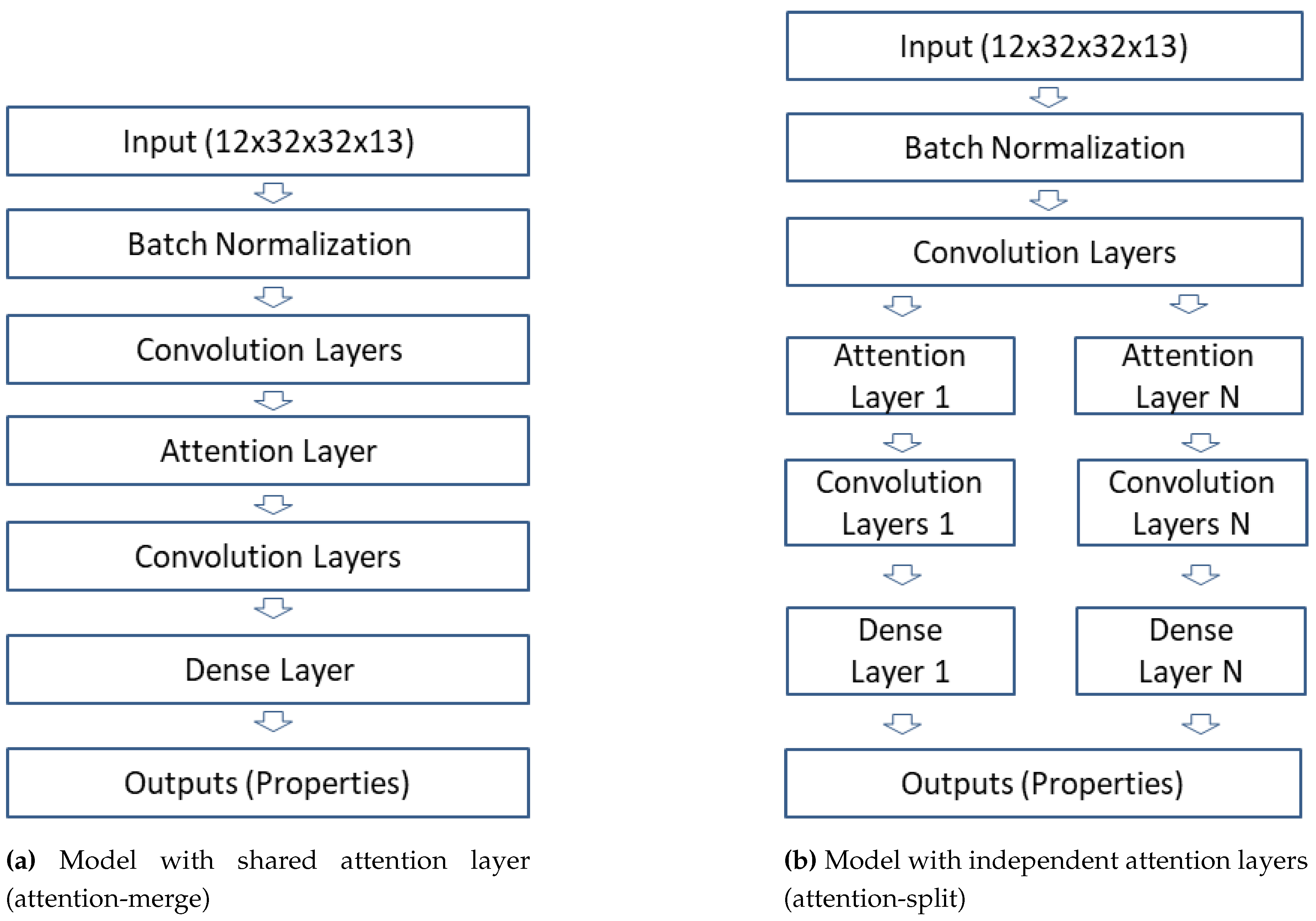
Figure 2.
Training and Validation loss.
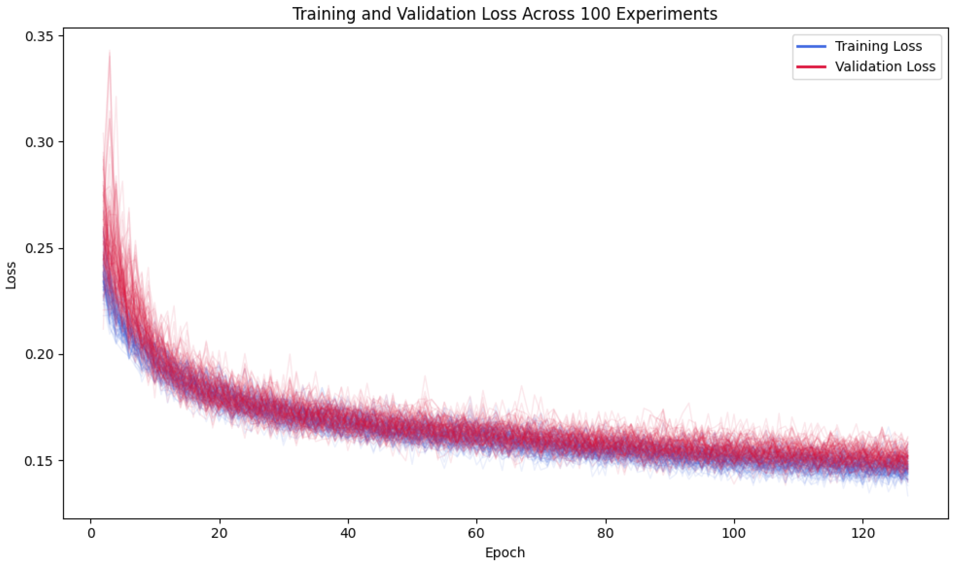
Figure 3.
Normalized Mean Absolute Error.
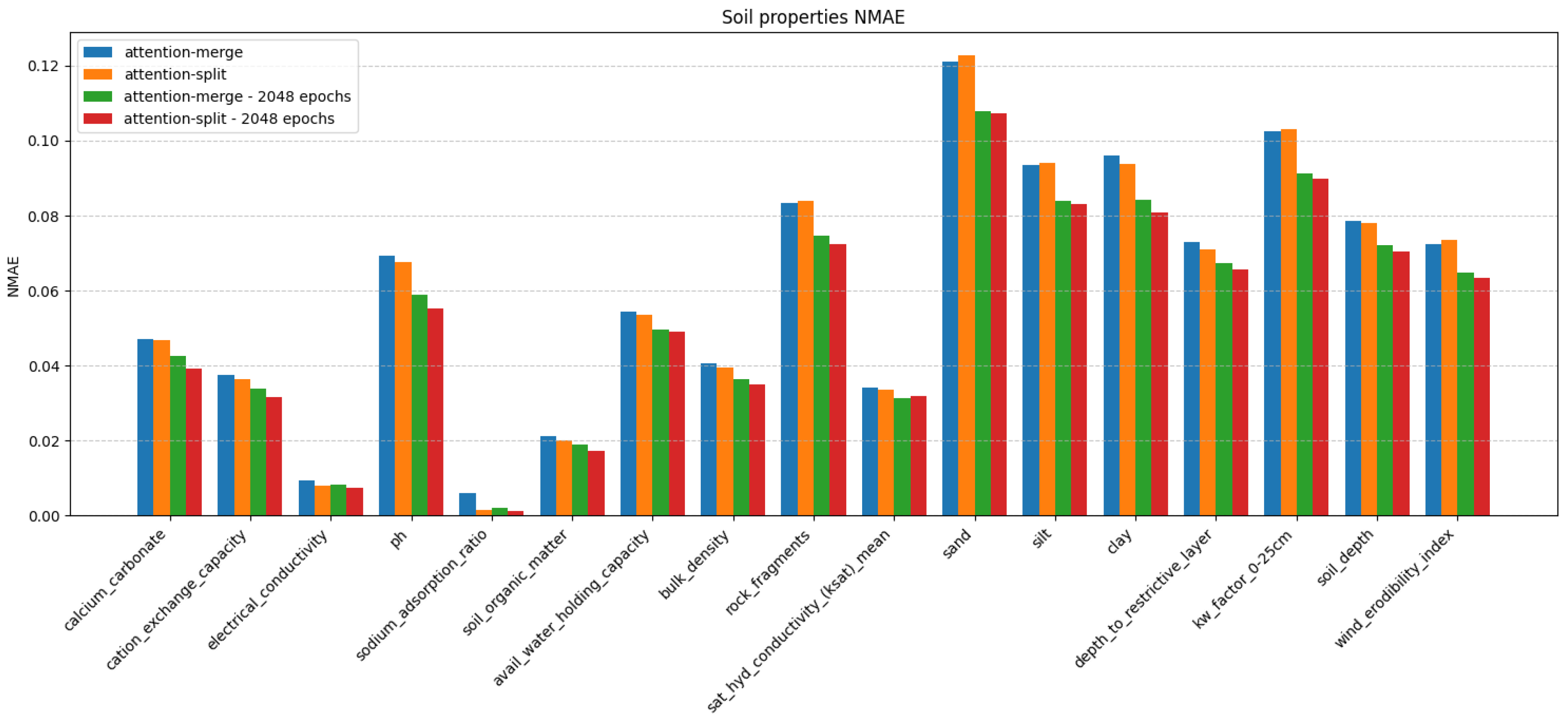
Figure 4.
R2 metric.
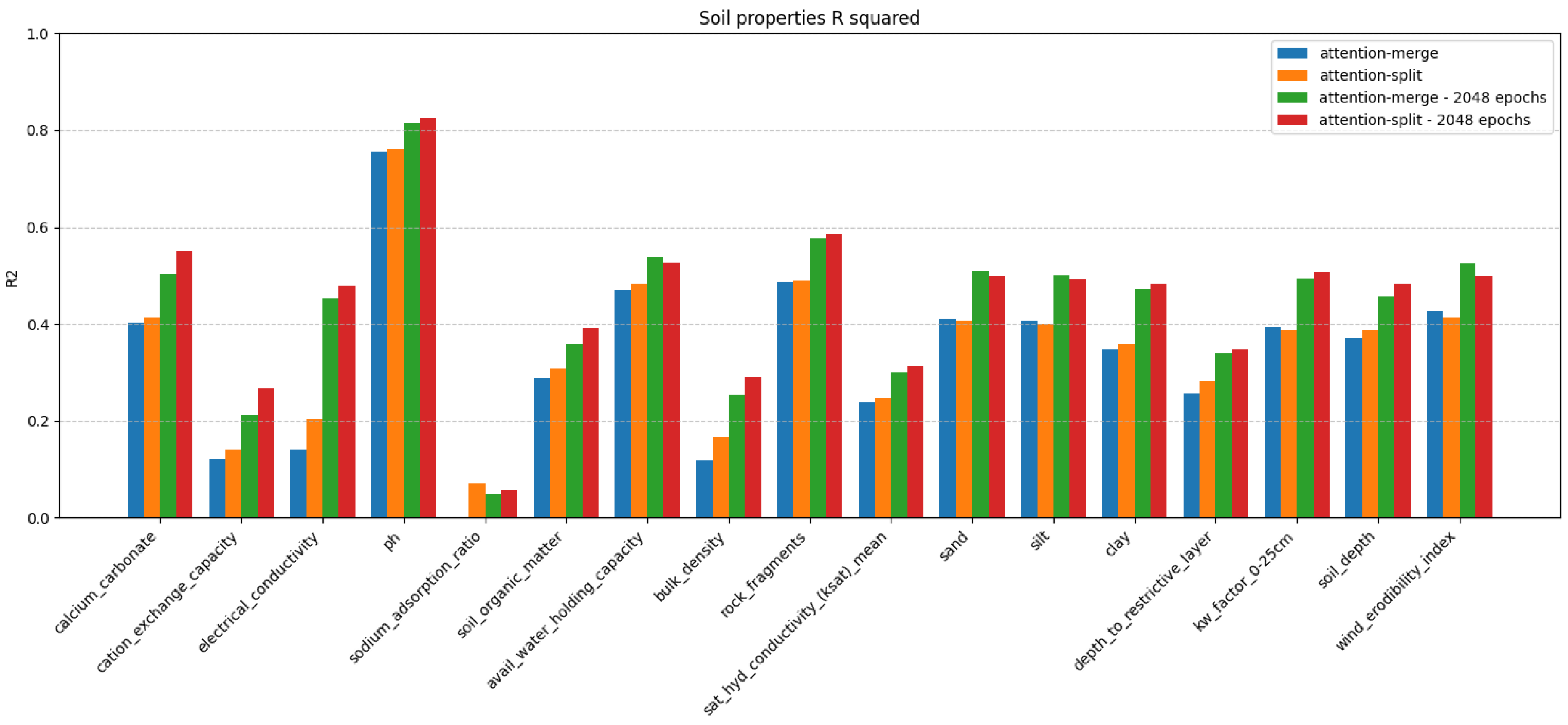
Figure 5.
Heat map for Attention Scores.
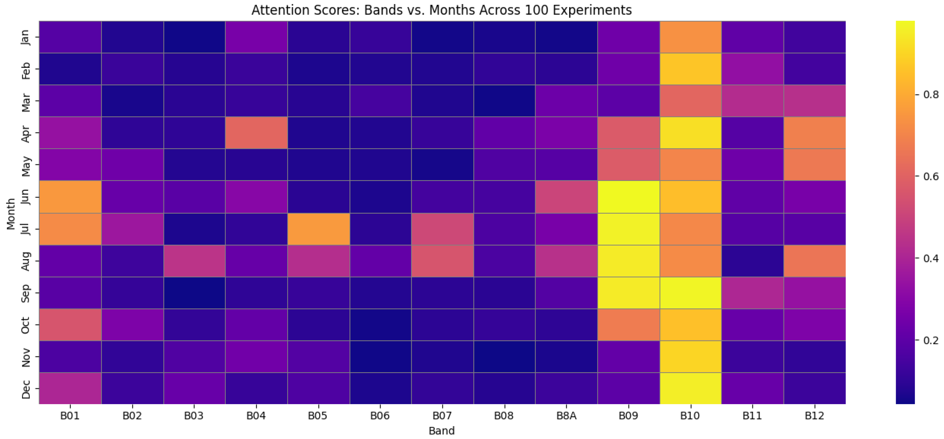
Figure 6.
(1/2). Soil property maps (1/2): First 8 properties. (2/2). Soil property maps (2/2): Remaining 9 properties.
Figure 6.
(1/2). Soil property maps (1/2): First 8 properties. (2/2). Soil property maps (2/2): Remaining 9 properties.
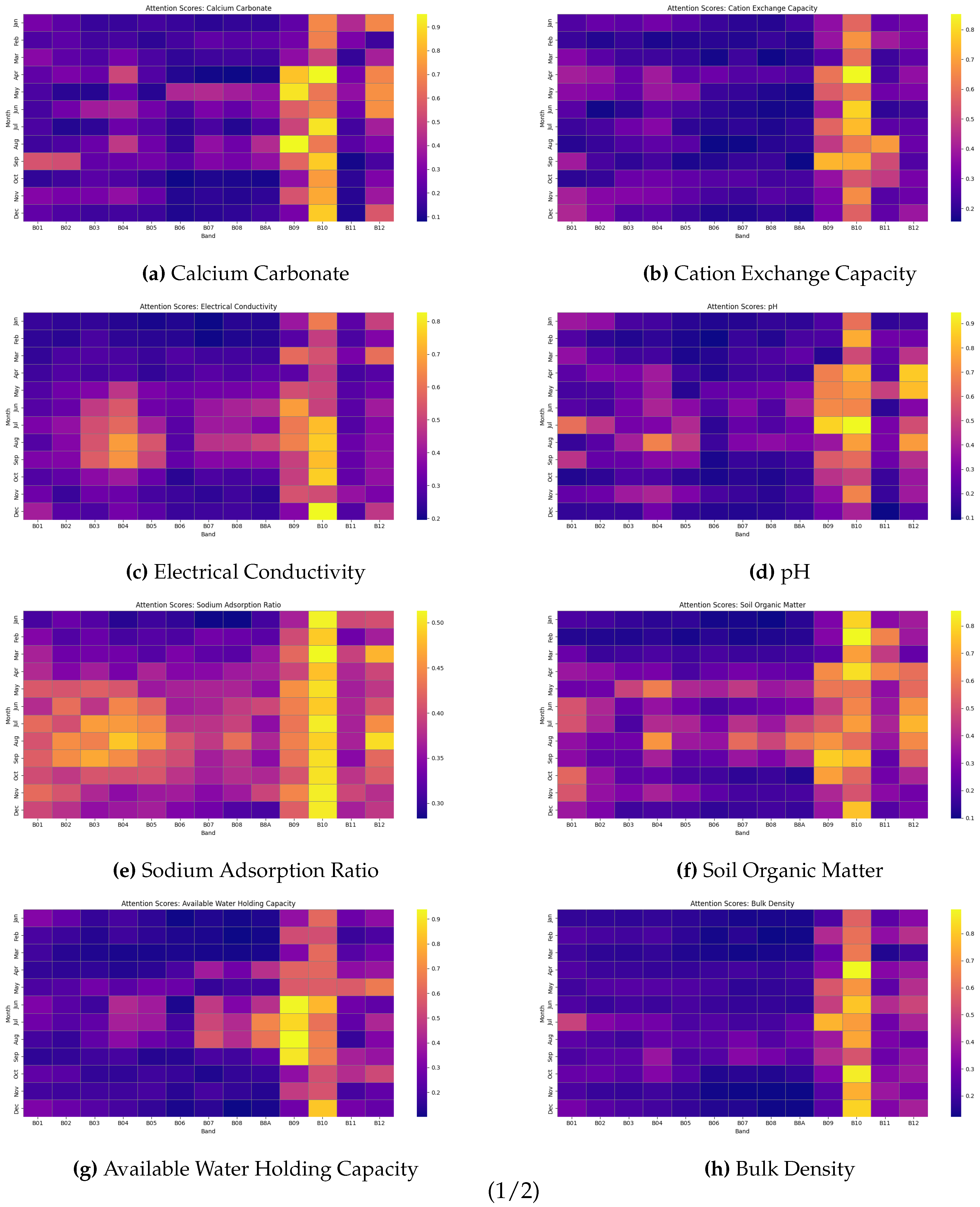
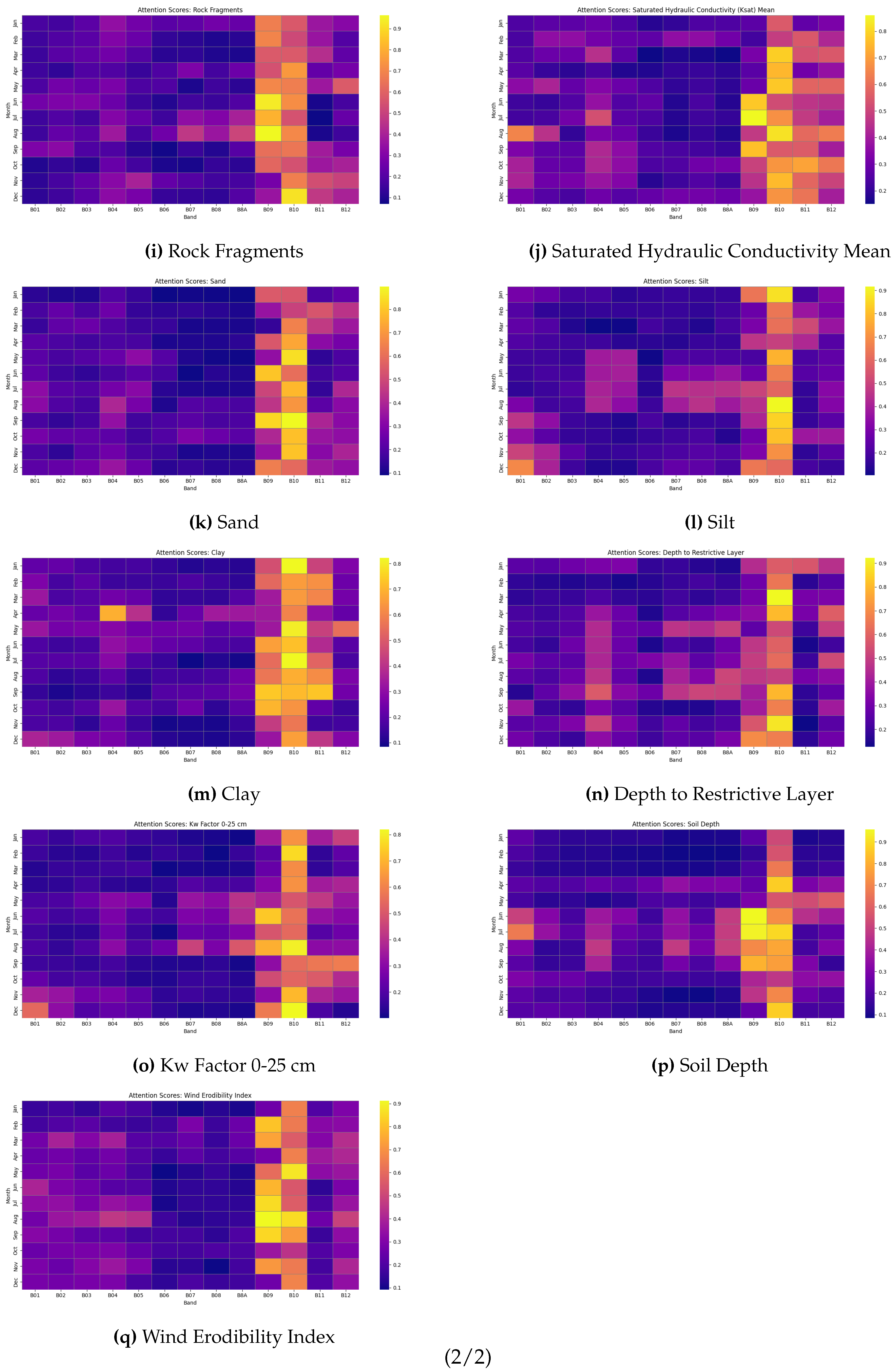
Figure 7.
NMAE for attention-merge model with Full Band Spectrum and Excluding B09 & B10.
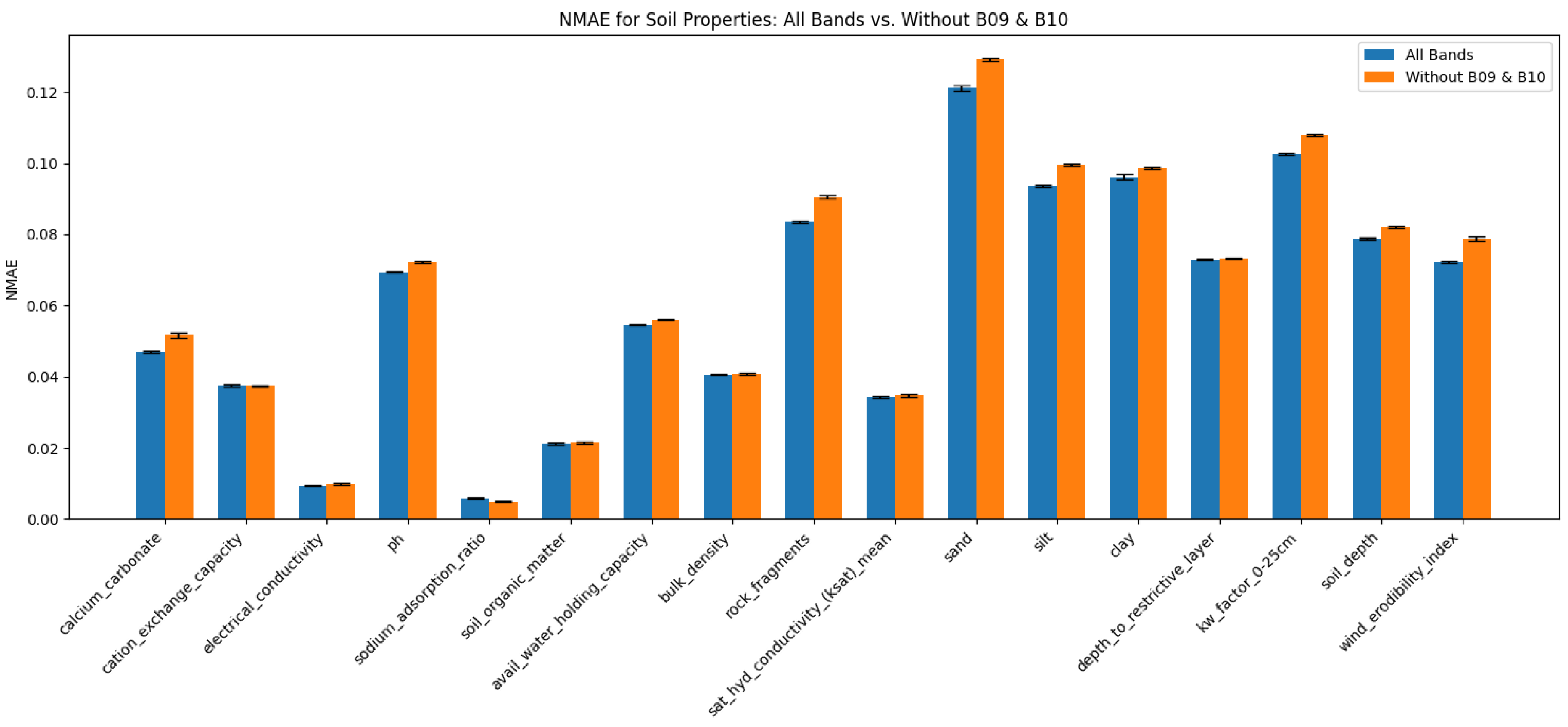

Table 1.
Overview of all available and used soil properties. Properties used in this study are marked with ✓.
Table 1.
Overview of all available and used soil properties. Properties used in this study are marked with ✓.
| No. | Property Name | Category | Data Type | Used |
|---|---|---|---|---|
| 1 | Calcium Carbonate | Chemical | Numeric | ✓ |
| 2 | Cation Exchange Capacity | Chemical | Numeric | ✓ |
| 3 | Cation Exchange Capacity 0-5 cm | Chemical | Numeric | |
| 4 | Cation Exchange Capacity 0-25 cm | Chemical | Numeric | |
| 5 | Cation Exchange Capacity 0-50 cm | Chemical | Numeric | |
| 6 | Electrical Conductivity | Chemical | Numeric | ✓ |
| 7 | Electrical Conductivity 0-5 cm | Chemical | Numeric | |
| 8 | Electrical Conductivity 0-25 cm | Chemical | Numeric | |
| 9 | PH | Chemical | Numeric | ✓ |
| 10 | PH 0-5 cm | Chemical | Numeric | |
| 11 | PH 0-25 cm | Chemical | Numeric | |
| 12 | PH 25-50 cm | Chemical | Numeric | |
| 13 | PH 30-60 cm | Chemical | Numeric | |
| 14 | Sodium Adsorption Ratio | Chemical | Numeric | ✓ |
| 15 | Soil Organic Matter | Chemical | Numeric | ✓ |
| 16 | Soil Organic Matter Max | Chemical | Numeric | |
| 17 | Available Water Holding Capacity | Physical | Numeric | ✓ |
| 18 | Available Water Holding Capacity 0-25 cm | Physical | Numeric | |
| 19 | Available Water Holding Capacity 0-50 cm | Physical | Numeric | |
| 20 | Bulk Density | Physical | Numeric | ✓ |
| 21 | Drainage Class | Physical | Categorical | |
| 22 | Rock Fragments | Physical | Numeric | ✓ |
| 23 | Saturated Hydraulic Conductivity Mean | Physical | Numeric | ✓ |
| 24 | Saturated Hydraulic Conductivity Min | Physical | Numeric | |
| 25 | Saturated Hydraulic Conductivity Max | Physical | Numeric | |
| 26 | Saturated Hydraulic Conductivity 0-5 cm | Physical | Numeric | |
| 27 | Soil Texture 0-5 cm | Physical | Categorical | |
| 28 | Soil Texture 0-25 cm | Physical | Categorical | |
| 29 | Soil Texture 25-50 cm | Physical | Categorical | |
| 30 | Sand | Physical | Numeric | ✓ |
| 31 | Sand 0-5 cm | Physical | Numeric | |
| 32 | Sand 0-25 cm | Physical | Numeric | |
| 33 | Sand 25-50 cm | Physical | Numeric | |
| 34 | Sand 30-60 cm | Physical | Numeric | |
| 35 | Silt | Physical | Numeric | ✓ |
| 36 | Silt 0-5 cm | Physical | Numeric | |
| 37 | Silt 0-25 cm | Physical | Numeric | |
| 38 | Silt 25-50 cm | Physical | Numeric | |
| 39 | Silt 30-60 cm | Physical | Numeric | |
| 40 | Clay | Physical | Numeric | ✓ |
| 41 | Clay 0-5 cm | Physical | Numeric | |
| 42 | Clay 0-25 cm | Physical | Numeric | |
| 43 | Clay 25-50 cm | Physical | Numeric | |
| 44 | Clay 30-60 cm | Physical | Numeric | |
| 45 | Depth To Restrictive Layer | Land Use | Numeric | ✓ |
| 46 | Hydrologic Group | Land Use | Categorical | |
| 47 | Kw Factor 0-25 cm | Land Use | Numeric | ✓ |
| 48 | Land Capability Class Non Irrigated | Land Use | Categorical | |
| 49 | Land Capability Class Irrigated | Land Use | Categorical | |
| 50 | Soil Depth | Land Use | Numeric | ✓ |
| 51 | Soil Order | Land Use | Categorical | |
| 52 | Soil Temperature Regime | Land Use | Categorical | |
| 53 | Wind Erodibility Group | Land Use | Categorical | |
| 54 | Wind Erodibility Index | Land Use | Numeric | ✓ |
| 55 | Survey Type | Land Use | Categorical |
Table 2.
Sentinel-2 spectral bands and their main technical characteristics.
| No. | Band | Central wavelength (nm) | Spatial resolution (m) | Spectral type |
|---|---|---|---|---|
| 1 | B01 | 443 | 60 | Blue |
| 2 | B02 | 490 | 10 | Blue |
| 3 | B03 | 560 | 10 | Green |
| 4 | B04 | 665 | 10 | Red |
| 5 | B05 | 705 | 20 | Red edge |
| 6 | B06 | 740 | 20 | Red edge |
| 7 | B07 | 783 | 20 | Red edge |
| 8 | B08 | 842 | 10 | Near-IR |
| 9 | B8A | 865 | 20 | Narrow Near-IR |
| 10 | B09 | 945 | 60 | Water vapor |
| 11 | B10 | 1375 | 60 | SWIR–Cirrus |
| 12 | B11 | 1610 | 20 | SWIR |
| 13 | B12 | 2190 | 20 | SWIR |
Disclaimer/Publisher’s Note: The statements, opinions and data contained in all publications are solely those of the individual author(s) and contributor(s) and not of MDPI and/or the editor(s). MDPI and/or the editor(s) disclaim responsibility for any injury to people or property resulting from any ideas, methods, instructions or products referred to in the content. |
© 2025 by the authors. Licensee MDPI, Basel, Switzerland. This article is an open access article distributed under the terms and conditions of the Creative Commons Attribution (CC BY) license (http://creativecommons.org/licenses/by/4.0/).
Copyright: This open access article is published under a Creative Commons CC BY 4.0 license, which permit the free download, distribution, and reuse, provided that the author and preprint are cited in any reuse.


