

Submitted:
10 June 2025
Posted:
11 June 2025
You are already at the latest version
Abstract
To map continental water bodies in the southern Andean region of Arequipa, Peru, using satellite images and machine learning algorithms to generate accurate information to facilitate their monitoring, conservation, and sustainable management. The study employed the CRISP-DM methodology, encompassing six phases: business understanding, data understanding, data preparation, modeling, evaluation, and deployment. Sentinel-2 multispectral satellite imagery was processed using ArcGIS Pro. Three supervised machine learning algorithms (Random Forest [RF], Support Vector Machine [SVM], and K-Nearest Neighbor [KNN]) were trained and tested on raster data to classify features into distinct categories and map inland water bodies. Accuracy was assessed using confusion matrices and random sampling validation points. K-Nearest Neighbor algorithm outperformed RF and SVM, achieving over 74% precision and accuracy in detecting inland water bodies, compared to nearly 70% for the other algorithms. The results demonstrated the feasibility of using high-accuracy machine learning techniques to classify and map inland water bodies, specifically lakes and lagoons, by identifying key features contributing to classification accuracy. This research demonstrates the effectiveness of integrating satellite imagery and machine learning in mapping continental water bodies. Generating detailed spatial data supports informed decision-making for preserving Arequipa's continental water bodies, contributing to sustainable environmental management practices.
Keywords:
machine learning
; water bodies mapping
; remote sensing
; Sentinel-2
; geospatial analysis
; continental water bodies
; k-nearest neighbor
; Random Forest
1. Introduction
Water is a crucial resource in socioeconomic processes and in regulating the environment and its various ecosystems [1]. According to the International Union for Conservation of Nature (IUCN), a significant portion of the Earth's aquatic biome and ecosystems are classified within the sphere of freshwater or continental water bodies, which cover only 2.5% of the Earth's land surface [2]. Surface water is essential for meeting the domestic and industrial demands of human society, including drinking water, agriculture, electricity production, and industrial development [3,4]. In this sense, the National Water Authority (ANA) and the Ministry of the Environment (MINAM) in Peru aim to protect and preserve the quality of freshwater resources, such as lakes, lagoons, rivers, and streams, to ensure their accessibility and sustainability over time [5]. However, significant challenges regarding their availability exist, as these freshwater bodies are constantly threatened by human activities and climate change [6]. Rapid population growth and the increase in mining, industrial, and agricultural activities are the primary causes of damage to water resources, which hinders their proper treatment for drinking water production and impacts the quality of ecosystems [5]. Inefficient water management, over-extraction, and pollution are significant threats to water availability and quality. Additionally, the dynamics and variations of water bodies can impact socio-economic activities and water availability, potentially leading to consequences such as flooding [7].
In this context, detecting, mapping, and monitoring surface water resources can provide valuable information about the extent of water bodies and their dynamics, ensuring the sustainability of water and informing the development of effective water management strategies [3].
Over the last few decades, various approaches have been applied to maps and to monitor water bodies. These can be grouped into traditional methods (in situ methods) and methods based on remote sensors [8]. Remote sensors are cost-effective tools that provide information from satellite images in the form of multispectral images that machine learning algorithms can subsequently classify. Technological advances in Remote Sensing offer a significant advantage, as they enable the complete visualization of the Earth's surface and the acquisition of detailed information about the Earth’s surface through satellite sensors. The observation of satellite images through remote sensing has helped in various aspects, including agriculture, flood assessment, monitoring, forest biomass estimation, and oil pollution detection [9]. Satellites like Sentinel-2 from the European Commission and the European Space Agency's Copernicus program can provide multispectral photography of land surfaces, demonstrating higher accuracy in water body extraction [10]. In this context, researchers combine machine learning algorithms with information from various satellite sensors to identify water bodies, their features, and dynamics in semi-arid environments [7]. Machine learning, a branch of artificial intelligence with learning based on pattern recognition, which is presented as an effective alternative for image classification, the most prominent in the field of land cover being Random Forest (RF), Support Vector Machine (SVM) and Classification and Regression Trees (CART) [11]. Supervised learning algorithms utilize certain labeled instances of training datasets to predict similar datasets [12]. The most common supervised algorithms are decision trees, naïve Bayes (NB), neural networks (NNET), regression, support vector machines (SVM), and ensemble methods [13]. Combining machine learning methods with satellite imagery can provide valuable insights into the state of water bodies and their dynamics.
In this study, the primary objective was to detect and map continental water bodies in Arequipa, a region in the southwestern part of Peru, characterized by its variable climate and arid land surfaces, which contain various rivers and lakes. We combine remote sensing data from Sentinel-2 with supervised machine learning algorithms, such as Random Forest (RF), Support Vector Machine (SVM), and K-nearest Neighbor (KNN), using GIS software to process the information and compare the accuracy of these algorithms for mapping continental water bodies. This study can lead to a better understanding of the quantity and state of continental water bodies in Peru.
2. Materials and Methods
To systematically structure the geospatial data analysis and modeling process, the Cross-Industry Standard Process for Data Mining (CRISP-DM) methodology was adopted. This approach has been widely validated in data mining and machine learning contexts for its flexibility, iterative nature, and practical orientation. CRISP-DM consists of six primary phases: business understanding, data understanding, data preparation, modeling, evaluation, and deployment
2.1. Business Understanding
The Arequipa region covers a territorial area of 63,345.39 km² and is situated in the southwestern part of Peru. It has two natural regions: Coast, where the climate is temperate, cloudy, and very arid due to the extensive sandy pampas; and Sierra, where the climate varies, being dry with little presence of aridity due to the constant rains and cold, while closer to the Andes Mountain range and its large volcanoes. The Arequipa region is characterized by numerous rivers that flow from north to south, carving out valleys and canyons (Figure 1).
2.1.1. Problem Identification
First, it is necessary to address the study's problem. In this case, the problem is defined as the absence of local and national projects that evaluate the effectiveness of machine learning algorithms using multispectral satellite images to map lentic continental water bodies, specifically lakes and lagoons, in the Arequipa region of southern Peru.
Therefore, the study's motivation is to contribute to local and national geospatial research using existing information technologies.
2.1.2. Business Objectives
The business objective is to evaluate the effectiveness of machine learning algorithms to identify inland water bodies from multispectral satellite images. Therefore, the following objectives concerning the business and data are defined.
- Obtain satellite images of the Arequipa region.
- Prepare the satellite images of the Arequipa region so that they can be processed by geospatial analysis software.
- Apply machine learning algorithms to identify lentic continental water bodies in the Arequipa region from multispectral satellite images.
- Evaluate and compare the effectiveness of machine learning algorithms for this task.
2.1.3. Assessment of the Current Situation and Requirements
This project will be developed in a computer lab at the University of Arequipa. To obtain data, access to Google Earth Engine is required [14], an Online platform that combines a vast catalog of satellite images and geospatial data of up to several petabytes, with which analyses can be performed on a planetary scale. This is why adequate storage is necessary to save multispectral satellite images or raster data, which have a storage requirement of at least 1 GB per map, for which an SD storage of at least 8 TB is sufficient. Likewise, geospatial analysis software is necessary for image processing and algorithm training, which is why it uses the ArcGIS Pro platform. ArcGIS Pro is the leading desktop geographic information systems (GIS) application. It provides tools and functions that enable users to efficiently maintain spatial data, generate 2D, 3D, and 4D visualizations, and perform advanced cartographic analysis [15].
2.2. Data Understanding
2.2.1. Data Collection
This project uses multispectral satellite images obtained through Google Earth Engine. This engine contains a vast catalog of satellite images and geospatial data with the capacity for analysis on a planetary scale.
The satellite images obtained are from the multispectral sensors (MSI) of the Sentinel-2 MSI satellites [16] of the European Space Agency (ESA), which are high-resolution, wide-range multispectral image sensors supported by the Copernicus: Earth Monitoring Service.
In total, 273 multispectral satellite images corresponding to the Andes were obtained, which will be our work units.
2.2.2. Data Description
Sentinel-2 MSI captures satellite imagery in 13 spectral bands at different spatial resolutions: 4 bands at 10-meter resolution, 6 bands at 20-meter resolution, and 3 bands at 60-meter resolution. The combination of spectral bands enables various uses, including monitoring vegetation, soil, water cover, inland waterways, and coastal zone observation.
The multispectral satellite images presented in this project are raster data. According to ESRI [17], a company specializing in GIS mapping, “a raster consists of a matrix of cells (or pixels) organized in rows and columns (or a grid) in which each cell contains a value that represents information, such as temperature. Rasters are digital aerial photographs, satellite images, digital or even scanned maps.”
Rasters represent real-world phenomena such as a) thematic or discrete data, which represent land or land use data; b) continuous data, which represent temperature, elevation, or spectral data, such as satellite images or aerial photographs; c) scanned map images, drawings, or photographs of buildings.
2.2.3. Data Exploration
Regarding data exploration, Table 1 shows the number of work units per country.
2.2.4. Data Quality Check
Using the Sentinel 2 data library - level 2A with the function “ee.ImageCollection('COPERNICUS/S2_SR ')”, filters were applied for:
- Date indicating the range of interest between January 2020 and December 2022
- Minimum percentage of clouds, trying to obtain images with the lowest percentage of clouds (1%).
2.3. Data Preparation
This section defines the procedures used to prepare and collect the data.
2.3.1. Selecting the Data
Using Google Earth Pro software, the Polygon tool was used to delineate the Arequipa region into 13 work units, each 100 x 100 km in size. These maps comprise three multispectral bands with the colors for each pixel displayed, and a class can be assigned for later classification. Different topographic elements can be displayed in each multispectral image, such as soil, urban areas, crop fields, and bodies of water. Figure 2 shows an example of a continental body of water, represented by the colors by which lakes and lagoons are known (blue and/or green).
From each delimited polygon, a database was created in Microsoft Excel software containing the geographic coordinates of all the work units that comprise the Andes. Table 2 shows the latitude and longitude of work units in the Arequipa region.
2.3.2. Data Cleaning
For the algorithms to be trained efficiently, the images must be complete without any cuts or obstructions. To this end, we processed the pictures with the lowest percentage of cloud cover.
Using the Google Earth Engine tool, the coordinates of each work unit were selected using the “ee.Geometry.Rectangle” function. Using the “maskS2clouds” function, a mask was applied to the images to reduce cloud cover and eliminate clouds.
2.3.3. Data Integration
Maps corresponding to the Arequipa region were previously selected to integrate the maps. These 100x100km raster maps cover areas such as Cusco, Puno, Moquegua, and the Arequipa region. This is why it is necessary to carry out an appropriate delimitation and crop the maps to fit only the Arequipa region.
To clip and integrate maps into a single delimited raster map corresponding to the Arequipa region, it was necessary to download a shapefile or vector map of Peru's departmental boundaries taken from the National Institute of Statistics and Informatics [18]. Then, the vector delimitation corresponding to the Arequipa region is selected. Subsequently, a clipping process is carried out to adjust the chosen maps to the limits of the vector map of the Arequipa department. For this, the “Extract by mask” tool is used, which performs a clipping process on each selected map. Once the delimitation of each map has been completed, and since they are separated, it is necessary to merge or unify the maps so that they can be combined into a single, delimited raster map corresponding to the Arequipa region. The “Mosaic to new raster” tool is used for this purpose, allowing different raster maps with the same number of spectral bands to be unified.
Once the unification of the multispectral satellite image clippings with the correct delimitation corresponding to the Arequipa region has been completed, this map can be processed to select samples for training machine learning algorithms for detecting continental water bodies.
2.4. Modeling
Eight classes were determined to classify the elements of each raster (Table 3). These elements are labeled as water, rocky/desert, crops, urban, and ice. These elements are assigned to a group of raster pixels according to the color they represent.
At least 10 samples, each with a polygon, are taken for each element. These polygons are saved in a training file with a .shp extension, which will later be used to perform the classification for the detection of continental water bodies (lakes and lagoons).
2.4.1. Model Construction
After determining the classes, training was performed for the Random Forest, Support Vector Machine, and K-Nearest Neighbor algorithms, and the execution took place in the ArcGIS Pro environment.
- Random forest [19] is a machine learning algorithm developed by Breiman and Cutler, which combines the outputs from multiple decision trees to arrive at a single result. It is widely used for regression and classification problems. In this study, we determined 50 maximum trees, 30 maximum tree depths, and 1000 maximum samples per class.
- Support Vector Machine [20] is a non-parametric classification method. This algorithm defines a hyperplane that maximizes the distance between the training samples of two classes and then classifies the remaining pixels and objects based on this hyperplane. It is less sensitive to the number of training samples and can yield higher classification accuracy, even with a relatively small number of samples, compared to other classification algorithms. Radial basis function kernel (RBF), coefficient gamma=´scale´, and C parameter up to 1 (C=1) were determined for classification.
- K-nearest neighbor [21] is based on the distance of unknown pixels and objects from training samples in a feature space. The nearest training samples determine the class of an unknown pixel with a majority vote. In this research, the 1-nearest neighbor (k=1) and Euclidean distance (p=2) were determined for classification.
The corresponding parameters were adjusted to execute the machine learning algorithms referred to, and a training file was loaded with the samples of the different classes assigned to each element to be classified. Finally, this processing was carried out with the “Classify” tool in the ArcGIS Pro software. At the end of each classification, three classified maps were generated, with colors assigned to each class (see Figure 3 and Figure 4).
2.4.2. Evaluation
The “Accuracy assessment points” tool was used for the accuracy assessment, which generates 500 random points in the raster to assess whether each previously assigned class is correctly classified. An equalized random stratification strategy was employed to create a random distribution of points within each class, ensuring that each class contained the same number of points. (See Figure 5).
To evaluate the accuracy of precision random points, each random point and its corresponding assigned class must be checked manually. Therefore, each value in the ground truth column can be updated in the generated table (See Figure 6).
After performing this evaluation of random precision points, a table is updated with the values assigned by the points and the values assigned by manual verification. This table is then used to generate the Confusion Matrix, which will provide the precision results of the classification algorithms. The confusion matrix, a tool for measuring the precision of machine learning algorithms, was used. To achieve this, we utilized the “compute confusion matrix” tool, which accepts tables of random precision points as input parameters. Once the information has been processed, a confusion matrix is generated for each algorithm.
2.4.3. Cross-Validation
Cross-validation was used to evaluate the precision and accuracy of Random Forest, SVM, and KNN, as well as to tune the hyperparameters of each model. The K-fold cross-validation method was employed by splitting the input data into four subsets (k = 4). The first model uses the first 25% of data for evaluation and the remaining 75% for training. The second model uses the second subset, comprising 25% of the data, and the remaining 75% subset for training, and so on. All ML models in this study were evaluated by k-fold cross-validation to obtain more accurate performance metrics.
2.4.4. Performance Metrics
To evaluate the performance of machine learning models (RF, SVM, KNN), we employed a set of metrics listed and detailed in [22]. These metrics are derived from True Positives (TP), True Negatives (TN), False Positives (FP), and False Negatives (FN) and are used to measure whether classification for each object class previously listed was correct. The metrics used in the study are shown in equations (1)-(5).
- Accuracy: Provides how many predictions were correct but may not capture errors across different classes.
- Precision: Measures the proportion of all positive identifications that were positive.
- Recall: Measures the proportion of all positive identifications that were classified correctly as positives.
- Error rate: Measures the degree of prediction error of a model.
- F-1 Score: Defined as the harmonic mean of precision and recall that provides a model’s overall performance.
3. Results
After cross-validation, results show that KNN algorithm (Accuracy Mean=0.7459, Precision=0.6886, F-1 Score=0.7415) outperformed RF and SVM when detecting and mapping continental water bodies in Arequipa, nevertheless RF (Accuracy Mean=0.7196, Precision=0.6456, F-1 Score=0.7120) and SVM (Accuracy Mean=0.6878, Precision=0.6205, F-1 Score=0.6873) performed relatively well (Table 4 & Table 5).
Regarding land-cover detection for other classes, RF, SVM, and KNN algorithms show variable results. For example, when detecting rocky or desert classes, the RF algorithm (UA=0.9786, PA=0.3028) shows acceptable accuracy, while SVM (UA=0.9753, PA=0.2911) and KNN (UA=0.97, PA=0.2654) underperform RF in this case. However, it is essential to state that RF algorithm performance when mapping Ice cover is acceptable (UA=0.4429, PA=0.75), while SVM (UA=0.3283, PA=0.75) and KNN performance (UA=0.2345, PA=0.7396) (Table 4).
In this sense, it can be stated that the K-Nearest Neighbor model is presented as a more accurate and precise alternative for detecting continental water bodies (lakes and lagoons). However, the Overall Accuracy for RF is 0.4646, 0.4356 for SVM, and 0.4091 for KNN. Likewise, the Kappa value, which provides an overall evaluation of the classification accuracy for all classes, is 0.3144 for Random Forest, 0.2842 for SVM, and 0.2483 for KNN, respectively (Table 4).
Finally, as shown in Table 5, the K-Nearest Neighbor algorithm is more accurate (Accuracy mean= 0.7459, Precision=0.6886, F-1 Score=0.7415) and has a lower error rate (25.41%) for classifying continental water bodies (lakes and lagoons). However, the RF and SVM algorithms are like KNN, so it can be concluded that the three algorithms have a high degree of accuracy and precision.
4. Discussion
Detecting and mapping continental water bodies (lakes and lagoons) using machine learning algorithms in combination with remote sensing data has shown promising results. In the present study, algorithms such as Random Forest (RF), Support Vector Machine (SVM), and K-Nearest Neighbor (KNN) were applied to classify continental water bodies in the Arequipa region of Peru, showing acceptable accuracy and precision. The results corroborate that machine learning methods are practical tools for mapping and monitoring these ecosystems and other land-cover classes.
Several previous studies support the effectiveness of applied algorithms. For example, In [12] evaluated six different machine learning algorithms: Naives Bayes (NB), recursive partitioning and regression trees (RPART), neural networks (NNET), support vector machines (SVM), random forest (RF), and gradient boosted machines (GBM) concluding that random forest showed Overall Accuracy and Kappa both 1.0 when extract surface water bodies in Nepal, highlighting that machine learning algorithms perform better in hilly regions and flat lands but not well in icy, snow and shadow areas. In another study like [10] implemented a water surface extracting model that combines NDVI, MNDWI, NDBI, BSI, AWEI-SH, and Random Forest algorithms, obtaining over 97% of overall accuracy when mapping water bodies in Manipur, India, showing that random forest can be combined with other machine learning algorithms to get better results. Although Random Forest has been implemented in various studies, according to Sigopi et al. [10], the Support Vector Machine has gained significance due to its capability of handling high-dimensional data and achieving good performance with limited training samples.
Other approaches have combined algorithms to improve results. Wang et al. [23] implemented a two-stage classification model using Random Forest and a hierarchical decision tree, achieving an accuracy of 88% in East Asia with Sentinel-1 and Sentinel-2 images. Similarly, Li et al. [24] employed RF and Landsat images to map wetlands in Africa, achieving 90.22% accuracy. Recent research has shown that assembled models outperform individual algorithms. Prasad et al. [25] developed a model comprising RF, SVM, and MARS to classify coastal wetlands in India, achieving an accuracy of 96%. This finding suggests that combining multiple algorithms improves predictive capability and accuracy. These results reflect the robust capacity of RF in classifying complex surface water bodies, such as wetlands.
The present research results are consistent with previous studies highlighting the utility of remote sensing techniques and classification algorithms in managing vulnerable ecosystems. For example, [26] demonstrated the effectiveness of combining machine learning algorithms and expert manual reviews in identifying land use patterns and vegetation cover changes in the páramo. Their findings underscore the need to integrate hybrid approaches that combine automated techniques with field data-based validation to enhance classification accuracy. They also stressed the importance of monitoring transitions between natural and anthropogenic areas to mitigate the impacts of intensive land use on fragile ecosystems, such as moors and wetlands.
These contributions underscore the importance of advanced methodological approaches in conservation planning and the sustainable management of critical ecosystems.
Using satellite data has been crucial for identifying water bodies and wetlands, particularly in inaccessible areas. [9] states that remote sensing imagery, such as medium spatial resolution sensors (e.g., Landsat satellite), is suitable for land use and land cover mapping, environmental monitoring, water management, and disaster management. Studies like those by Pandey et al. [10] and Kirby et al. [27] utilized Sentinel-2/MSI imagery to extract surface water, leveraging its higher spatial resolution and multi-spectral imaging capabilities to monitor various land aspects, including vegetation, soil, water bodies, and coastal areas. In [28], multiple data sources, including SAR and MODIS images, were integrated using a stacking ensemble model, which enabled high accuracy in tracking the distribution of wetlands in China. Likewise, Mahdianpari et al. [29] emphasized the importance of high-resolution images and LIDAR data in improving classification results in urban environments, achieving an accuracy of 91.12%.
In our study, using Sentinel-2 images and the ArcGIS Pro platform facilitated the acquisition and processing of relevant data, allowing the algorithms to be trained effectively. This is in line with the observations of [30], who highlighted that image fusion significantly improves the quality of model training.
Despite these advances, challenges associated with detecting water bodies and wetlands persist due to their complex spatial and temporal dynamics. In [31], the lack of labeled data was identified as a critical limitation in wetland monitoring using neural networks. In our case, algorithm training was conducted with a limited number of samples, which may have influenced the accuracy obtained.
Recently, the use of deep learning techniques for water resource management has been explored. Sigopi et al. [7] highlight the use of deep learning methods for water resources management, which include Bayesian deep learning, artificial neural networks (ANN), convolutional neural networks (CNN), variational autoencoders, and transformer networks, to increase the accuracy of land use and land cover classification. Additionally, research by Hosseiny et al. [32] demonstrated that Deep Learning models are more effective in classifying complex wetlands than traditional algorithms, such as random forest (RF) and support vector machine (SVM). This suggests that exploring convolutional neural networks could be an alternative in future work.
Finally, it is necessary to remark on the importance of monitoring the state of water bodies and their dynamics to provide insights into responsible water resources management and their sustainability. As Pandey et al. [10] state, it is necessary to provide insights into water availability and distribution. By combining Sentinel-2 imagery, machine learning algorithms, and GIS software, this research could lead to bringing solutions into the Arequipa regional water resource management for sustainable water use, diminishing the impact of climate change, empowering local communities, and gaining knowledge for policies and strategies to mitigate water stress and protect health and biodiversity.
5. Conclusions
This research confirms that machine learning algorithms are robust and accurate tools for mapping and monitoring inland water bodies in the Arequipa region. Using high-resolution satellite data from Sentinel-2 and ArcGIS Pro software, significant results were achieved in classifying key elements of aquatic ecosystems, particularly with the K-Nearest Neighbor (KNN) algorithm, which outperformed other methods with an accuracy and precision of over 74%.
K-Nearest Neighbor algorithm proved to be the most effective method, achieving high accuracy rates in detecting and classifying water bodies. It was followed by the Random Forest (RF) and Support Vector Machine (SVM), which also presented acceptable results, although with higher error rates.
Using multispectral images from Sentinel-2 enabled a detailed analysis and classification of different land cover classes, highlighting the relevance of satellite data in challenging environmental studies.
The results provide a solid basis for the sustainable planning and management of continental water bodies. This approach can be scaled to monitor other similar ecosystems at the national and international levels.
Although the results are promising, limitations remain, including the lack of labeled training data and the spatiotemporal variability of aquatic ecosystems. Implementing ensemble models and neural networks could further improve accuracy in future research. Another limitation is that on-site methods for collecting and validating water resource data are as effective as remote sensing data, but they are more expensive.
This research makes a significant contribution to environmental monitoring, providing a reproducible and effective methodology for managing water resources in vulnerable areas. It underscores the importance of continuing to explore innovative approaches to mitigate the effects of climate change and anthropogenic pressures.
Author Contributions
LB, BT, EZ, and GP participated in the conception and design of the study, as well as in the data analysis and interpretation. JS-T and KR wrote the first draft of the manuscript. MZ reviewed the writing. All authors critically reviewed and approved the final version of the manuscript.
Funding
This research was funded by Universidad Católica de Santa María, grant number 29002-R-2022.
Conflicts of Interest
The authors declare that they have no conflicts of interest.
References
- Yin, Z., Wu, P., Li, X., Hao, Z., Ma, X., Fan, R., Liu, C., Ling, F.: Super-resolution water body mapping with a feature collaborative CNN model by fusing Sentinel-1 and Sentinel-2 images. Int. J. Appl. Earth Obs. Geoinf. 134, 104176 (2024). [CrossRef]
- IUCN: IUCN Global Ecosystem Typology 2.0: descriptive profiles for biomes and ecosystem functional groups. IUCN, International Union for Conservation of Nature (2020). [CrossRef]
- Huang, C., Chen, Y., Zhang, S., Wu, J.: Detecting, Extracting, and Monitoring Surface Water From Space Using Optical Sensors: A Review. Rev. Geophys. 56, 333–360 (2018). [CrossRef]
- Vorosmarty, C.J., Green, P., Salisbury, J., Lammers, R.B.: Global water resources: vulnerability from climate change and population growth. Science (80-. ). 289, 284–288 (2000).
- Ministerio de Desarrollo y Riego: Clasificación de los cuerpos de agua continentales superficiales, https://www.ana.gob.pe/publicaciones/clasificacion-de-los-cuerpos-de-agua-continentales-superficiales.
- Distefano, T., Kelly, S.: Are we in deep water? Water scarcity and its limits to economic growth. Ecol. Econ. 142, (2017). [CrossRef]
- Sigopi, M., Shoko, C., Dube, T.: Advancements in remote sensing technologies for accurate monitoring and management of surface water resources in Africa: an overview, limitations, and future directions. Geocarto Int. 39, 2347935 (2024). [CrossRef]
- Mahdavi, S., Salehi, B., Granger, J., Amani, M., Brisco, B., Huang, W.: Remote sensing for wetland classification: a comprehensive review. GIScience Remote Sens. 55, 623–658 (2018). [CrossRef]
- Nagaraj, R., Kumar, L.S.: Extraction of Surface Water Bodies using Optical Remote Sensing Images: A Review. Earth Sci. Informatics. 17, 893–956 (2024). [CrossRef]
- Pandey, V., Pandey, P.K., Lepcha, P.T., Devi, N.N.: Assessment of surface water dynamics through satellite mapping with Google Earth Engine and Sentinel-2 data in Manipur, India. J. Water Clim. Chang. 15, 1313–1332 (2024). [CrossRef]
- Zafar, Z., Zubair, M., Zha, Y., Fahd, S., Ahmad Nadeem, A.: Performance assessment of machine learning algorithms for mapping of land use/land cover using remote sensing data. Egypt. J. Remote Sens. Sp. Sci. 27, 216–226 (2024). [CrossRef]
- Acharya, T.D., Subedi, A., Lee, D.H.: Evaluation of Machine Learning Algorithms for Surface Water Extraction in a Landsat 8 Scene of Nepal. Sensors. 19, 2769 (2019). [CrossRef]
- Wu, X., Kumar, V., Ross Quinlan, J., Ghosh, J., Yang, Q., Motoda, H., McLachlan, G.J., Ng, A., Liu, B., Yu, P.S., Zhou, Z.-H., Steinbach, M., Hand, D.J., Steinberg, D.: Top 10 algorithms in data mining. Knowl. Inf. Syst. 14, 1–37 (2008). [CrossRef]
- Google: Google Earth Engine, https://earthengine.google.com.
- Esri Inc.: ArcGIS Pro (Version 3.3.1), (2024).
- Systems, E.S.D.: Sentinel-2 MSI, https://www.earthdata.nasa.gov/data/instruments/sentinel-2-msi.
- ArcMap: ¿Qué son los datos ráster?, https://desktop.arcgis.com/es/arcmap/latest/manage-data/raster-and-images/what-is-raster-data.htm.
- Instituto Nacional de Estadística e Informática: Portal de Infraestructura de Datos Espaciales, https://ide.inei.gob.pe/.
- Breiman, L.: Random forests. Mach. Learn. 45, 5–32 (2001). [CrossRef]
- Cortes, C., Vapnik, V.: Support-vector networks. Mach. Learn. 20, 273–297 (1995). [CrossRef]
- Fix, E., Hodges, J.L.: Discriminatory Analysis. Nonparametric Discrimination: Consistency Properties. Int. Stat. Rev. / Rev. Int. Stat. 57, (1989). [CrossRef]
- Everingham, M., Eslami, S.M.A., Van Gool, L., Williams, C.K.I., Winn, J., Zisserman, A.: The Pascal Visual Object Classes Challenge: A Retrospective. Int. J. Comput. Vis. 111, 98–136 (2015). [CrossRef]
- Wang, M., Mao, D., Wang, Y., Xiao, X., Xiang, H., Feng, K., Luo, L., Jia, M., Song, K., Wang, Z.: Wetland mapping in East Asia by two-stage object-based Random Forest and hierarchical decision tree algorithms on Sentinel-1/2 images. Remote Sens. Environ. 297, (2023). [CrossRef]
- Li, A., Song, K., Chen, S., Mu, Y., Xu, Z., Zeng, Q.: Mapping African wetlands for 2020 using multiple spectral, geo-ecological features and Google Earth Engine. ISPRS J. Photogramm. Remote Sens. 193, (2022). [CrossRef]
- Prasad, P., Loveson, V.J., Kotha, M.: Probabilistic coastal wetland mapping with integration of optical, SAR and hydro-geomorphic data through stacking ensemble machine learning model. Ecol. Inform. 77, (2023). [CrossRef]
- Peyre, G., Osorio, D., François, R., Anthelme, F.: Mapping the páramo land-cover in the Northern Andes. Int. J. Remote Sens. 42, (2021). [CrossRef]
- Kirby, K., Ferguson, S., Rennie, C.D., Cousineau, J., Nistor, I.: Identification of the best method for detecting surface water in Sentinel-2 multispectral satellite imagery. Remote Sens. Appl. Soc. Environ. 36, 101367 (2024). [CrossRef]
- Qian, H., Bao, N., Meng, D., Zhou, B., Lei, H., Li, H.: Mapping and classification of Liao River Delta coastal wetland based on time series and multi-source GaoFen images using stacking ensemble model. Ecol. Inform. 80, (2024). [CrossRef]
- Mahdianpari, M., Granger, J.E., Mohammadimanesh, F., Warren, S., Puestow, T., Salehi, B., Brisco, B.: Smart solutions for smart cities: Urban wetland mapping using very-high resolution satellite imagery and airborne LiDAR data in the City of St. John’s, NL, Canada. J. Environ. Manage. 280, (2021). [CrossRef]
- Jamali, A., Mahdianpari, M., Brisco, B., Granger, J., Mohammadimanesh, F., Salehi, B.: Comparing solo versus ensemble convolutional neural networks for wetland classification using multi-spectral satellite imagery. Remote Sens. 13, (2021). [CrossRef]
- Peña, F.J., Hübinger, C., Payberah, A.H., Jaramillo, F.: DEEPAQUA: Semantic segmentation of wetland water surfaces with SAR imagery using deep neural networks without manually annotated data. Int. J. Appl. Earth Obs. Geoinf. 126, (2024). [CrossRef]
- Hosseiny, B., Mahdianpari, M., Brisco, B., Mohammadimanesh, F., Salehi, B.: WetNet: A Spatial–Temporal Ensemble Deep Learning Model for Wetland Classification Using Sentinel-1 and Sentinel-2. IEEE Trans. Geosci. Remote Sens. 60, 1–14 (2022). [CrossRef]
Figure 1.
Vector map of Peru and delimited raster map of Arequipa.
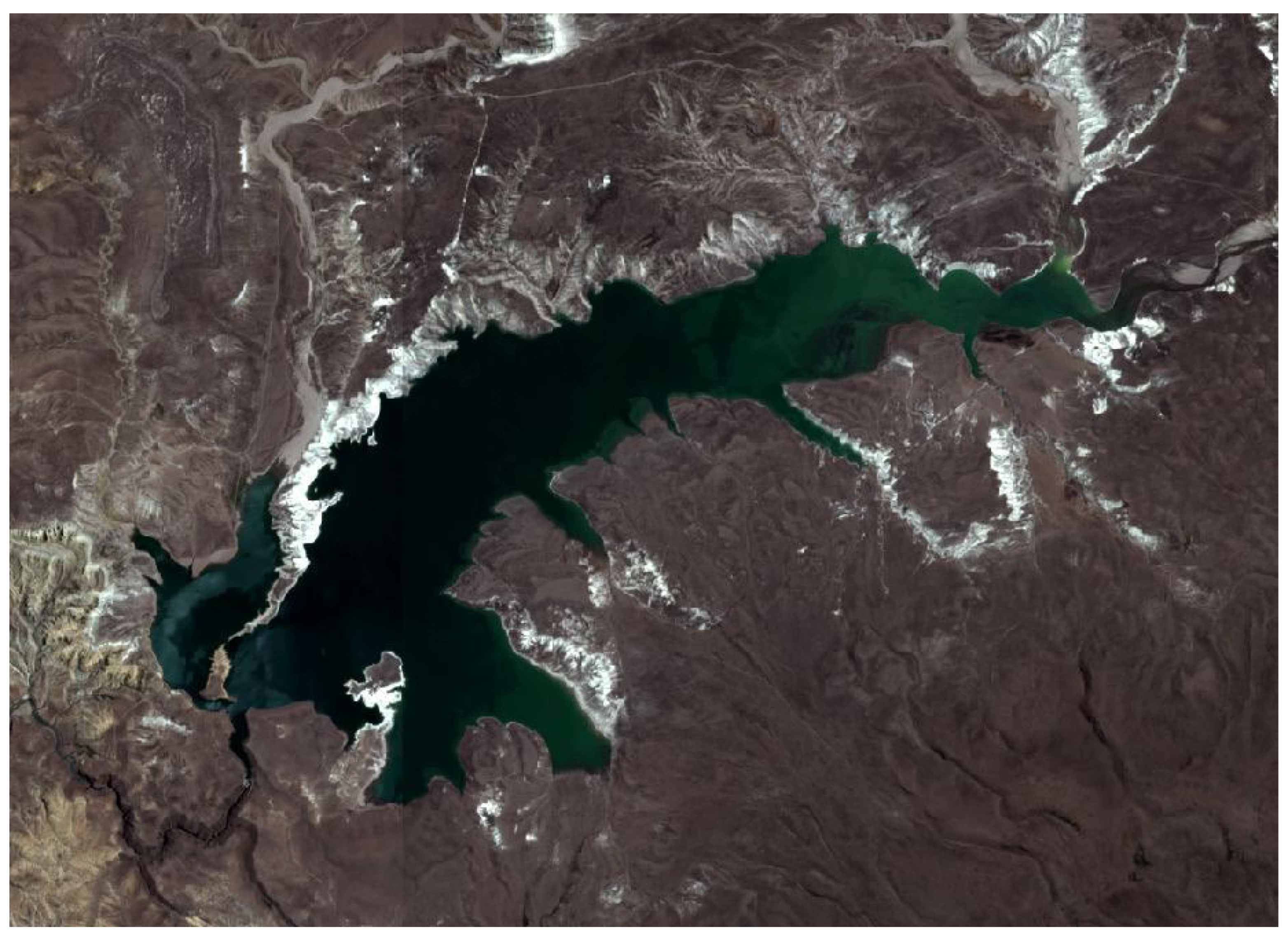
Figure 2.
Multispectral satellite image of a lake in Arequipa.
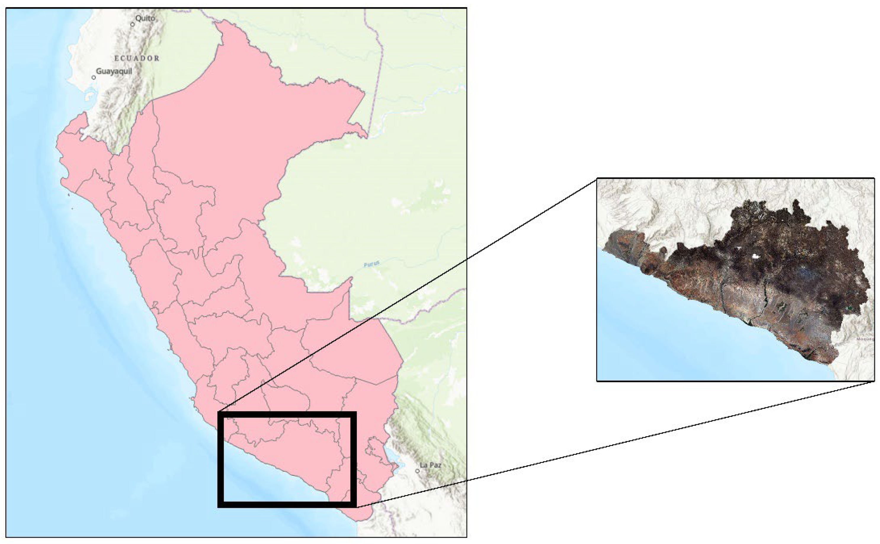
Figure 3.
Land cover classification using machine learning algorithms.
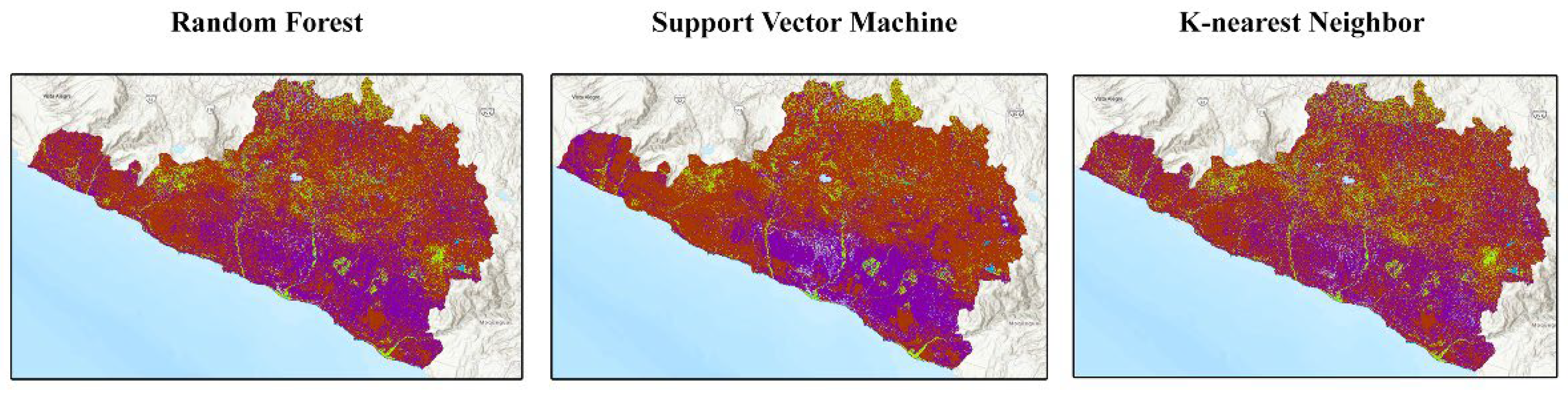
Figure 4.
Inland water bodies classification.
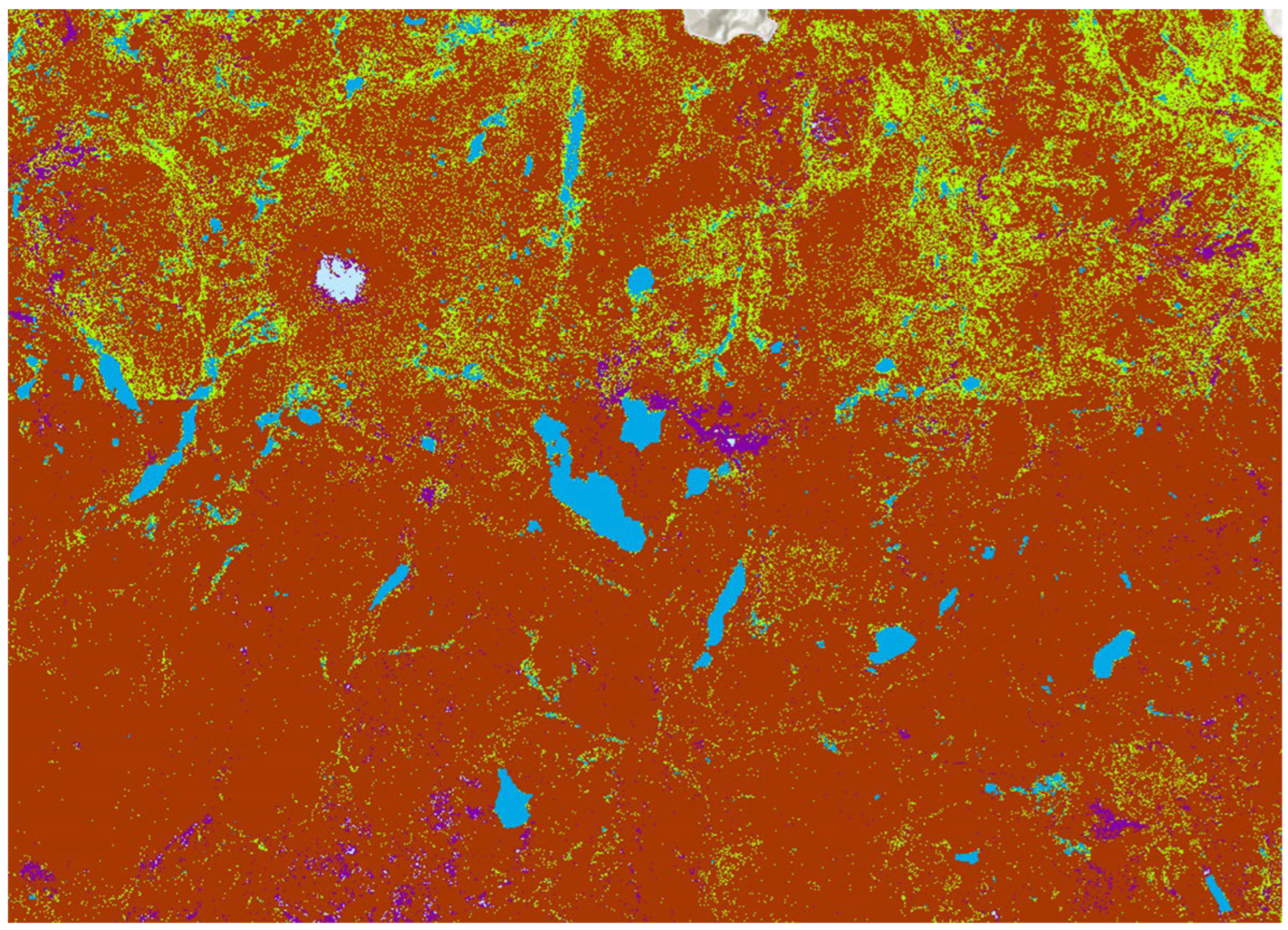
Figure 5.
Randomly generated points.
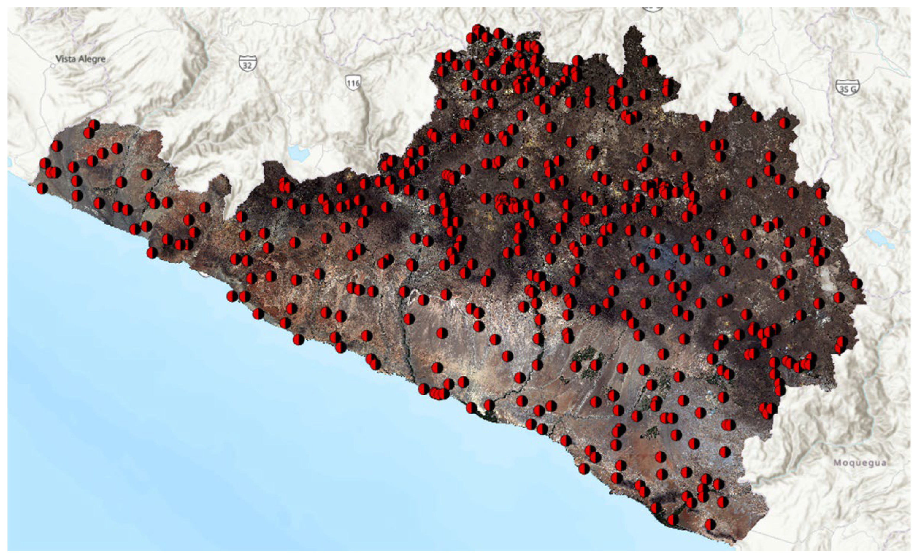
Figure 6.
Verification of precision random points.
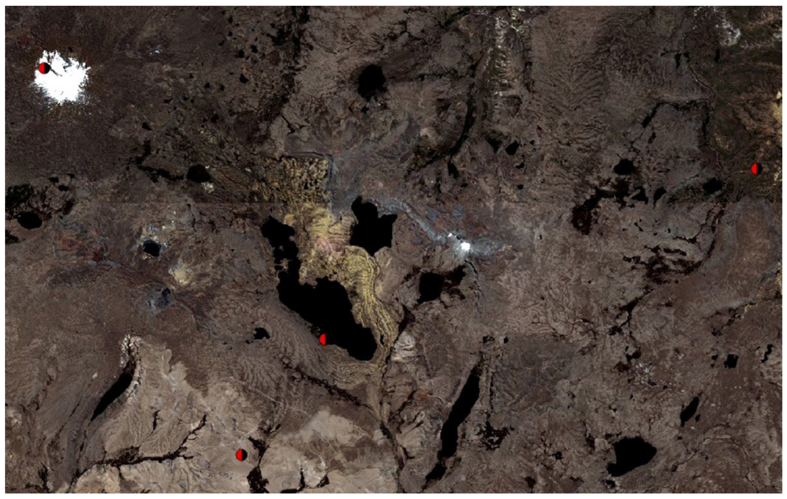

Table 1.
Work units by country.
| Country | Work units |
|---|---|
| Venezuela | 5 |
| Colombia | 35 |
| Ecuador | 11 |
| Perú | 60 |
| Bolivia | 40 |
| Argentina | 73 |
| Chile | 49 |
Table 2.
Work units corresponding to the Arequipa region.
| Work Unit | Country | Latitude | Longitude |
|---|---|---|---|
| U97 | PER | -14.1274610 | -72.553376 |
| -15.0312010 | -73.483256 | ||
| U98 | PER | -14.1274760 | -71.638882 |
| -15.0312300 | -72.568750 | ||
| U99 | PER | -14.1274550 | -70.758722 |
| -15.0312340 | -71.654846 | ||
| U100 | PER | -14.1274530 | -69.812202 |
| -15.0312290 | -70.742090 | ||
| U101 | PER | -14.1274950 | -68.893070 |
| -15.0312450 | -69.822948 | ||
| U102 | PER | -14.9998050 | -73.339385 |
| -15.9035050 | -74.269130 | ||
| U103 | PER | -15.0187220 | -72.425584 |
| -15.9224060 | -73.355411 | ||
| U104 | PER | -15.0197130 | -71.500456 |
| -15.9224070 | -72.434329 | ||
| U105 | PER | -15.0187510 | -70.580027 |
| -15.9224500 | -71.509844 | ||
| U106 | PER | -15.0187470 | -69.654652 |
| -15.9224360 | -70.584498 | ||
| U107 | PER | -15.9125520 | -69.317483 |
| -16.8161770 | -70.251337 | ||
| U108 | PER | -15.9125550 | -70.242837 |
| -16.8161780 | -71.176718 |
Table 3.
Class labelling.
| Color | Description |
|---|---|
| Water | |
| Rocky / Desert | |
| Crop | |
| Urban | |
| Ice |
Table 4.
Class-based accuracy assessments between Random Forest (RF), Support Vector Machine (SVM), and K-nearest Neighbor (KNN). The following metrics, User Accuracy (UA), Producer Accuracy (PA), Overall Accuracy (OA), and Kappa (κ), are reported for each assessment per land-cover class.
Table 4.
Class-based accuracy assessments between Random Forest (RF), Support Vector Machine (SVM), and K-nearest Neighbor (KNN). The following metrics, User Accuracy (UA), Producer Accuracy (PA), Overall Accuracy (OA), and Kappa (κ), are reported for each assessment per land-cover class.
| Random Forest | Support Vector Machine | K-nearest Neighbor | ||||
|---|---|---|---|---|---|---|
| Class | UA | PA | UA | PA | UA | PA |
| Water | 0.6456205 | 0.79353375 | 0.620482 | 0.77018375 | 0.688648 | 0.8031175 |
| Rocky/Desert | 0.97863625 | 0.30275325 | 0.975294 | 0.29107275 | 0.97 | 0.26536325 |
| Crop | 0.17207925 | 0.59821425 | 0.17261925 | 0.56818175 | 0.06799775 | 0.5694445 |
| Urban | 0.014706 | 0.25 | 0.01171875 | 0.10714275 | 0.0108695 | 0.0714285 |
| Ice | 0.44293475 | 0.75 | 0.3282895 | 0.75 | 0.23449525 | 0.73958325 |
| Overall Accuracy (OA) | 0.46457125 = 46.46% | 0.43555275 = 43.56% | 0.4091195 = 40.91% | |||
| Kappa (k) | 0.31436175 = 31.44% | 0.284222 = 28.42% | 0.24825925 = 24.83% | |||
Table 5.
Comparison of metrics between Random Forest, Support Vector Machine, and K-nearest Neighbor. The following metrics are reported for each Machine Learning algorithm: Producer Accuracy, User Accuracy Mean, Precision, Recall, Error Rate, and F1-Score.
Table 5.
Comparison of metrics between Random Forest, Support Vector Machine, and K-nearest Neighbor. The following metrics are reported for each Machine Learning algorithm: Producer Accuracy, User Accuracy Mean, Precision, Recall, Error Rate, and F1-Score.
| ML Algorithm | Producer Accuracy | User Accuracy | Accuracy Mean | Precision | Recall | Error Rate (%) | F-1 Score |
|---|---|---|---|---|---|---|---|
| Random Forest | 0.79353375 | 0.6456205 | 0.719577125 | 0.64562054 | 0.79353355 | 28.04% | 0.711976 |
| Support Vector Machine | 0.77018375 | 0.605482 | 0.687832875 | 0.62048207 | 0.77018398 | 31.22% | 0.687275 |
| K-Nearest Neighbor | 0.80311758 | 0.688648 | 0.745882788 | 0.68864796 | 0.80311772 | 25.41% | 0.741491 |
Disclaimer/Publisher’s Note: The statements, opinions and data contained in all publications are solely those of the individual author(s) and contributor(s) and not of MDPI and/or the editor(s). MDPI and/or the editor(s) disclaim responsibility for any injury to people or property resulting from any ideas, methods, instructions or products referred to in the content. |
© 2025 by the authors. Licensee MDPI, Basel, Switzerland. This article is an open access article distributed under the terms and conditions of the Creative Commons Attribution (CC BY) license (http://creativecommons.org/licenses/by/4.0/).
Copyright: This open access article is published under a Creative Commons CC BY 4.0 license, which permit the free download, distribution, and reuse, provided that the author and preprint are cited in any reuse.


