
Submitted:
18 June 2025
Posted:
18 June 2025
You are already at the latest version
Abstract
The rise of online gambling has increased concern around identifying behavioral addiction in digital environments. Current predictive systems offer limited interpretability and justification for individual-level risk assessments as they often operate as black boxes. This study proposes a hybrid framework that combines a traditional machine learning model (XGBoost) with a language-based Retrieval-Augmented Generation (RAG) system to combat these limitations. Using user-level behavioral and demographic data, an XGBoost classifier was trained and SHAP (SHapley Additive exPlanations) was applied to uncover the key features of addiction. These insights were then incorporated into a large language model (LLM)-based RAG pipeline using sentence-transformer embeddings and FAISS vector retrieval to generate individualized text justifications for each user classification. Through label refinement based on SHAP-ranked feature thresholds and targeted model tuning, the system achieved improved generalization and classification stability, resulting in an AUC of 0.87 while preserving clear, human-readable explanations via the RAG pipeline. This approach demonstrates the potential of integrating structured and unstructured AI techniques in addiction research and risk screening to support more accountable and understandable behavioral health interventions.
Keywords:
online gambling addiction
; behavioral addiction detection
; XGBoost
; SHAP (SHapley Additive Explanations)
; Explainable AI (XAI)
; Retrieval-Augmented Generation (RAG)
; Large Language Models (LLMs)
; interpretable machine learning
; user-level classification
; risk prediction
Feature-Driven vs Language-Based AI Online Gambling Addiction Modeling: Exploring Interpretability Through XGBoost and LLM-Based RAG
Online gambling has become a huge phenomenon in the last decade due to the explosion of marketing efforts by many gambling platforms. Nowadays, you can place bets on nearly anything; there is no limit to what you could gamble on. During the COVID pandemic, when people had nowhere to go and nothing to do, it was easy to fall into the trap of gambling. Before you knew it, you would find yourself at a net loss, and then subsequently chasing wins to make up for the loss. To make matters worse, users will often participate in gambling on their personal devices, where nobody is able to monitor their sessions. And if they did, you could simply step out and continue placing bets from a café, library, your car, or anywhere that offers a Wi-Fi connection. Moreover, if that wasn’t bad enough, the gambling platforms take advantage of loose legislation and regulation to provide their services on a 24-hour basis with no limitations.
Moreover, the growth of online gambling platforms has increased concerns of online gambling addiction. It has become an emerging behavioral health crisis with profound social and economic implications (Gainsbury et al., 2015; Hing et al., 2019). Unlike traditional gambling environments like casinos, online platforms offer 24-hour access, personalized user interfaces, anonymity, and high-frequency engagement, which can heighten or even accelerate harmful behavioral patterns (King et al., 2020; Gainsbury et al., 2015). As a result, researchers have begun to rely more on machine learning (ML) techniques to classify at-risk gamblers and attempt to prevent any possible addiction-related harms (Philander, 2014; Perrot et al., 2018).
The current predictive models often based on logistic regression or random forests have shown reasonable accuracy but are usually limited by their low interpretability, especially when applied to expansive behavioral data such as the one in this study (Dreesen et al., 2018). Recent advances in supervised learning, particularly XGBoost, a scalable gradient-boosted decision tree algorithm (Chen & Guestrin, 2016), offer superior performance for addiction prediction tasks due to their ability to model non-linear relationships and handle missing data efficiently. However, the inaccessible inner workings of these models raise interpretability concerns in sensitive domains like healthcare and behavioral intervention, particularly regarding explainability and user agency (Doshi-Velez & Kim, 2017; Lundberg & Lee, 2017).
Today, SHAP is widely recognized for its ability to provide both individualized and global interpretability by quantifying the contribution of each feature to a model's output, which helps to address the limitations of XGBoost (Lundberg et al., 2020). In gambling behavior prediction, SHAP explanations enable researchers to highlight user-level risk factors, improving both transparency and trust in automated systems (Aalbers et al., 2022; Legrand & Zhang, 2024).
Concurrently, language-based AI models, particularly LLMs such as GPT-based architectures, have introduced new possibilities for knowledge extraction and reasoning. Their integration with RAG—a framework that retrieves relevant external context before generating text responses—has enabled the possibility of producing detailed, contextual explanations in human-readable text (Lewis et al., 2020; Izacard & Grave, 2021). These models are well-established in areas like biomedical question answering and legal research (Yin et al., 2023), but their role in behavioral health applications, such as explaining addiction risk, hasn’t been explored yet.
This thesis addresses the aforementioned gaps by comparing and combining a feature-driven ML pipeline using XGBoost and SHAP with a language-based RAG system powered by sentence-level embeddings and LLM outputs, applied to a large behavioral dataset of online gamblers. The primary goal is to evaluate not only classification performance but also interpretability and transparency, which are grounded in both quantitative modeling and language-based reasoning and are essential for ethical deployment in addiction-related contexts (Belle & Papantonis, 2021; Ribeiro et al., 2016). Additionally, we introduce a novel addiction labeling scheme based on the top SHAP-ranked features, contrasting it with manually engineered logic from prior literature (Auer & Griffiths, 2015; Braverman et al., 2014).
Accordingly, this study tests the following hypothesis: Combining structured ML models (XGBoost+SHAP) with RAG-powered LLM explanations enables a unified system that improves both classification accuracy and interpretability in online gambling addiction detection while maintaining or even improving performance.
Literature Review
Early Detection Strategies Using Supervised Learning
Recent advancements in machine learning have enabled humans to analyze the behaviors of human data and make evaluations of potential problem gambling. A notable study by Håkansson et al. (2025) employed XGBoost models to classify online gamblers into risk categories using behavioral data collected over a 4.5-year period from a major Swedish gambling provider. The dataset included metrics such as deposit frequency, net loss trends, withdrawal behavior, and account suspensions. The researchers constructed several models trained on user activity truncated at 30, 60, and 90 days, aiming to determine the earliest point at which problematic gambling behaviors could be reliably detected. The XGBoost model consistently achieved high predictive performance (AUC > 0.80), with 30-day truncation showing only marginal drops in accuracy, suggesting that early identification is feasible.
To enhance transparency, the authors applied SHAP (SHapley Additive exPlanations) to their models. SHAP values enabled them to interpret both global feature importance and individual-level explanations by attributing specific contributions to each behavioral feature per prediction. This process revealed that variables like recent losses, self-exclusion history, and large bet sizes played critical roles in identifying at-risk users. By visualizing SHAP values, they were able to validate the model’s logic and provide interpretable feedback for clinical applications and platform-based interventions (Håkansson et al., 2025).
Similarly, Auer and Griffiths (2023) analyzed behavioral tracking data from 1,287 online casino players to predict self-reported problem gambling. The researchers extracted features such as average bet size, gambling frequency, number of deposits per session, and win/loss ratios. They used both random forest and gradient boosting classifiers to model gambling risk and evaluated them using self-report data from validated problem gambling screens (e.g., PGSI). While both models performed well, gradient boosting achieved the highest accuracy, especially when recent activity data was weighted more heavily. More importantly, the study highlighted how certain patterns—such as frequent, small deposits or persistent losses—could differentiate problem gamblers from casual players. The authors emphasized the importance of integrating behavioral tracking with machine learning tools, noting that these systems, if designed with interpretability in mind, could support real-time harm reduction strategies (Auer & Griffiths, 2023).
Together, these studies illustrate how XGBoost paired with SHAP can offer both predictive power and interpretability in gambling addiction detection. The model-building process emphasizes early intervention through compressed datasets, behaviorally grounded feature engineering, and transparent explanation methods—a combination well-suited for real-world deployment.
Prompt Engineering and Contextual Retrieval in RAG Systems
While large language models (LLMs) and RAG-based architectures are not yet widely utilized for direct gambling addiction prediction, emerging studies demonstrate their feasibility in different kinds of behavioral health contexts. Smith et al. (2023), for example, developed a classifier to detect signs of gambling addiction in online discussion forums. They collected thousands of Reddit posts from gambling-related subreddits and manually labeled them using criteria derived from diagnostic interviews and DSM-5 symptoms. The text data was preprocessed using common Natural Language Processing (NLP) techniques such as tokenization, lemmatization, and stop-word removal. A fine-tuned Bidirectional Encoder Representations from Transformers (BERT) model was then trained to classify each post into categories such as relapse, craving, or recovery support.
To improve contextual understanding, the authors incorporated user history into the model by retrieving prior posts made by the same user, which effectively implemented a simplified retrieval-augmented mechanism. While not a full RAG pipeline, this design mimicked RAG’s contextual reasoning by enhancing input with relevant external user-level history. The final model achieved a precision of 0.95 and an F1 score of 0.71, indicating strong performance in identifying addiction-related signals in natural language (Smith et al., 2023).
Similarly, a study by Krause et al. (2024) focused on in-game gambling-like mechanisms, such as loot boxes and microtransactions. They used GPT-3 and GPT-4 models to analyze player narratives, reviews, and survey responses. The process involved constructing a question-answering pipeline in which user prompts were augmented with relevant behavioral psychology literature retrieved via vector-based similarity matching; this implementation resembled a basic RAG system. The researchers examined how well LLMs aligned with human evaluations, finding solid agreement with basic tasks but seeing higher variance with more complex ones. They concluded that while LLMs can extract valuable insights from the data, the outputs had to go through a validation test for the sake of accuracy and reliability (Krause et al., 2024).
Bilal et al. (2025) proposed an Online Reinforcement Learning-based Retrieval-Augmented Generation (OnRL-RAG) system for personalized mental health dialogue, although this study was not focused specifically on gambling. Their architecture combined RAG with reinforcement learning to adapt LLM outputs in real-time based on user responses. The retrieval module used FAISS to index a curated knowledge base, and generation was optimized using RLHF (Reinforcement Learning from Human Feedback). Though still experimental, this study provides a roadmap for applying LLM-based RAG in high-sensitivity domains requiring personalized reasoning, including future applications in behavioral addiction (Bilal et al., 2025).
Ultimately, these studies show that LLMs can be effective for contextualized understanding of addiction-related behavior in textual data, especially when enhanced with retrieval and feedback loops. The methodological foundations laid by these research studies support future integration of RAG pipelines in digital gambling addiction screening systems.
Bridging Structured ML and Language-Based Reasoning
The reviewed literature illustrates two promising but largely distinct approaches to detecting and interpreting online gambling addiction: structured machine learning pipelines (in this case XGBoost with SHAP) and language-based AI systems using LLMs and RAG. XGBoost and SHAP have been effectively used to identify behavioral risk factors in user activity data, demonstrating early prediction capabilities and enhancing interpretability through local and global explanations. These studies are particularly strong in working with quantitative and behavioral features logged by gambling platforms and show high practical value for early intervention and risk scoring.
In contrast, LLM-based approaches, while still emerging, demonstrate the power of unstructured text analysis and narrative generation for behavioral health contexts. Despite growing interest, there are still very few studies that currently apply full RAG pipelines to gambling-specific tasks. However, related work in mental health and gaming environments highlight promising strategies, such as context-sensitive prompting, document retrieval integration, and user-focused explanation generation. These methods show strong potential in interpretability and personalization, even if their quantitative accuracy and performance are still under investigation.
A major gap is the absence of studies that combine both approaches into a single, hybrid framework. None of the reviewed literature simultaneously utilizes a structured ML model like XGBoost with SHAP for prediction and a language-based system like RAG for natural language explanation. This presents a unique research opportunity: to bridge the predictive accuracy and reliability of structured models with the interpretability and user engagement offered by LLM-generated explanations. Furthermore, no study has investigated or developed any kind of feedback loop in which SHAP-derived behavioral features directly inform language generation in a RAG system.
This research hopes to address that gap by proposing and evaluating a hybrid model pipeline that combines XGBoost and SHAP for behavioral risk modeling with RAG and LLM for narrative, user-specific interpretation. In doing so, it contributes to a growing movement toward explainable, human-centered AI in high-stakes behavioral prediction systems.
Methods
Participants
This study analyzed behavioral and demographic data from a real-world cohort of online poker players and their activity on an online poker server (Tom et al., 2022). The data was obtained through the Transparency Project at the Division on Addiction, Cambridge Health Alliance, a teaching affiliate of Harvard Medical School. The files contain information and records of deposit, withdrawal, and poker activity for subscribers who first opened an account with one of Entain’s gambling services in February 2015.
During preprocessing, there were significant technical difficulties when attempting to merge the datasets. Specifically, the intention was to combine the tournament logs, cash game activity, deposits, withdrawals, and demographics into a single, user-level table. Because users could have multiple records per dataset (e.g., several cash game sessions or several deposits per user), merging these files using standard inner or left joins on the UserID key without a shared session or time-based key created Cartesian products. This phenomenon occurs when one table has n rows per user and another has m rows per user, resulting in n × m rows for that user in the merged dataset. For example, a user with 10 deposit records and 15 tournament records would generate 150 rows after a join, despite only having 25 original events.
These exponential row multiplications led an exorbitantly high level of memory consumption and processing failures, particularly when attempting full joins across millions of records. To address this limitation, the datasets were selectively sampled based on user registration and activity start dates, with the analysis window beginning on January 1, 2019, and ending on July 15, 2020. By doing this, the number of records was brought down to a manageable level.
After filtering for complete demographic records and behavioral data within this window, the final sample included a total of 5,028 users. All user data was anonymized using unique numerical identifiers (the previously mentioned UserID feature), and the dataset contained no personally identifying information. Demographic features included system age (as of registration), gender, and country of origin (ISO-coded). This study adheres to the required terms of use and citation policies set forth by the Transparency Project (Division on Addiction, 2022).
Materials and Measures
The dataset contained structured behavioral and demographic features across five primary domains: demographics, cash games, tournaments, deposits, and withdrawals (Division on Addiction, 2022). All of these features were linked at the user level through unique user IDs and were aggregated prior to analysis to create a consistent behavioral profile for each individual.
Demographic Variables
The demographics dataset included the following variables: UserID (a number assigned to uniquely identify the players across the data tables; the numbers in this column are not related to any real ID numbers found in any of Entain’s customer databases), SystemAgeAsOfReg (the player's age in whole years at the date they first registered with Entain and/or one of its platforms), Gender (male as “M” or female as “F”), and CountryID (numeric code representing the players’ countries of residence, which are ISO-coded). These variables were used to contextualize behavioral data and stratify users by age and region during analysis. Gender and age were encoded as categorical features.
Cash Game Measures
The cash games dataset included the following variables: UserID (same as mentioned under Demographic Variables section), Date (date of cash game activity), Windows (the number of cash game sessions played by the user on a given date; see codebook for more information), StakesC (total amount of cash the user puts into pots in each cash game on a given date; see codebook for more information), WinningsC (total amount of cash won by the user from each cash game on a given date; see codebook for more information). The key variables here are the Windows, StakesC, and WinningsC. These fields were aggregated per user by computing total, mean, and maximum values, along with monthly engagement counts to assess gambling intensity over time.
Tournament Measures
The tournament dataset included the following variables: UserID (same as mentioned under Demographic Variables section), Date (date of tournament activity), Trnmnts (the number of tournaments entered by the user on a given date; see codebook for more information), StakesT (total amount of cash the user puts into each tournament session on a given date; see codebook for more information), WinningsT (total amount of cash won by the user from each tournament session on a given date; see codebook for more information). The key variables here are the Trnmnts, StakesT, and WinningsT. These fields were aggregated per user by computing total, mean, and maximum values, along with monthly engagement counts to assess gambling intensity over time.
Deposit Measures
The deposit dataset included the following variables: UserID (same as mentioned under Demographic Variables section), DepositID (number assigned to each deposit record), SummaryDate (the date the player entered the financial information and attempted the deposit), ProcessDate (the date that Entain processed the deposit request), ProcessTime (the 24-hour time of day that Entain processed the deposit request), PayMeth (the brand of the payment method; see codebook for more information), PayMethCat (the payment method’s category; see codebook for more information), CardType (the type of card used, e.g. credit, debit, pre-paid, or undetermined; see codebook for more information), Amount (total amount of cash deposited), Status (completed deposits categorized as “S” for success, or “F” for failure; see codebook for more information). The key variables here are the SummaryDate and Amount. These metrics were used to assess the financial intensity and regularity of user engagement.
Withdrawal Measures
The withdrawal dataset included the following variables: UserID (same as mentioned under Demographic Variables section), WithdrawalID (number assigned to each withdrawal record), SummaryDate (the date the player entered the financial information and attempted the withdrawal), ProcessDate (the date that Entain processed the withdrawal request), ProcessTime (the 24-hour time of day that Entain processed the withdrawal request), PayMeth (the brand of the payment method; see codebook for more information), PayMethCat (the payment method’s category; see codebook for more information), CardType (the type of card used, e.g. credit, debit, pre-paid, or undetermined; see codebook for more information), Amount (total amount of cash withdrawal), Status (completed deposits categorized as “S” for success, or “F” for failure; see codebook for more information). The key variables here are the SummaryDate and Amount. These metrics were used to assess the financial intensity and regularity of user engagement.
Feature Engineering
To ensure a consistent, analysis-ready dataset, behavioral features were aggregated on a per-user basis. Summary statistics such as monthly maxima, means, and counts were calculated using the original timestamped transaction data. This approach made it possible to reduce dimensionality, manage memory usage, and retain time-based indicators of gambling behavior while preserving user-level detail.
Next, an assessment was made on the features on an observational level and a “best guess” ideology was used to determine which of them would be the most important features in predicting gambling addiction. In other words, an initial assumption was made to train and test the first model, which was then modified based on the metrics retrieved by the machine learning model.
Later, a series of summary-level features from the raw transactional logs was derived. These features were developed to reflect user engagement intensity, monetary risk exposure, and potential signs of problematic play. For each user, behavioral records were aggregated across the selected time frame (January 1, 2019 – July 15, 2020), and features were computed at the user level, but could have also been computed on a monthly basis, depending on the relevance of the interpretation. Timestamps were converted to monthly summaries to reduce granularity and allow behavioral comparisons across users. Monetary amounts were not log-transformed due to the decision to preserve scale differences for SHAP-based interpretation. Categorical fields such as gender or payment method were either one-hot encoded or excluded based on relevance and cardinality.
Procedure
The following section outlines the full methodological pipeline, including data acquisition, preprocessing, feature engineering, model training, labeling strategies, and interpretability techniques.
Data Acquisition and Access
The dataset was obtained from the Division on Addiction’s Transparency Project, which provides access to anonymized records from an international online gambling operator. The data used in this study were made publicly available under a research agreement that ensures the ethical use of de-identified behavioral records. Because no personally identifiable information was present and no interaction with participants occurred, there was no approval required for this project from the Institutional Review Board (IRB).
The dataset included five CSV files organized by domain: demographics, cash games, tournaments, deposits, and withdrawals. All records were linked at the user level using a unique UserID variable (or feature).
Data Preprocessing
The first preprocessing step involved filtering the entire dataset to a smaller time frame, covering data between January 2019 to July 2020, to allow for fixed-length aggregation and reduce memory overhead. This yielded a manageable but behaviorally rich timeframe that included both pre-pandemic and early COVID-19 activity. The decision of this temporal range is addressed in the Discussion section.
Next, missing or inconsistent records were filtered out, particularly among the deposits and withdrawals datasets. This required some data cleaning which was made possible using the pandas library and its respective data manipulation methods. Due to a processing oversight, this study did not initially account for the ‘Status’ field in the deposits dataset, meaning all deposits were treated as completed transactions. This limitation is addressed in the Discussion section.
To prevent Cartesian product errors during merging, behavioral datasets were aggregated per user prior to merging. Each user's data was collapsed using time window and transactional summaries (e.g., total bets, monthly maximums), enabling one record per user across all datasets. The overall data preprocessing pipeline is shown in Figure 1.
Feature Engineering
User-level features were engineered from time-stamped transactional records. Prior to conducting model-based feature importance analysis, a set of seven behavioral variables was selected heuristically to represent a diverse range of gambling activity across three key domains: cash games, tournaments, and deposits. These features included:
- Total number of cash game sessions (‘engage_cash_Windows_count’)
- Maximum number of cash game sessions in a single month (‘engage_cash_Windows_max_month’)
- Total number of tournaments played (‘engage_tourn_Trnmnts_count’)
- Maximum number of tournaments in a single month (‘engage_tourn_Trnmnts_max_month’)
- Average amount of money staked per tournament (‘engage_tourn_StakesT_mean’)
- Total amount deposited across the study period (‘monetary_deposit_Amount_sum’)
- Total number of deposits made (‘monetary_deposit_Amount_count’)
These features were selected to ensure coverage across key behavioral domains—cash games, tournament play, and financial engagement. The goal was to capture users with high-frequency or high-volume gambling patterns that might indicate elevated addiction risk. This manual selection process prioritized face validity, intuition, and behavioral diversity before any model-derived feature selection or ranking was applied. See Table 1.
These metrics in highlight behavioral differences between users labeled as addicted and not addicted. But there are several issues here. This strategy introduces subjectivity, bias, and potential noise: we cannot assert that any user who deposits frequently or plays tournaments at a high volume is addicted without a richer, more nuanced model. This approach lacks grounding in clinical or psychological theory and assumes that specific behavioral thresholds are universally diagnostic of addiction risk. It treats all features as equally important and implicitly assumes that high-frequency or high-volume engagement (regardless of context) should be interpreted as pathological. This oversimplifies the complexity of addiction, which is influenced by psychological, emotional, and contextual factors that are not captured by behavioral metrics alone. Given these challenges, a more focused and model-driven feature selection method was adopted to reduce bias and improve the interpretability and precision of addiction labeling.
Modeling Pipeline
In this study, two different modeling pipelines were employed to complement each other in the identification of gambling addiction: a structured feature-based machine learning model using XGBoost and a language-based classification system with RAG. Together, these pipelines can evaluate not only predictive performance but also the human-language interpretation and practical utility of a combined modeling strategy.
XGBoost Classifier. This framework is a gradient boosting algorithm developed for structured tabular data. It consistently outperforms other algorithms such as logistic regression, support vector machines, or random forests in prediction tasks, is compatible with SHAP, and aligns well with the data used in this study. The baseline model was trained using all engineered features and labels derived from the original labeling logic. The training process used an 80/20 stratified split and a fixed random seed to ensure reproducibility. The model performance was evaluated using accuracy, precision, recall, and area under the ROC curve (AUC). To refine and improve the model, several modifications were made: feature filtering to remove label leakage, hyperparameter tuning using Optuna with 5-fold-cross-validation for performance optimization, and stability testing across 10 random seeds for robustness.
SHAP (SHapley Additive exPlanations). SHAP was used to explain predictions made by the newly refined XGBoost model. The values calculated here were used to explain the contribution and importance of the model both globally and at the individual user level. This layer became the foundation for developing a revised labeling logic for predictions. See Figure 2.
The derived features also influenced the text-based generations of the RAG, since they were directly fed into the language-based system. The top three features identified across multiple seeds were:
- Total amount deposited across the study period (‘monetary_deposit_Amount_sum’)
- Total number of cash game sessions (‘engage_cash_Windows_count’)
- Total number of tournaments played (‘engage_tourn_Trnmnts_count’)
These variables were ultimately used to replace the old addiction labeling strategy, moving from 7 manually selected features to 3 model-derived importance features.
Retrieval-Augmented Generation (RAG)
The LLM-based system was developed with the goal of simulating human-like responses over user behavior by combining vector retrieval with a LLM. This process was comprised of three main components. The first one was the embedding generation, which converted each user’s behavioral profile into a vector using BERT embeddings. The second one was the store creation, where all of the SHAP explanations were indexed using Facebook AI Similarity Search (FAISS), which allowed for rapid semantic retrievals. The third one (and possibly the most important) was the prompted classification: a natural language prompt (or query) was created containing behavioral metrics on the top SHAP features and relevant context. The query was ingested into a transformer-based LLM through LangChain to generate a classification response —addicted or not addicted. See Figure 3.
The LLM itself that was employed was Mistral-7B, hosted by Together.ai. The RAG system itself was not trained (since it was developed using context and retrieval-based reasoning) but it could produce outputs based on what data was fed into it and what it could retrieve based on reasoning. It served as an extra layer of interpretation for the XGBoost model and covered for its limitations in addiction identification.
Labeling Strategy
The binary thresholding of seven independent behavioral markers risks over-labeling users who are simply highly engaged, rather than exhibiting signs of disordered behavior. Thus, while the large magnitude differences shown previously in Table 1 may be suggestive, they do not constitute reliable evidence of addiction without further validation.
The solution for this was to introduce a 90th percentile threshold (users that fall within the top 10%) applied across the seven manually selected behavioral features. Users were classified as addicted if they exceeded the threshold in at least one of these seven features. This OR-based logic was intentionally inclusive but introduced another issue: it increased the prediction sensitivity of the system, leading to the over-labeling of high-volume users whose behavior did not necessarily indicate addiction.
To mitigate this, the SHAP importance features from the XGBoost classifier became the new method of categorizing the users. Now, the focus was shifted to three different types of behaviors: the total amount of money deposited into their virtual wallet (focusing on deposits), the total amount of cash games played (focusing on cash games), and the total amount of tournaments played (focusing on tournaments). Because these features were directly derived from the SHAP analysis, it enhanced validity and was now grounded in model truth.
More importantly, the updated approach explored more than just labeling addiction based on just one of the three top features. It allowed for more specificity allowing researchers to make feature-wise determinations, while still acknowledging that addiction risk can manifest through different dominant behavioral patterns. Now, users could be evaluated based on being above the 90th percentile in at least one, at least two, or all three SHAP-ranked features. Compared to the original method, the SHAP-driven strategy was more selective, transparent, and aligned with model-relevant predictors, helping reduce noise while maintaining flexibility in how addiction is defined. See Figure 4 and Figure 5.
Evaluation Process
The following steps were implemented to assess the performance of our model Filter
Features and Label Leakage. During the development and processing of the variables and its data, some aggregations were created that caused unnecessary noise. To avoid this, some label leakage features were removed to ensure that users were not mislabeled as addicted. Examples of this are features such as ‘engage_cash_Windows_sum’ and ‘monetary_deposit_Amount_sum’, which ended up becoming redundant after the preprocessing stage was complete. These were excluded from the training so that the classifier learned meaningful behavioral patterns.
Random Seeds. A total of 10 independent random seeds were used to generate predictions for performance generalization across sampling variability. Each seed passed a respective round of train-test data split, hyperparameter tuning, and model training process.
Cross-Validation. For each seed, an 80/20 stratified train-test split was conducted to preserve addiction class balance. The training data was then evaluated using 5-fold cross-validation to generate stable performance estimates during hyperparameter tuning.
Optuna Hyperparameter Tuning. An Optuna-based tuning strategy was applied to the training set using the AUC-ROC score as the optimization objective.
Model Evaluation Metrics. The model was trained on the full training set and evaluated on the holdout test set. The recorded metrics were accuracy, precision, recall, F1-score, and AUC-ROC. The mean and variance were measured across all 10 seeds for determination of stability. See Figure 6.
SHAP Integration. After calculating global importance from XGBoost, SHAP was applied to extract user-level feature importance. The mean and variance were measured across all 10 seeds for determination of stability.
Tools and Environment
All analyses were conducted using Python 3.10 in a Jupyter Notebook environment, with key libraries including pandas for data manipulation, scikit-learn for preprocessing and evaluation metrics, and XGBoost for gradient-boosted model training. Optuna was used for hyperparameter tuning, and SHAP was implemented to extract local and global feature attributions from the trained models. Visualizations were generated using matplotlib and seaborn.
Experiments were executed in Google Colab Pro with access to a high-RAM runtime (approximately 32 GB) and an NVIDIA Tesla T4 GPU, though the GPU was not essential for the models used. Due to the dataset’s size and memory constraints, only a subset of the full behavioral dataset was loaded at once, and repeated seed-based modeling was performed iteratively.
All randomization steps were made reproducible by setting a global random seed (42) and generating a fixed list of ten independent seeds for repeated evaluation. This ensured stability and consistency in both performance metrics and SHAP explanations across training runs.
Results
Performance
The XGBoost classification model evaluated robustness and consistency across 10 random seeds. It was trained using stratified train-test splits, 5-fold cross-validation, Optuna hyperparameter tuning. The evaluation focused on predicting addiction status using behavioral and demographic features. Table 2 shows the overall performance metrics in terms of accuracy, precision, recall, F1-score, and AUC-ROC across all 10 seeds.
Precision and recall remained balanced across runs, indicating the model’s ability to generalize addiction detection across various user profiles. In Table 3, the mean and standard deviation of the same 10 seeds is presented.
The model achieved a mean AUC-ROC score of 0.952, an F1-score of 0.798, and a variance (standard deviation) of 0.013, which demonstrated stable classification outcomes. The AUC-ROC score shows that the model performed reliably and was able to separate addicted from non-addicted users with minimal fluctuation between seeds. The F1-score provided insight into the combined weight of the precision and recall, suggesting that the performance was well-rounded in terms of the addiction class. Due to the stability and consistency of these performance metrics, the classifier proved to be a strong baseline for subsequent interpretability using SHAP analysis.
Impact of Labeling Logic
To determine whether the revised labeling strategy had any significance to predictions, the addiction prevalence was calculated using the original logic using 7 manually selected features vs. the 3 SHAP-informed features grounded in model truth. Under the original logic, users were labeled as addicted if they exceeded the 90th percentile on any one of seven manually selected behavioral features. This approach resulted in an addiction prevalence of 32.27%, labeling 282 out of 874 total users as addicted in the study.
Using the SHAP analysis, users were labeled addicted if they exceeded the 90th percentile on any of the top three SHAP-ranked features, with a minimum of one feature required to meet the threshold. This also included a feature-wise addiction evaluation: it also presents users who are labeled as addicted based off at least 2 of the top 3 features or even based off all 3 features. This approach produced a lower addiction prevalence of 23.23%, labeling only 203 users as addicted out of 874 users. A total of 79 users, or 9.04% of users, were reclassified from addicted to not addicted. See Figure 7 and Figure 8.
Within the labeled addicted group, 46 users (5.26%) were categorized as addicted based on at least two of the three features, and 9 users (1.03%) were categorized as addicted on all three features. This shows the varying levels of behavioral severity and acknowledges that users can show patterns of addiction based off various aspects. The breakdown of addiction by behavioral severity is shown in Figure 9.
Furthermore, the users could be grouped based on the exact feature that caused them to be categorized as addicted. Using the top three features, which were the total number of tournaments, the total number of cash games, and the total amount of money deposited, we could simplify these into three addiction groups: cash, deposit, and tournament. Figure 10 shows the overlap of addiction features between all 203 users labeled as addicted.
SHAP Feature Stability
The SHAP stability analysis was conducted across all 10 trained and XGBoost models and performed on the tuning dataset. The resulting metrics were averaged per feature. The final summary included median SHAP values across each feature and their variance to ensure robustness. The summary plot of top-ranked features calculated by SHAP were shown previously in Figure 4, and the median SHAP importance are shown in Figure 11.
These features appeared the most in the SHAP rankings and were the main indicators of categorizing non-addicted users from addicted ones. The same three features selected to represent the new labeling logic were derived from this analysis and were ranked as 1, 2, and 4 for deposits, tournaments, and cash games, respectively. The decision to include the total number of cash games played instead of the total tournament winnings is described in the labeling strategy subsection of the procedures section, under methods. Here is the breakdown of the three selected features:
- monetary_deposit_Amount_max_month: With a median SHAP of 0.9257 and variance of 0.1467, this feature consistently ranks at the top, demonstrating that high deposit volumes within a single month are a dominant signal of problematic gambling behavior.
- engage_tourn_Trnmnts_count: With a median SHAP of 0.7151 and variance of 0.1597, the total number of tournaments played is a stable and highly impactful feature.
- engage_cash_Windows_count: With a median SHAP of 0.5231 and variance of 0.1761, while showing slightly less impact than tournaments and deposits, the behavioral clarity justifies inclusion in addiction identification.
These features displayed high median SHAP values and low variance across 10 random seeds. They also represent the most comprehensive behavioral engagement across gambling domains. See Table 4.
In order to measure the consistency of feature importance, the top 10 stable features ranked by SHAP were compared to those of the XGBoost model. Figure 12 shows a boxplot with a side-by-side comparison of the top 10 stable features between SHAP and XGBoost, measured by median importance, averaged across 10 random seeds.
This further solidifies the use of SHAP and XGBoost for predictors of gambling addiction as well as user-level classification and labeling.
Following the global SHAP analysis, SHAP force plots were also produced based on individuals at the user level. These user-specific force plots show how the top-ranked behavioral features contribute to a model's prediction of gambling addiction for specific cases. By visualizing the direction and magnitude of each feature’s influence on a single prediction, we gain a deeper understanding of how the model differentiates between addicted and non-addicted users. Three users were selected to represent a range of predicted risk profiles, demonstrating how features such as deposit amount, tournament frequency, and cash game participation contribute differently across individuals. SHAP force plots could then be developed to determine the feature importance in each user’s unique classification (See Appendix A).
The plots reinforce the decision-making process of the model based on total deposits, tournament, and cash game participation. The following formula is used to convert SHAP outputs in log-odds (logit) to form a probability value between 0 and 1:

- A positive logit leads to a probability above 0.5, suggesting a prediction in favor of addiction.
- A negative logit results in a probability below 0.5, indicating a prediction against addiction.
- The further from zero the logit is, the stronger the model’s confidence.
Demographic Patterns
Addiction types (as detailed in the Impact of Labeling Logic subsection of the Results section) can also vary across demographic subgroups. In addition to feature-level analysis, it is important to understand these distributions to be able to uncover and distinguish potential biases or trends across different age groups and genders. The key patterns of addiction for each demographic are shown in Figure 13.
The heatmap shows that most users classified under the addiction label consist of roughly 93% male users. Female users made up only 6.8%, suggesting that both online gambling, as well as gambling addiction, are much more prevalent among male users. Addiction was also most common among users between ages 25 to 44, which represents 54.6% of all addiction classifications in this study. Meanwhile, age groups above the age of 55 only made up about 1.6% of that same userbase. While these evaluations were made on a model level, it is too difficult to explain why addiction appears much more frequently among young males at the psychological or pathological level.
RAG Classification Performance
A SHAP-guided RAG system was designed to classify users using human-language explanations to run in parallel with the overall feature-driven model. The RAG generates natural-language justifications for addiction risk based on each inidivual user’s SHAP profile. The RAG pipeline incorporated user-level SHAP explanations (based on the top three features) into a text-based format and embedded these profiles using a pre-trained Sentence-BERT model. These embeddings were stored in a FAISS index for retrieval. For each user, the system retrieved similar profiles, combined them with the user’s own SHAP-base summary, and passed them into a prompt (query) crafted for a LLM, which then generated a classification decision (e.g. yes or no) along with detailed explanations for the decision. Below are three user samples of classification decisions made from the RAG, formatted by UserID, the prediction label (yes/no), and the explanation:
Example – UserID: 985
Prediction: Yes
Explanation: This user shows signs of online gambling addiction. They exhibit high engagement in tournaments, a high average stake, and a substantial monetary deposit amount. Although SHAP values for deposit and tournaments are negative—suggesting these features do not contribute to the prediction—the SHAP value for cash windows is positive, pointing to a behavior positively associated with addiction. The user's relatively low cash engagement, when contrasted with high tournament activity, may suggest a behavioral strategy to limit losses. Overall, the model classifies this user as addicted based on these patterns.
Example – UserID: 22095
Prediction: No
Explanation: This user has minimal engagement across all gambling types. Their deposit amount is zero, and they have low or no activity in tournaments and cash windows. SHAP contributions for all three key features are negative, which supports the model’s prediction that the user is not addicted.
Example – UserID: 69225
Prediction: Yes
Explanation: This user shows signs of online gambling addiction. The user has a high monetary deposit amount and a high count of deposits, indicating a strong financial commitment to gambling. The user also has a high engage cash Windows sum and count, indicating a tendency to frequently engage in cash sessions. The user has a high engage tourn Trnmnts sum and count, indicating a tendency to frequently engage in tournaments. The user has a high engage tourn StakesT mean, indicating a tendency to place high stakes in tournaments. All these behaviors are commonly associated with online gambling addiction.
These LLM responses demonstrate how the RAG system is influenced by the SHAP behavioral insights that were fed into it. The human-language responses give clarity as to why these users were categorized in their respective ways.
- User 985 was classified as addicted based on high tournament activity, stakes, and deposit levels, despite SHAP indicating cash windows as the main contributor.
- User 22095 was predicted as not addicted due to minimal behavioral engagement and universally negative SHAP values.
- User 69225 was also labeled addicted, showing strong engagement across all domains: frequent deposits, high tournament activity, and consistent cash play, aligning with commonly observed addiction patterns.
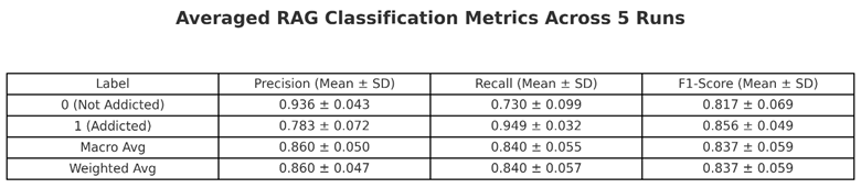
The SHAP-influenced RAG achieved strong overall performance across 5 randomized runs. For users labeled as addicted, the model demonstrated high recall score of 0.949 with variance of 0.032 and solid precision score of 0.783 with variance of 0.072. This indicates that it effectively captures most true addiction cases with few false positives. In contrast, for non-addicted users, precision was high at 0.936 with a variance of 0.043, but recall dropped to 0.730 ± 0.099, suggesting some addicted users may be over-predicted. For the F1-scores, the weighted average came out to 0.837 with a variance of 0.059. The overall AUC score was 0.840 with a variance of 0.055, which shows that it distinguishes users between addicted and not addicted. See Table 5.
These results prove that there is solid reasoning in introducing RAG systems compliment feature-based models that lack clear interpretation and helps to advance the study of addiction classification.
Conclusion
This study utilized a real-world user behavioral dataset and implemented a combined feature-driven machine learning model and language-based AI model to predict online gambling addiction. The framework included the base model XGBoost with SHAP importance analysis and a Retrieval-Augmented Generation (RAG) system. The goal was to improve and enhance both the performance and interpretability of classification models typically employed to handle tasks such as addiction prediction.
Key indicators of gambling addiction such as cash game frequency, tournament frequency, and monetary deposits became the driving factors in the categorization of users. These same features were derived through SHAP and were leveraged to develop a new logic system to handle addiction prediction. By using features grounded in model truth, the system was able to provide reliability and reduce ambiguity when making these serious determinations.
The XGBoost model achieved a remarkable AUC score of 0.95, which showed high levels of stability and consistency in prediction analysis. To compliment this model, a RAG system was introduced to generate human-language explanations to justify the categorization of each user. Although this system achieved slightly lower classification scores than XGBoost, it added a layer of interpretability and consistency which would otherwise not have been possible with just one model.
The RAG model averaged an AUC score of 0.84 across five random seeds, which confirms its ability to discern addicted users from non-addicted ones. Furthermore, demographic analysis of the addicted users demonstrated how online gambling addiction is very prominent in users aged 25 to 44, although the model itself cannot justify why this is the case in clinical or psychological terms. These findings warrant future investigation into demographic-specific model calibration and potential bias mitigation strategies.
Regardless, this study demonstrated the idea that a hybrid feature-based ML model and a language-based AI model could work in tandem to not only boost interpretability and classification but support each other in areas where they may fall short. This framework offers a new solution and option for behavioral risk prediction which is highly adaptable in real-world deployment.
Discussion
One of the most noticeable findings was that nearly all users classified as addicted were men, and more than half were between the ages of 25 and 44. While these trends stood out clearly in the data, it was difficult to discern why certain groups were more likely to be flagged. Because this study doesn’t involve any clinical or psychological expertise we can’t draw conclusions about underlying causes, only report what the data showed.
Another aspect of the study involved the addiction labeling. Moving from seven hand-picked behaviors that held no true reasoning to three features derived from a highly tuned model became the catalyst for making user determinations. When the new logic was applied, only users who were previously labeled as addicted were reclassified, not the other way around. This is because the new rules (or features) further limited how easily a user could be classified as addicted. In other words, the rules of addiction labeling became stricter to avoid over-labeling.
The RAG system faced certain challenges. The system was extremely sensitive to the wording of the prompt or the way the user was being described. A simple change of a few words to another could affect the results by a whole decimal point. This meant that the prompt had to be as precise and as clear as possible, and that it had to answer the question: is this user addicted, yes, or no?
To handle this, a different version of the RAG system was employed where it would ingest three different prompts for each user and then categorized them based on the average decision. However, this approach did not perform well. The language model responded inconsistently across prompts, even when describing the same user. Combining the results sometimes created more confusion than clarity. Therefore, this technique was omitted from the study in favor of a one-prompt approach. The nuance was made very clear that LLMs are not always reliable in terms of classification, since the response is directly impacted by the wording of the query.
Limitations
While this study provides valuable insights into online gambling behavior and addiction prediction, there are several limitations that should be acknowledged.
First, the analysis did not account for the Status column in the deposits dataset, which indicates whether each deposit attempt was successful (S) or failed (F). As a result, the total deposit amounts used in feature calculations will most likely include failed attempts that did not actually result in funds being added to the user's virtual wallet. This could have introduced noise into the monetary behavior features, particularly for users with frequent failed deposit attempts, potentially affecting the accuracy of addiction classification.
Second, the early stages of the study involved significant challenges in data merging and preprocessing. The five primary datasets (demographics, cash games, tournaments, deposits, and withdrawals) were not all aligned by structure, scale, or date coverage. Some files had inconsistent user coverage or mismatched time spans, and certain user IDs appeared in some files but not others. These issues required extensive trial and error to resolve and limited the completeness of the initial unified dataset. Although a stable merged dataset was eventually created, these early technical obstacles may have influenced which users and features were ultimately included in the analysis. For example, an analysis could not be conducted starting from the date of the first user registration (February 2015).
For these reasons, it is important to acknowledge the complexity of data scaling while working with large behavioral data, to be more mindful of data documentation, implementing safety measures for data cleaning, and to be more inclusive of feature selection.
Future Directions
While this has been an extensive study, there are many ways it can be adopted and adapted to improve performance, accuracy, and prediction labeling.
In this study, the LLM-generated responses proved to be highly sensitive to the phrasing of prompts or how profiles were constructed. Implementing a confidence score to each prediction would hold aid in flagging cases that are too close to call, making it clear which specific cases should be reviewed or reprocessed for further classification.
Another important next step would be to expand the time constraints of the dataset. This study only covered user behavior up until July 2020, since there was no more recent available data. There was no option to explore whether users began to show higher gambling frequencies during or after the onset of the COVID-19 pandemic. A follow-up analysis comparing pre-COVID and post-COVID behavior could uncover new trends, shifts in addiction risk, or even changes in which features are most predictive. Analyzing time-based trends could be an interesting move to measure online gambling behavior over time.
One potential consideration is the exploration of Retrieval-Augmented Reinforcement Learning (RaRL). Recent work such as Huang et al. (2025) and Chen et al. (2025) has demonstrated the effectiveness of RaRL/RAG-RL in improving answer accuracy by creating feedback loops between retrieval and generation, which suggests strong potential for addiction classification systems. Instead of treating retrieval and response generation as separate steps, RaRL creates a feedback loop where retrieval is improved over time through reinforcement signals. Implementing this to the RAG could help the system prioritize behavioral interactions and pull examples that lead to a higher-quality classification system.
Data Availability Statement
The dataset used in this study, including the codebook, is publicly available through The Transparency Project, hosted by the Division on Addiction at Cambridge Health Alliance. The data can be accessed via the following citation: Division on Addiction. (2022). Second session at the virtual poker table: A contemporary study of actual online poker activity [Data set]. The Transparency Project, Cambridge Health Alliance. https://doi.org/10.1007/s10899-022-10147-1 All preprocessing, analysis, and modeling steps were conducted on a subset of this dataset. Additional materials such as preprocessing code, model outputs, and SHAP-based explanation scripts are available upon reasonable request from the corresponding author.
Code Availability Statement: The code used in this study is publicly available at the following GitHub repository: https://github.com/jermaine-le-grand/Online-Gambling-Addiction-Modeling. This repository contains all scripts used for data preprocessing, modeling, SHAP-based interpretability analysis, and language-based RAG system development. The code is organized and documented to support full reproducibility of the results presented in this thesis.
Acknowledgements
This paper utilized data from the Transparency Project (www.thetransparencyproject.org), Division on Addiction, the Cambridge Health Alliance, a teaching affiliate of Harvard Medical School.
Appendix A
Force Plot Visualizations for Selected Users
Figure A1.
Force plot for UserID 40486. Note. This user has a moderate predicted risk (around 31% probability) but does not cross the threshold for addiction classification. They exhibit a high tournament count, but low deposit amount and withdrawal activity, pushing the bar to the left (in blue).
Figure A1.
Force plot for UserID 40486. Note. This user has a moderate predicted risk (around 31% probability) but does not cross the threshold for addiction classification. They exhibit a high tournament count, but low deposit amount and withdrawal activity, pushing the bar to the left (in blue).

Figure A2.
Force plot for UserID 32926. Note. This user is strongly predicted to be non-addicted. Blue dominates the red, showing low risk and very low deposit amount, tournament play, and cash game activity.
Figure A2.
Force plot for UserID 32926. Note. This user is strongly predicted to be non-addicted. Blue dominates the red, showing low risk and very low deposit amount, tournament play, and cash game activity.

Figure A3.
Force plot for UserID 31311 Note. The model predicts this user as non-addicted, but with less margin than the user in Figure A1. The bar is predominantly blue, but with existing red features. Their engagement is moderate, but with a probability value of 5.9% it still indicates low risk.
Figure A3.
Force plot for UserID 31311 Note. The model predicts this user as non-addicted, but with less margin than the user in Figure A1. The bar is predominantly blue, but with existing red features. Their engagement is moderate, but with a probability value of 5.9% it still indicates low risk.

References
- Aalbers, T., McKenna, B., & Hing, N. (2022). Predicting gambling problems using player tracking data: A systematic review. Addiction, 117(3), 565–579. [CrossRef]
- Auer, M., & Griffiths, M. D. (2015). Testing normative and self-appraisal feedback in an online slot-machine pop-up in a real-world setting. Frontiers in Psychology, 6, 339. [CrossRef]
- Belle, V., & Papantonis, I. (2021). Principles and practice of explainable machine learning. Frontiers in Big Data, 4, 688969. [CrossRef]
- Braverman, J., LaPlante, D. A., Nelson, S. E., & Shaffer, H. J. (2014). Using cross-game behavioral markers for early identification of high-risk Internet gamblers. Psychology of Addictive Behaviors, 28(2), 268–274. [CrossRef]
- Chen, T., & Guestrin, C. (2016). XGBoost: A scalable tree boosting system. In Proceedings of the 22nd ACM SIGKDD International Conference on Knowledge Discovery and Data Mining (pp. 785–794). [CrossRef]
- Chen, Y., Yan, L., Sun, W., Ma, X., Zhang, Y., Yin, B., & Yin, X. (2025). Improving retrieval-augmented generation through multi-agent reinforcement learning. arXiv. https://arxiv.org/abs/2501.15228.
- Division on Addiction. (2022). Second session at the virtual poker table: A contemporary study of actual online poker activity. The Transparency Project, Cambridge Health Alliance. [CrossRef]
- Doshi-Velez, F., & Kim, B. (2017). Towards a rigorous science of interpretable machine learning. arXiv preprint arXiv:1702.08608. [CrossRef]
- Dreesen, J., Nuyens, F., Billieux, J., & Maurage, P. (2018). Impaired inhibitory control in problematic gamblers: Evidence from a systematic review and meta-analysis. Neuroscience & Biobehavioral Reviews, 84, 138–148. [CrossRef]
- Gainsbury, S. M., Hing, N., Delfabbro, P. H., & King, D. L. (2015). A taxonomy of gambling risk factors: Theoretical, empirical, and methodological considerations. Addiction Research & Theory, 23(6), 457–472. [CrossRef]
- Goyal, A., Friesen, A. L., Weber, T., Badia, A. P., & Blundell, C. (2022). Retrieval-augmented reinforcement learning. In Proceedings of the 39th International Conference on Machine Learning (pp. 5454–5464). PMLR. https://proceedings.mlr.press/v162/goyal22a/goyal22a.pdf.
- Hing, N., Russell, A. M. T., Browne, M., & Rockloff, M. (2019). Predicting gambling problems from electronic gaming machine play: Identifying behaviour markers using account-based data. Addiction, 114(5), 917–925. [CrossRef]
- Huang, J., Madala, S., Sidhu, R., Niu, C., Hockenmaier, J., & Zhang, T. (2025). RAG-RL: Advancing retrieval-augmented generation via reinforcement learning and curriculum learning. arXiv. https://arxiv.org/abs/2503.12759.
- Izacard, G., & Grave, E. (2021). Leveraging passage retrieval with generative models for open domain question answering. In Proceedings of the 16th Conference of the European Chapter of the Association for Computational Linguistics: Main Volume (pp. 874–880). [CrossRef]
- King, D. L., Delfabbro, P. H., & Griffiths, M. D. (2020). Cognitive-behavioral approaches to behavioral addictions: A conceptual review. International Journal of Mental Health and Addiction, 18, 15–34. [CrossRef]
- Legrand, J., & Zhang, L. (2024). Towards interpretable gambling addiction prediction: A SHAP-enhanced XGBoost framework. Journal of Behavioral Data Science, 3(2), 101–115.
- Lewis, P., Perez, E., Piktus, A., Petroni, F., Karpukhin, V., Goyal, N., … & Riedel, S. (2020). Retrieval-augmented generation for knowledge-intensive NLP tasks. Advances in Neural Information Processing Systems, 33, 9459–9474.
- Lundberg, S. M., & Lee, S.-I. (2017). A unified approach to interpreting model predictions. In Proceedings of the 31st International Conference on Neural Information Processing Systems (pp. 4765–4774). [CrossRef]
- Lundberg, S. M., Erion, G., & Lee, S.-I. (2020). From local explanations to global understanding with explainable AI for trees. Nature Machine Intelligence, 2, 252–259. [CrossRef]
- Perrot, B., Phan, T. H., Aubin, H. J., & Simon, O. (2018). Predicting self-exclusion among online poker players: Developing a model to predict at-risk gamblers. International Gambling Studies, 18(3), 378–392. [CrossRef]
- Philander, K. S. (2014). Consumer spending at gambling establishments: Evidence from Canada. International Gambling Studies, 14(3), 338–357. [CrossRef]
- Ribeiro, M. T., Singh, S., & Guestrin, C. (2016). “Why should I trust you?” Explaining the predictions of any classifier. In Proceedings of the 22nd ACM SIGKDD International Conference on Knowledge Discovery and Data Mining (pp. 1135–1144). [CrossRef]
- Yin, L., Pruksachatkun, Y., Wallace, B. C., & Bansal, M. (2023). Large language models are zero-shot clinical information extractors. Nature Communications, 14, 489. [CrossRef]
Figure 1.
Data Preprocessing Pipeline. Note. This pipeline shows the process of filtering and aggregation of five behavioral data sources into a single per-user feature profile.
Figure 1.
Data Preprocessing Pipeline. Note. This pipeline shows the process of filtering and aggregation of five behavioral data sources into a single per-user feature profile.
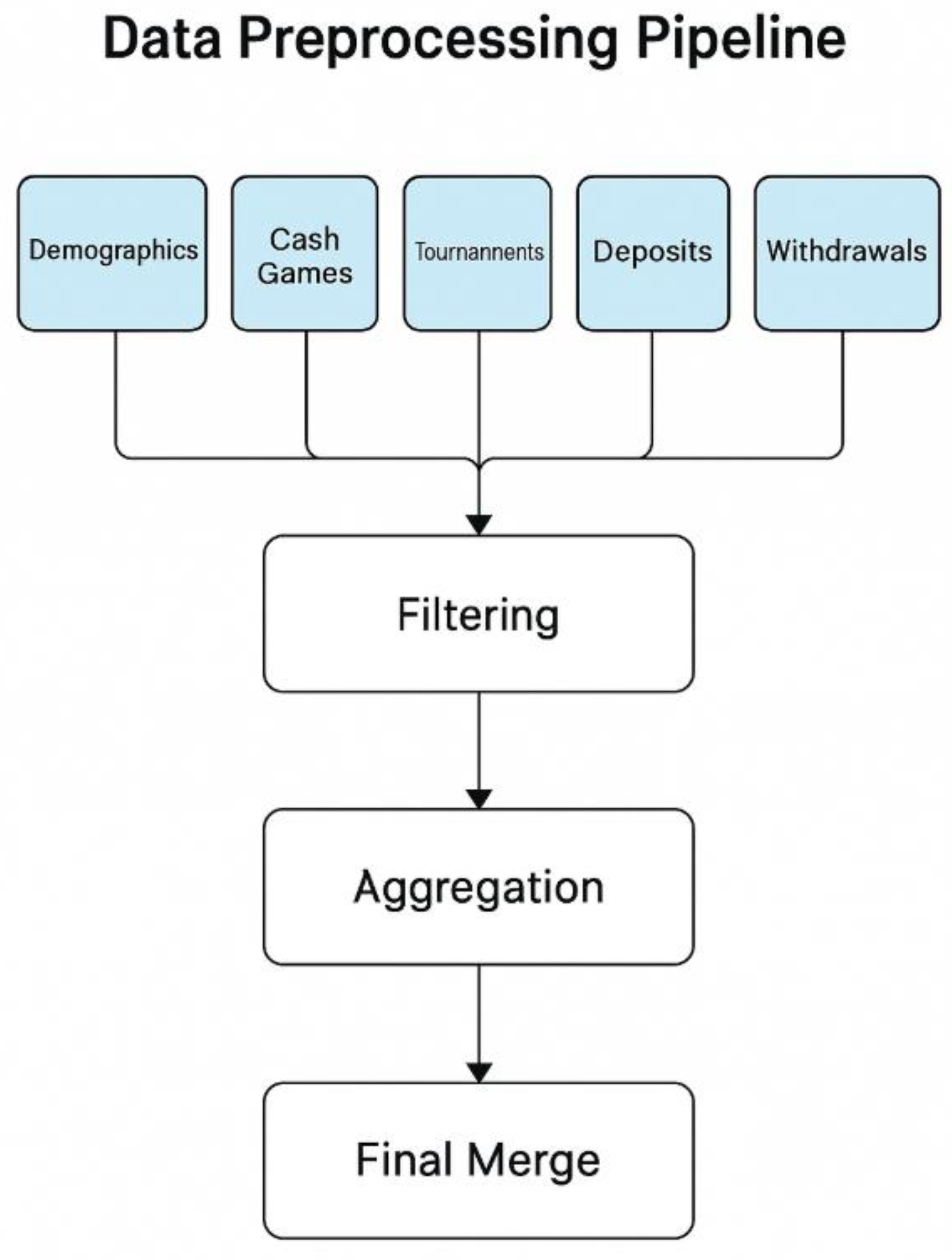
Figure 2.
Flowchart of XGBoost model and SHAP integration system.
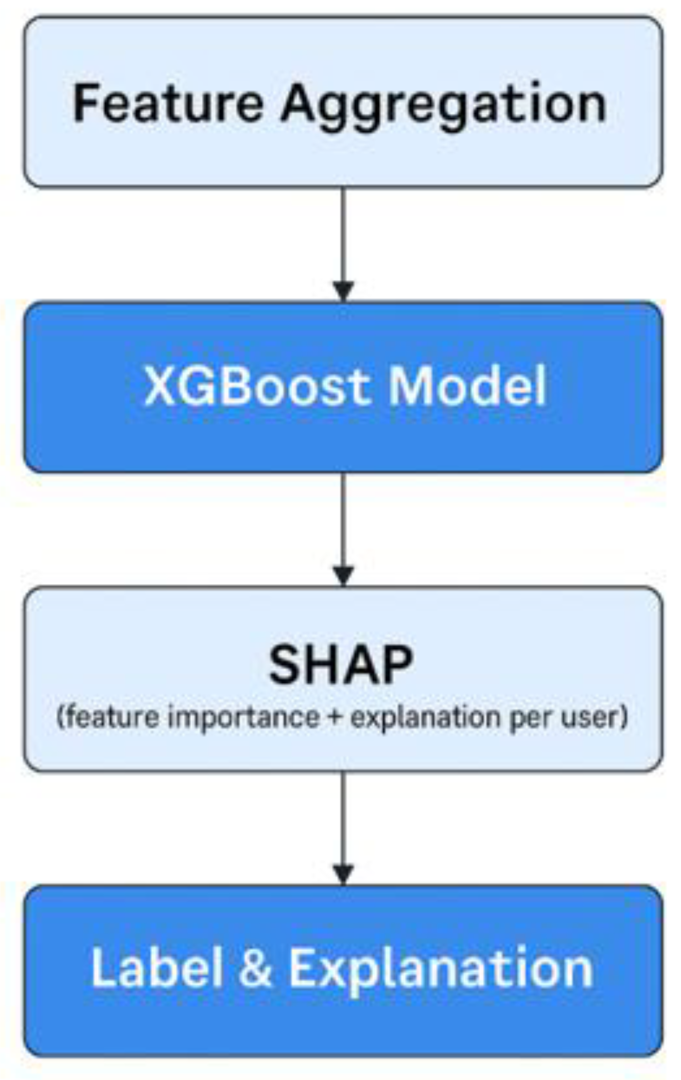
Figure 3.
Flowchart of RAG model which inherits SHAP features to generate human-language outputs.
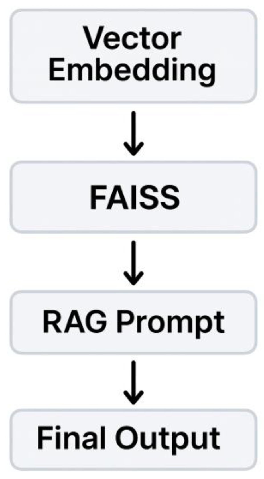
Figure 4.
Summary plot showing top features based on SHAP importance. Note. The feature ‘engage_tourn_WinningsT_mean’ was ranked as the third-most important feature but choosing ‘engage_cash_Windows_count’ as the third feature for addiction labeling allows for more variation in terms of types of behavioral interaction with gambling.
Figure 4.
Summary plot showing top features based on SHAP importance. Note. The feature ‘engage_tourn_WinningsT_mean’ was ranked as the third-most important feature but choosing ‘engage_cash_Windows_count’ as the third feature for addiction labeling allows for more variation in terms of types of behavioral interaction with gambling.
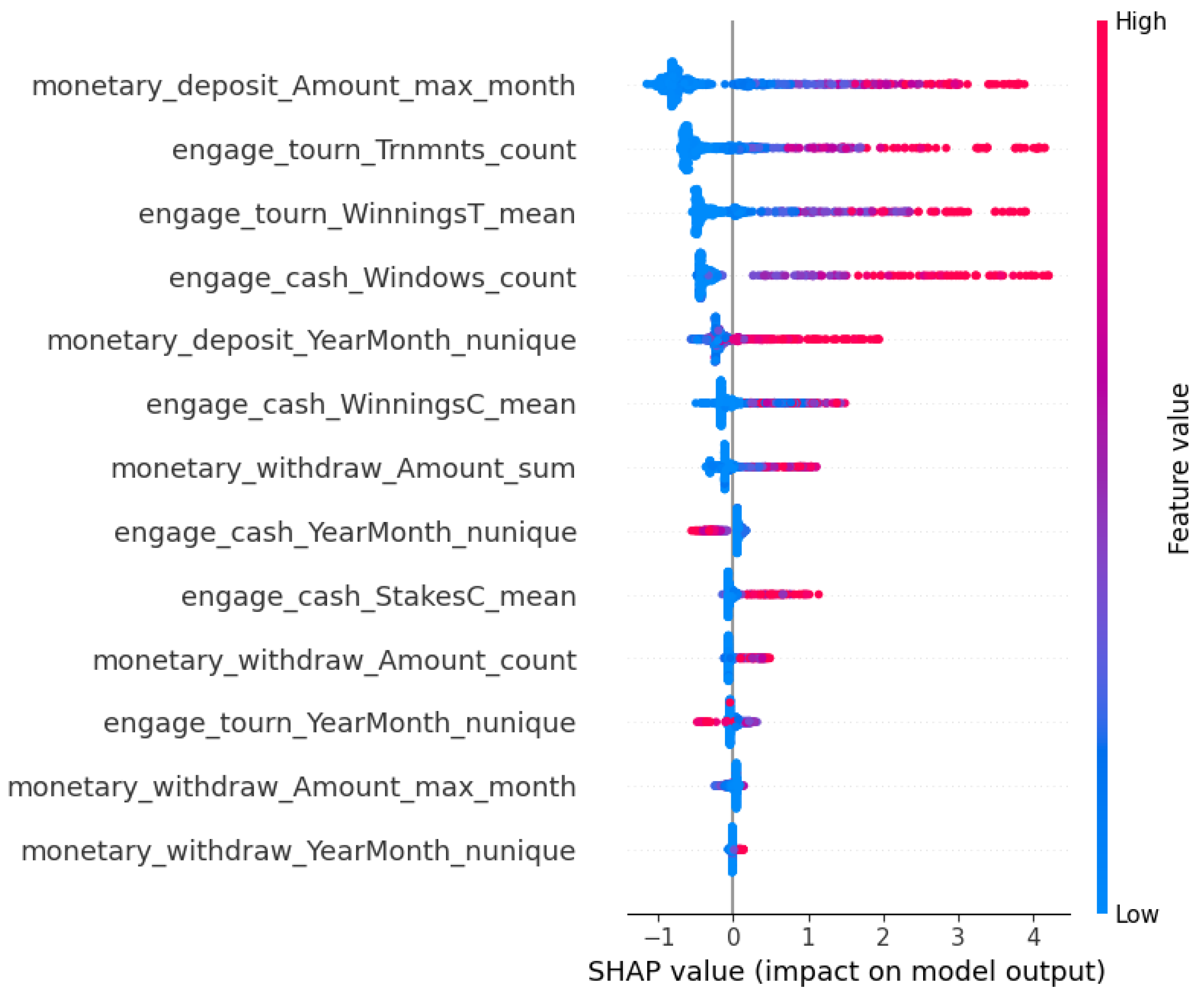
Figure 5.
Gambling addiction labeling logic.
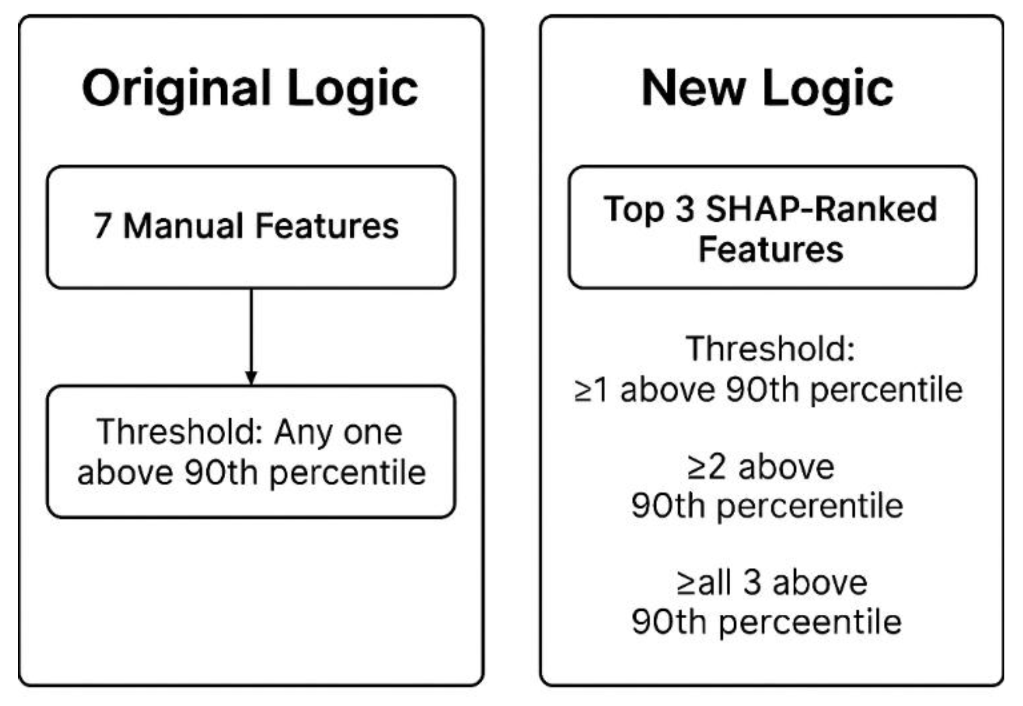
Figure 6.
Performance metrics of XGBoost model across 10 random seeds after tuning and modifications.
Figure 6.
Performance metrics of XGBoost model across 10 random seeds after tuning and modifications.
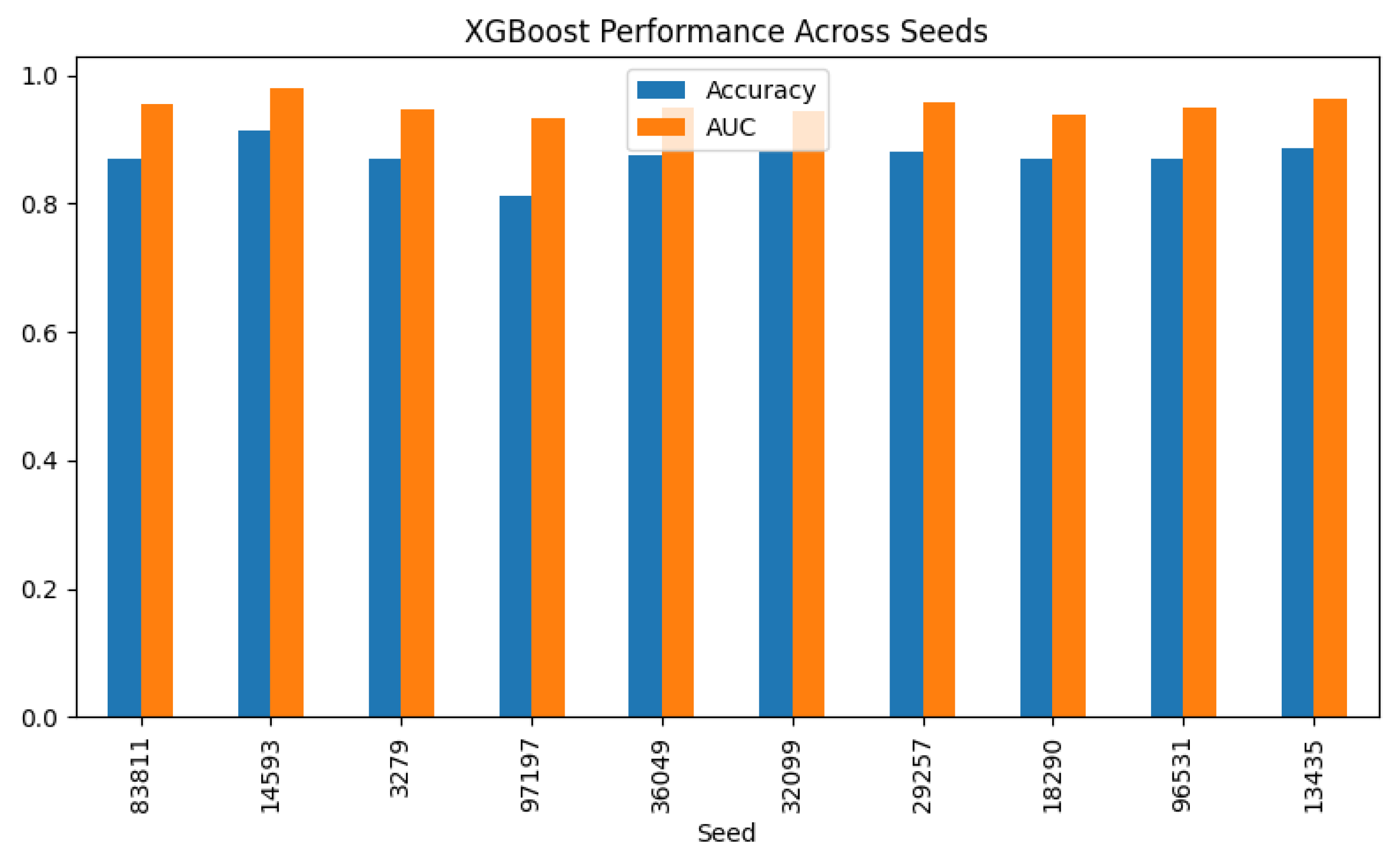
Figure 7.
Prevalence of addiction under manually selected features vs. SHAP-informed features.
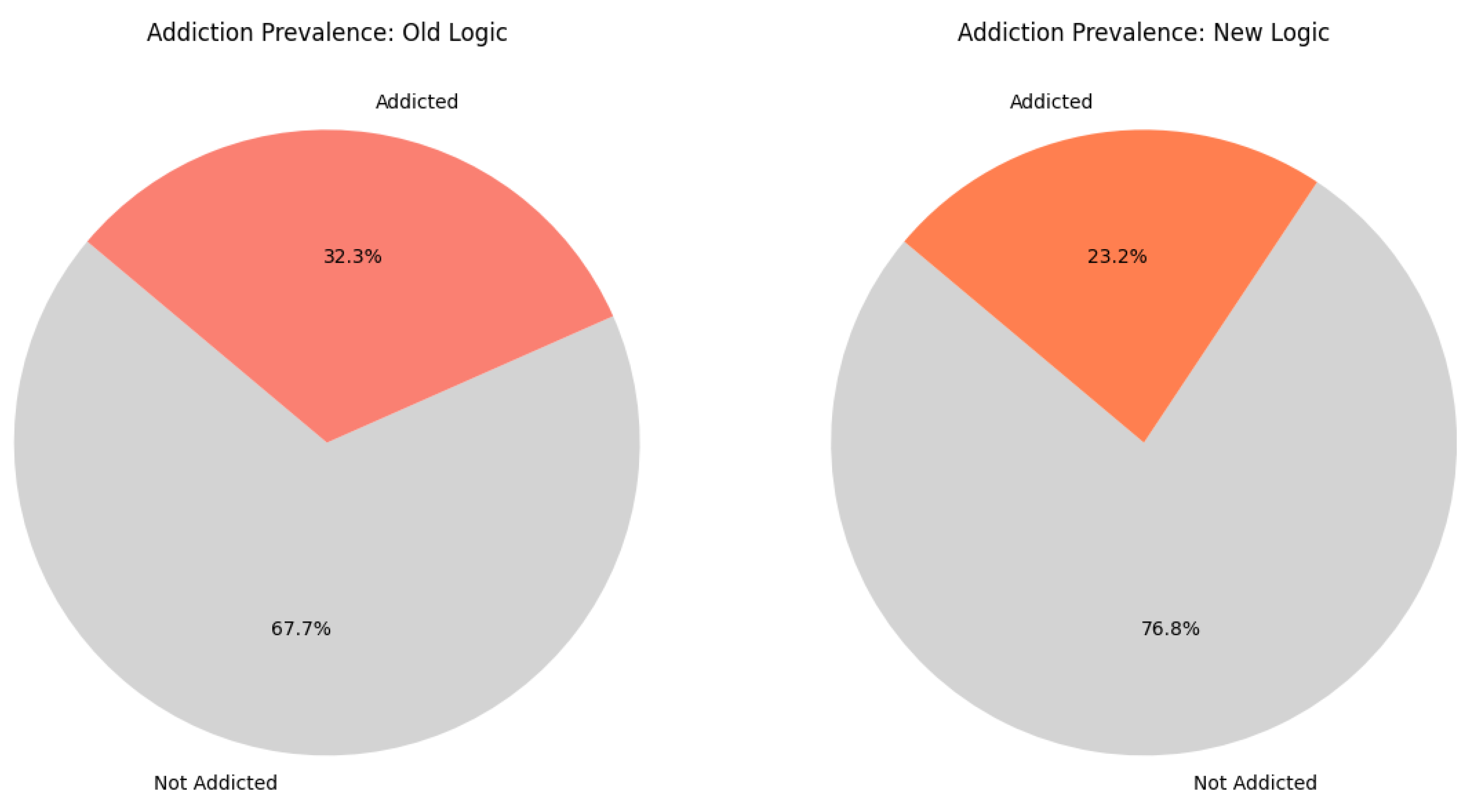
Figure 8.
Addiction labeling showing the total users and their categorizations. Note. The bar chart shows a total of 874 measured users in the study, where 282 users were labeled as addicted and 592 not addicted under the old logic. Switching to the new logic, 203 users were labeled as addicted and 671 not addicted. A total of 79 users were reclassified to not addicted. No new users were labeled as addicted under the SHAP logic.
Figure 8.
Addiction labeling showing the total users and their categorizations. Note. The bar chart shows a total of 874 measured users in the study, where 282 users were labeled as addicted and 592 not addicted under the old logic. Switching to the new logic, 203 users were labeled as addicted and 671 not addicted. A total of 79 users were reclassified to not addicted. No new users were labeled as addicted under the SHAP logic.
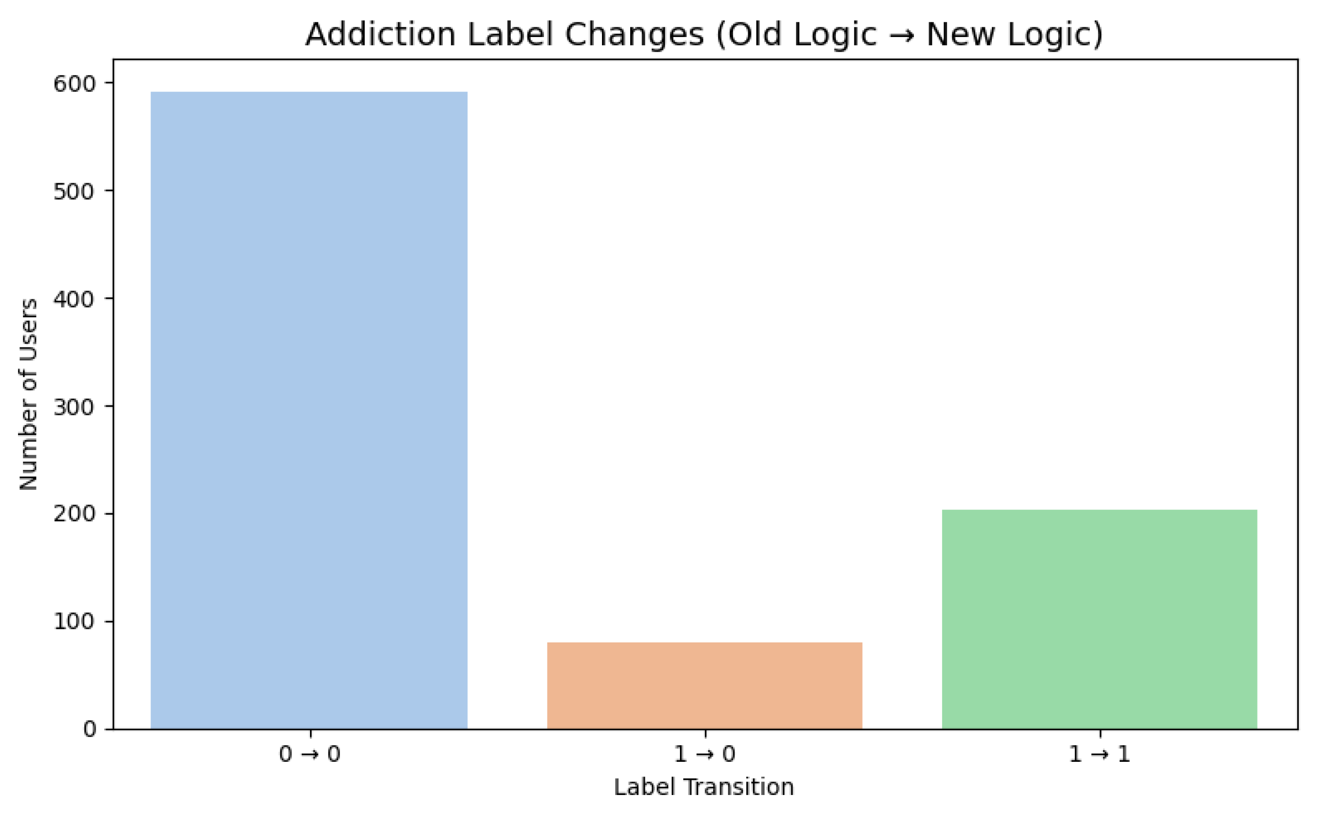
Figure 9.
Users categorized as addicted with a minimum of one, two, or all three features.
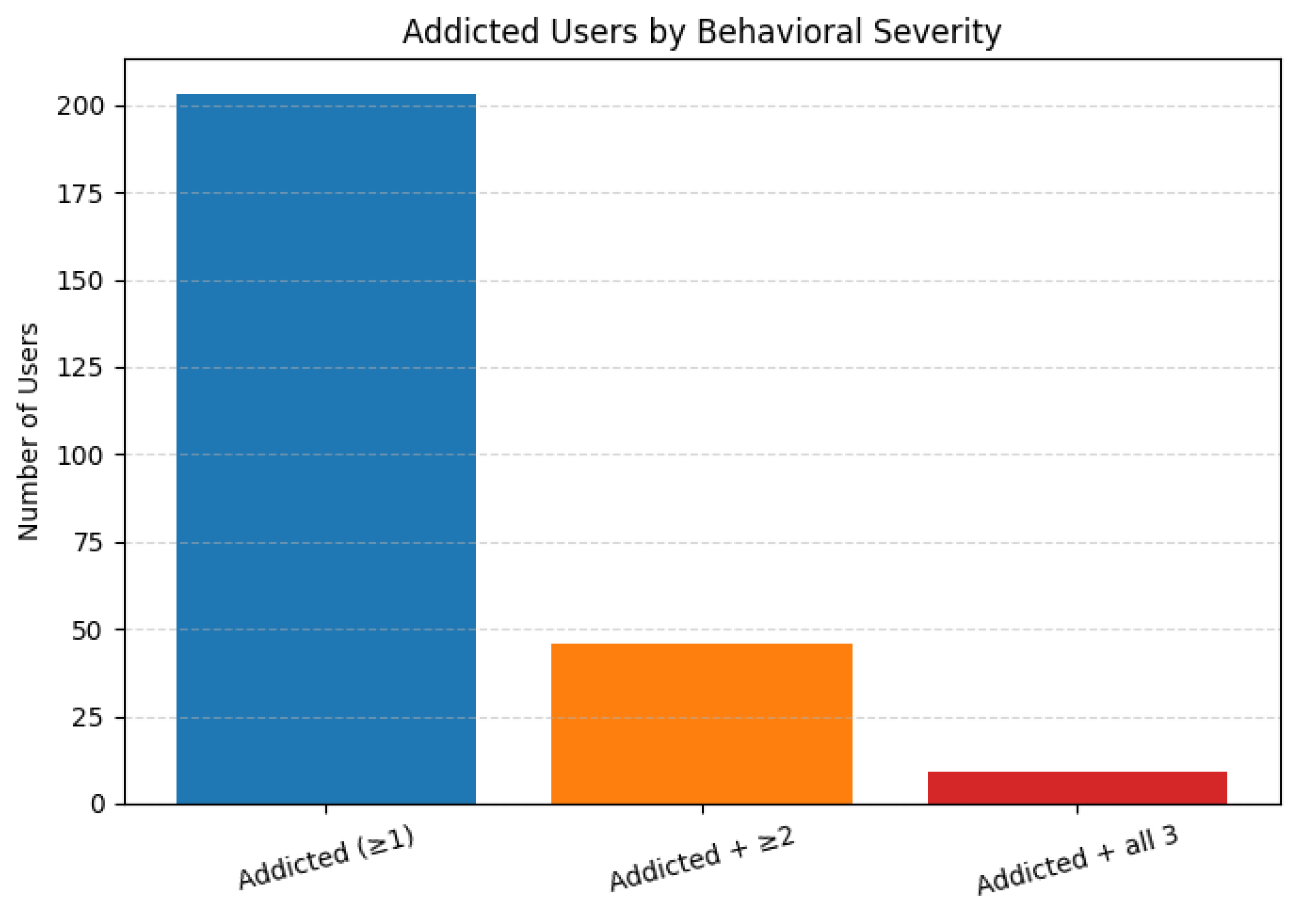
Figure 10.
Diagram of overlap between all addicted users and their specific addiction features. Note. Cash-only addicted users were 45. Tournament-only addicted users were 47. Deposit-only addicted users were 65. Cash & tournament addicted users were 23. Cash & deposit addicted users were 5. Tournament & Deposit addicted users were 9. Addicted to all three features were 9.
Figure 10.
Diagram of overlap between all addicted users and their specific addiction features. Note. Cash-only addicted users were 45. Tournament-only addicted users were 47. Deposit-only addicted users were 65. Cash & tournament addicted users were 23. Cash & deposit addicted users were 5. Tournament & Deposit addicted users were 9. Addicted to all three features were 9.
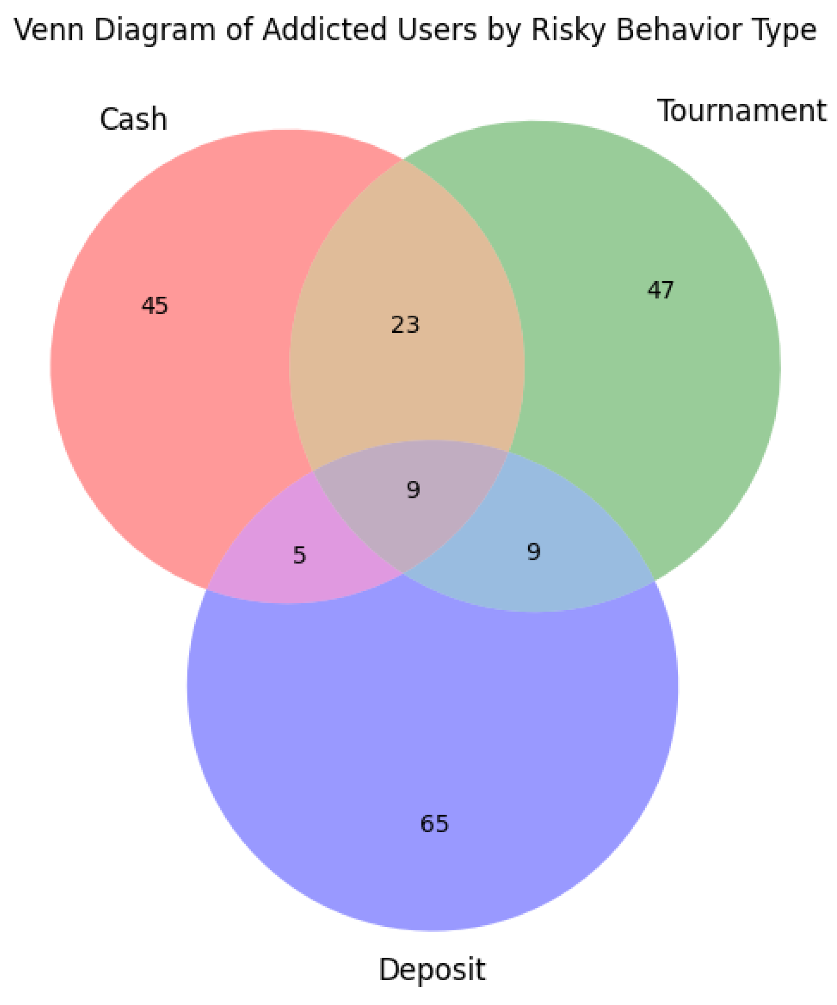
Figure 11.
Top-ranked stable SHAP features by median.
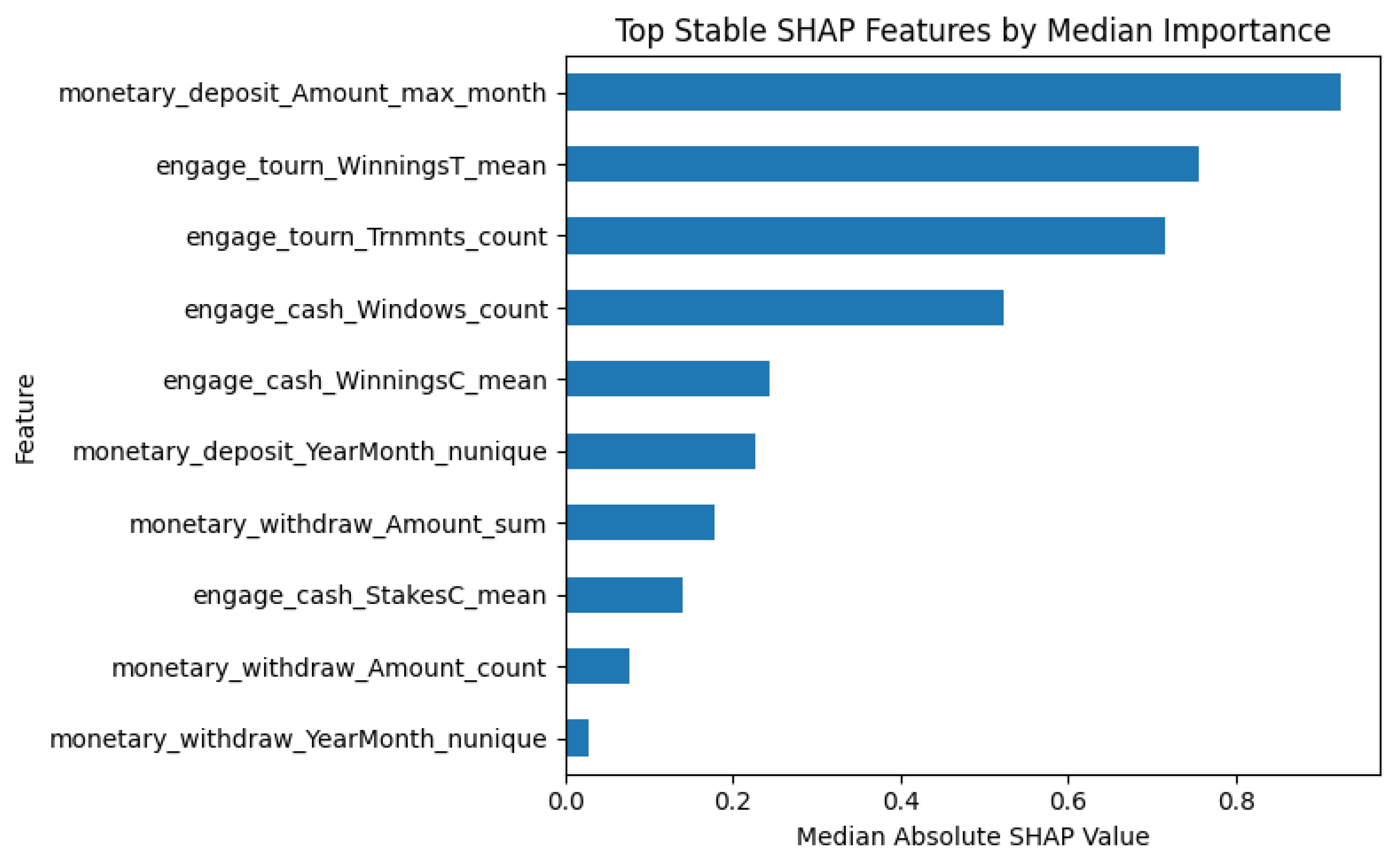
Figure 12.
Top-ranked stable features of XGBoost and SHAP, showing standard deviation and variance.
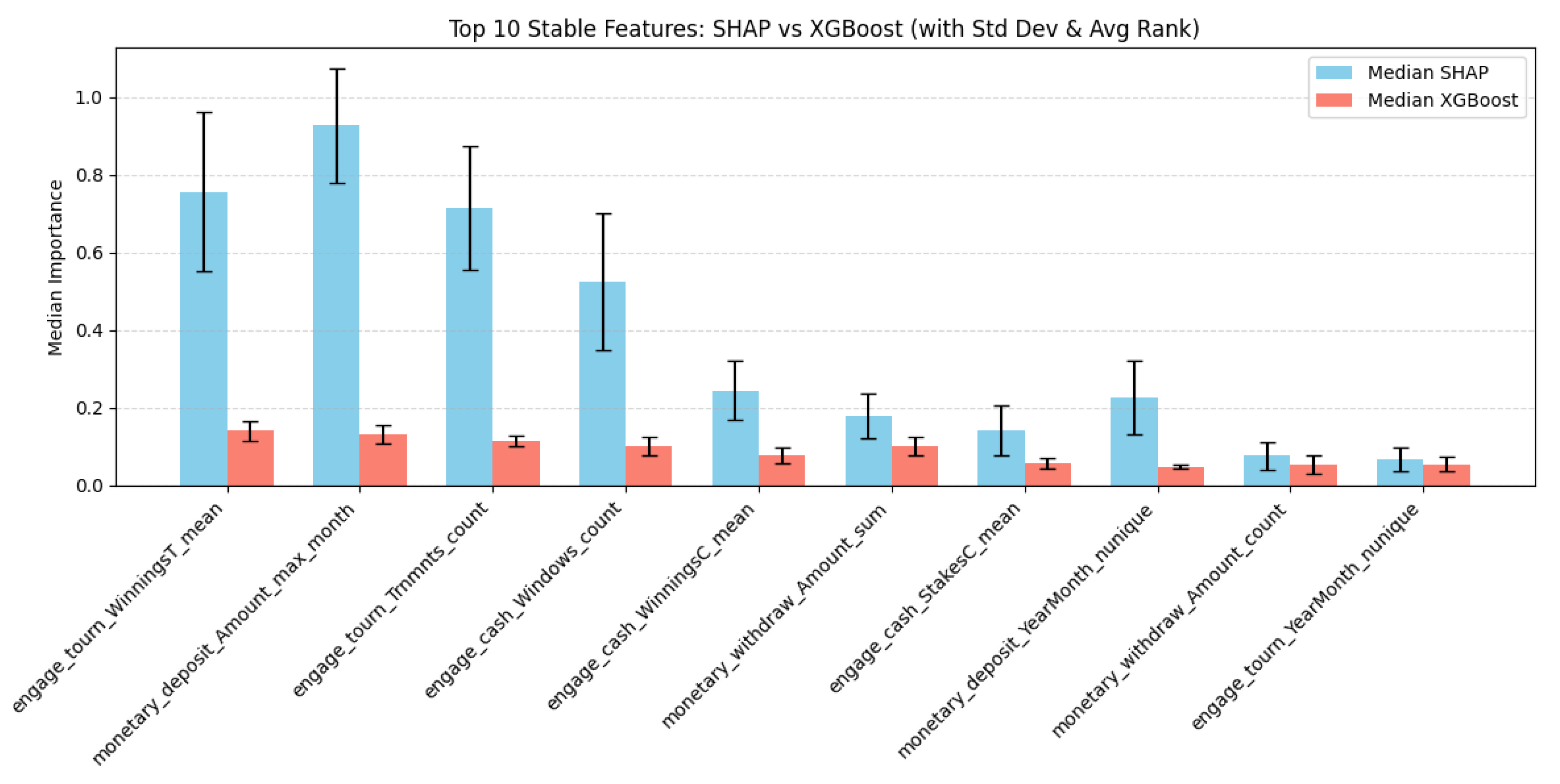
Figure 13.
Heatmap of addiction types by demographics (gender and age group). Note. This analysis accounts for all 874 users being measured in the study.
Figure 13.
Heatmap of addiction types by demographics (gender and age group). Note. This analysis accounts for all 874 users being measured in the study.
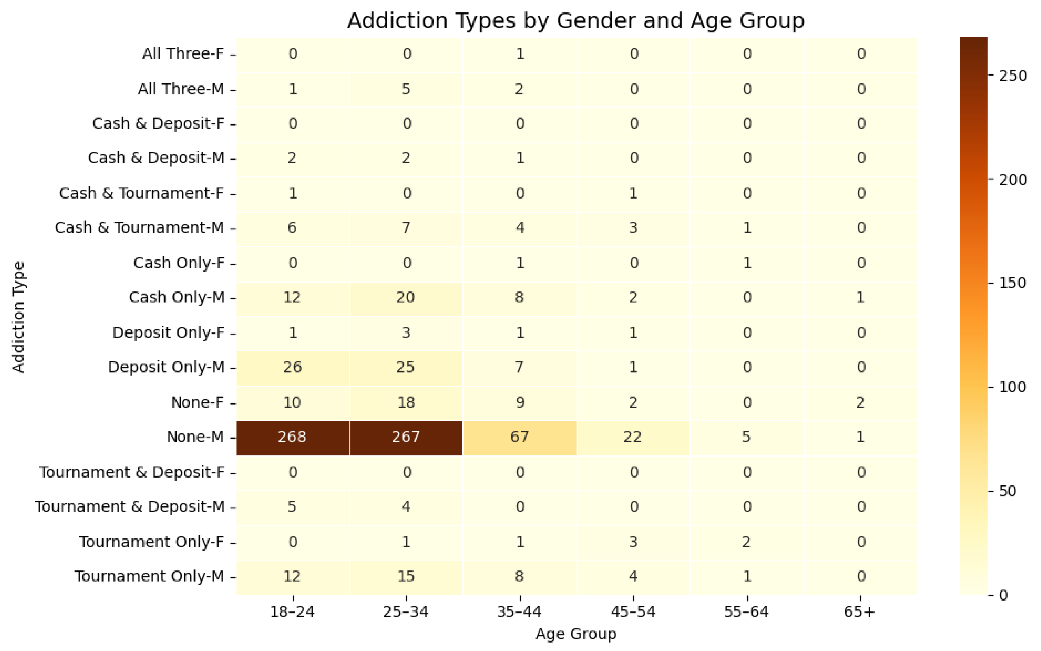

Table 1.
Mean behavioral feature values for users labeled as addicted and not addicted.
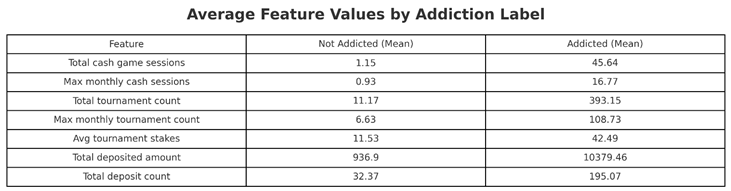 |
Note. Addicted users show significantly higher engagement across all measured dimensions—game volume, session bursts, deposit amounts, and tournament intensity—highlighting the behavioral thresholds used in the original (manual) labeling logic.
Table 2.
Evaluation of XGBoost – Performance-based Metrics by Seed.
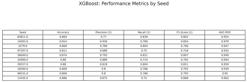 |
Table 3.
Evaluation of XGBoost – Mean and Variance of Metrics Across 10 seeds.
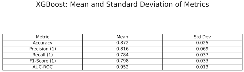 |
Table 4.
Highest-ranked SHAP features based on user-level individual engagement across 10 seeds.
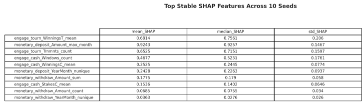 |
Table 5.
Classification report of SHAP-influenced language-based RAG system.
 |
Disclaimer/Publisher’s Note: The statements, opinions and data contained in all publications are solely those of the individual author(s) and contributor(s) and not of MDPI and/or the editor(s). MDPI and/or the editor(s) disclaim responsibility for any injury to people or property resulting from any ideas, methods, instructions or products referred to in the content. |
© 2025 by the authors. Licensee MDPI, Basel, Switzerland. This article is an open access article distributed under the terms and conditions of the Creative Commons Attribution (CC BY) license (http://creativecommons.org/licenses/by/4.0/).
Copyright: This open access article is published under a Creative Commons CC BY 4.0 license, which permit the free download, distribution, and reuse, provided that the author and preprint are cited in any reuse.


