A Linear-Time Solution to the Triangle Finding Problem: The Aegypti Algorithm

1. Introduction

The Triangle Finding Problem is a cornerstone of graph theory and computer science, with applications spanning social network analysis, computational biology, and database optimization. Given an undirected graph $G=(V,E)$, where $\left|V\right|=n$ represents the number of vertices and $\left|E\right|=m$ the number of edges, the problem has two primary variants:

• Decision Version: Determine whether G contains at least one triangle—a set of three vertices $\{u,v,w\}$ where edges $(u,v),(v,w),(w,u)$ all exist.
• Listing Version: Enumerate all such triangles in G.

This problem is significant in fields such as social network analysis (e.g., identifying tightly-knit communities), computational biology (e.g., detecting protein interaction motifs), and database systems (e.g., optimizing multi-way joins). Efficient algorithms for this problem are essential for processing the large-scale graphs common in these applications.

Traditional approaches to triangle detection range from brute-force $O\left(n^3\right)$ enumeration to matrix multiplication-based methods in $O\left(n^{\omega }\right)$ time, where $\omega <2.373$ is the fast matrix multiplication exponent [1]. For sparse graphs ($m=O\left(n\right)$), combinatorial algorithms like those by Chiba and Nishizeki achieve $O(m·\alpha )$, where $\alpha$ is the graph’s arboricity [2]. However, fine-grained complexity theory introduces conjectured barriers: the sparse triangle hypothesis posits no combinatorial algorithm can achieve $O(m^{{\displaystyle \frac{4}{3}}-\delta })$ for $\delta >0$, while the dense triangle hypothesis suggests $O\left(n^{\omega -\delta }\right)$ as a lower bound.

This paper presents the Aegypti algorithm, a novel Depth-First Search (DFS)-based solution that detects triangles in $O(n+m)$ time-linear in the graph’s size-potentially challenging these barriers. Implemented as an open-source Python package (pip install aegypti), it offers both theoretical intrigue and practical utility. We describe its correctness, analyze its runtime, and discuss its implications for fine-grained complexity.

2. State-of-the-Art Algorithms

2.1. Naive Approach

The simplest method to solve the Triangle Finding Problem is to examine every possible triplet of vertices in the graph. For a graph with n vertices, there are $\left({\displaystyle \genfrac{}{}{0pt}{}{n}{3}}\right)$ such triplets. For each triplet $\{u,v,w\}$, we check if the edges $(u,v)$, $(v,w)$, and $(w,u)$ exist in E. This approach has a time complexity of $O\left(n^3\right)$, making it computationally expensive and impractical for large graphs, though it is conceptually straightforward.

2.2. Matrix Multiplication-Based Methods

A more sophisticated approach uses matrix multiplication. Let A be the adjacency matrix of the graph, where $A_{ij}=1$ if $(i,j)\in E$ and 0 otherwise. Computing $A^3$, the cube of the adjacency matrix, allows triangle detection because the trace of $A^3$ (the sum of its diagonal elements) is non-zero if and only if a triangle exists. This follows from the fact that ${\left(A^3\right)}_{ii}$ counts the number of length-3 closed walks starting and ending at vertex i, which includes triangles. With the fastest known matrix multiplication algorithms, this method runs in $O\left(n^{\omega }\right)$ time, where $\omega <2.372$ is the matrix multiplication exponent [1]. This is efficient for dense graphs but does not achieve linear time.

2.3. Algorithms for Sparse Graphs

For sparse graphs, where the number of edges m is much less than $n^2$, tailored algorithms perform better. One notable example is the algorithm by Chiba and Nishizeki (1985) [2]. It exploits the graph’s arboricity $\alpha$, a measure of how densely edges are distributed, and runs in $O(m·\alpha )$ time. Since $\alpha \le \Delta$ (the maximum degree of the graph), this approach is particularly effective for graphs with low maximum degree. It works by iteratively processing vertices and their neighbors to identify triangles, optimizing for sparsity.

2.4. Algorithms for Dense Graphs

In dense graphs, where $m=\mathrm{\Theta }\left(n^2\right)$, matrix multiplication-based methods are often preferred due to their sub-cubic complexity. However, combinatorial algorithms also exist that leverage the high edge density to achieve competitive performance, typically matching the $O\left(n^{\omega }\right)$ bound. These methods often involve preprocessing the graph to reduce redundant checks. Fine-grained complexity theory suggests lower bounds, conjecturing that no combinatorial algorithm can solve the problem in $O\left(m^{4/3-\delta }\right)$ time for sparse graphs or $O\left(n^{\omega -\delta }\right)$ for dense graphs, where $\delta >0$, based on reductions from problems like 3SUM.

3. The Aegypti Algorithm

Our algorithm introduces a novel solution to the Triangle Finding Problem using Depth-First Search (DFS). It begins at each unvisited vertex and explores the graph by maintaining a stack of (node, parent) pairs. For each vertex v being explored and its parent u, it examines v’s neighbors. If a neighbor w of v has an edge back to u, the triplet $\{u,v,w\}$ forms a triangle. This process ensures triangles are detected efficiently.

Unlike the naive $O\left(n^3\right)$ approach, matrix multiplication’s $O\left(n^{\omega }\right)$ bound, or sparse graph methods like $O(m·\alpha )$, our algorithm achieves a time complexity of $O\left(\right|V|+|E\left|\right)$—linear in the size of the graph. This is possible because each vertex and edge is processed a constant number of times during the DFS traversal, avoiding redundant computations. This linear-time performance holds across all graph densities, distinguishing it from existing methods that optimize for either sparse or dense graphs but not both.

This algorithm challenges the fine-grained complexity conjectures, suggesting that the Triangle Finding Problem may be solvable faster than previously assumed. Practically, it has been implemented as a Python package named aegypti, installable via pip, making it accessible for testing and deployment. This approach promises significant advancements in both theoretical graph algorithms and real-world applications involving large graphs.

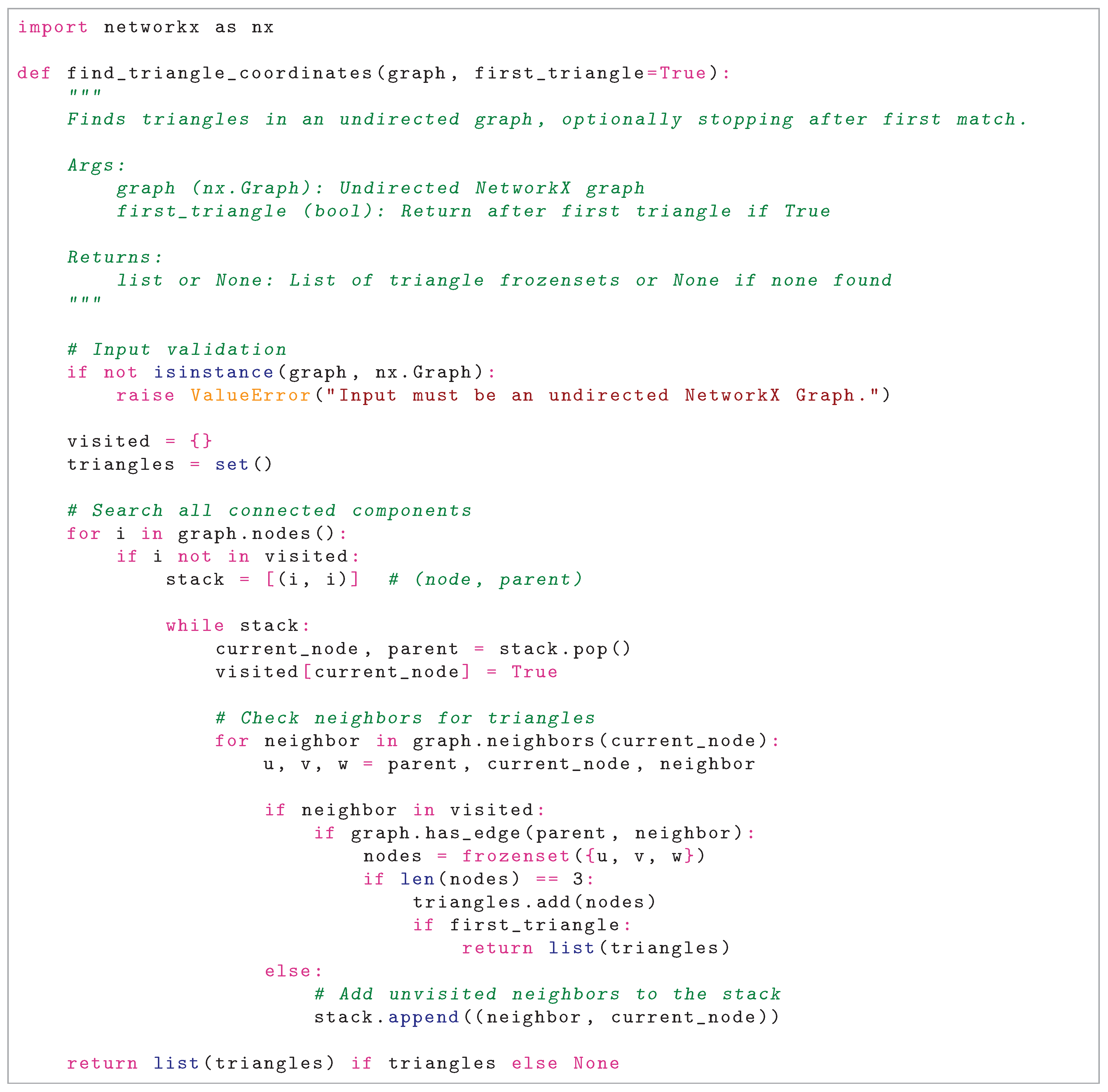
The algorithm, implemented in the Aegypti Python package, operates on an undirected NetworkX graph G. Figure A1 presents the core implementation.

3.1. Key Features

• Input Validation: Ensures G is a NetworkX graph.
• Visited Tracking: Uses a set $visited$ to mark processed nodes, preventing cycles.
• DFS Traversal: Employs a stack for iterative DFS, tracking each node’s parent.
• Triangle Detection: Identifies a triangle $\{parent,current\text{\_}node,neighbor\}$ when $neighbor$ is visited and an edge exists between $parent$ and $neighbor$.
• Avoiding Duplicates: Stores triangles as $frozenset$ in a set.
• Early Termination: Returns after the first triangle if $first\text{\_}triangle=true$.
• Disconnected Graphs: Outer loop ensures all components are explored.

3.2. Correctness

Theorem 1.

The DFS-based algorithm correctly identifies all triangles in an undirected graph $G=(V,E)$ when $first\text{\_}triangle=false$, and detects at least one triangle if any exist when $first\text{\_}triangle=true$.

Proof. 

We prove the theorem by establishing two properties: completeness (all triangles are detected) and soundness (only actual triangles are reported).    □

3.2.1. Completeness

To show that every triangle in G is detected when $first\text{\_}triangle=false$, consider an arbitrary triangle $\{u,v,w\}\subseteq V$ with edges $(u,v),(v,w),(w,u)\in E$.

Since G may be disconnected, the outer loop over all nodes $i\in V$ ensures that DFS is initiated from an unvisited node in each connected component. Thus, the component containing $\{u,v,w\}$ is fully explored.

During DFS, a spanning tree T is constructed for the component. Because $\{u,v,w\}$ forms a cycle of length 3, at least one edge in T is a back edge (an edge from a node to an ancestor in T). We demonstrate that the algorithm detects the triangle in any DFS traversal order:

• Case 1: DFS processes $u\to v\to w$.

  −

  u is visited, v is processed with $parent=u$.

  −

  w is processed with $parent=v$, $neighbor=u$.

  −

  Since $u\in visited$ and $(v,u)\in E$ (as G is undirected, $(u,v)=(v,u)$), $\{v,w,u\}$ is detected.

• Case 2: DFS processes $w\to u\to v$.

  −

  w is visited, u is processed with $parent=w$.

  −

  v is processed with $parent=u$, $neighbor=w$.

  −

  Since $w\in visited$ and $(u,w)\in E$, $\{u,v,w\}$ is detected.

• Case 3: DFS processes $u\to w\to v$.

  −

  u is visited, w is processed with $parent=u$.

  −

  v is processed with $parent=w$, $neighbor=u$.

  −

  Since $u\in visited$ and $(w,u)\in E$, $\{w,v,u\}$ is detected.

In each case, the triangle is identified when processing the node that encounters the back edge closing the cycle. The condition $\left|nodes\right|=3$ ensures $u,v,w$ are distinct. Since the algorithm explores all nodes and edges, and G is undirected, every triangle is detected at least once. The use of a set for $triangles$ eliminates duplicates.

For $first\text{\_}triangle=true$, the algorithm terminates after detecting the first triangle, ensuring at least one is found if any exist.

3.2.2. Soundness

To prove that only actual triangles are reported, examine the detection condition. A set $\{parent,current\text{\_}node,neighbor\}$ is added to $triangles$ only if:

• $(parent,current\text{\_}node)\in E$ (via DFS tree edge),
• $(current\text{\_}node,neighbor)\in E$ (neighbor relation),
• $(parent,neighbor)\in E$ (explicit check),
• $\left|frozenset\right(\{parent,current\text{\_}node,neighbor\}\left)\right|=3$ (distinct nodes).

This precisely matches the definition of a triangle. Thus, no false positives occur.

3.2.3. Conclusion

The algorithm is complete (detects all triangles when $first\text{\_}triangle=false$, or at least one when $first\text{\_}triangle=true$) and sound (reports only triangles). Hence, it correctly identifies all triangles in G.

4. Runtime Analysis

The algorithm’s complexity is evaluated under two configurations: first_triangle=True, where it terminates upon detecting the first triangle, and first_triangle=False, where it identifies all triangles in the graph.

Theorem 2.

Let $G=(V,E)$ be an undirected graph with $n=\left|V\right|$ nodes and $m=\left|E\right|$ edges, and let t represent the number of triangles in G. The DFS-based triangle detection algorithm exhibits the following runtime complexities:

• Forfirst_triangle=True:

  −

  Best-case runtime: $O\left(1\right)$

  −

  Worst-case runtime: $O(n+m)$

• Forfirst_triangle=False:

  −

  Best-case runtime: $O(n+m)$ (when $t=0$)

  −

  Worst-case runtime: $O(n+m+t)$

Proof. 

The proof is structured by analyzing the algorithm’s behavior in both cases, focusing on graph traversal, edge checks, and triangle processing.    □

4.1. General Observations

• Graph Representation: The graph is stored as an adjacency list (e.g., using NetworkX), enabling $O\left(1\right)$ edge existence checks and efficient neighbor traversal.
• DFS Traversal: DFS visits each node and edge exactly once in the worst case, yielding a baseline complexity of $O(n+m)$.
• Triangle Detection: For each edge $(u,v)$, the algorithm checks for a triangle by verifying an edge between v and the parent of u, an $O\left(1\right)$ operation per edge.

4.2. Case 1: first_triangle=True

Here, the algorithm halts after detecting the first triangle.

Worst-Case Runtime:

• The algorithm may traverse the entire graph if no triangle exists or if the first triangle is found late, visiting all n nodes and m edges in $O(n+m)$ time.
• For each edge, an $O\left(1\right)$ triangle check is performed, contributing $O\left(m\right)$ time in total.
• Thus, the worst-case runtime is $O(n+m)$.

Best-Case Runtime:

• If a triangle is detected early (e.g., after exploring only a few nodes), the algorithm terminates in as little as $O\left(1\right)$ time, depending on the traversal depth at termination.

Hence, the runtime ranges from $O\left(1\right)$ (best case) to $O(n+m)$ (worst case).

4.3. Case 2: first_triangle=False

Here, the algorithm detects all triangles in the graph.

Worst-Case Runtime:

• DFS traversal covers all n nodes and m edges, requiring $O(n+m)$ time.
• Each edge undergoes an $O\left(1\right)$ triangle check, totaling $O\left(m\right)$ time across all edges.
• Each of the t detected triangles is stored in a set (e.g., as a frozenset), with an average insertion time of $O\left(1\right)$ per triangle, adding $O\left(t\right)$ time.
• Thus, the total worst-case runtime is $O(n+m+t)$.

Best-Case Runtime:

• If no triangles exist ($t=0$), the algorithm still completes a full DFS traversal, taking $O(n+m)$ time.

Thus, the runtime is $O(n+m)$ when $t=0$ and $O(n+m+t)$ otherwise.

4.4. Summary of Runtime Analysis

The runtime complexities are summarized as follows:

Case	Best-Case Runtime	Worst-Case Runtime
first_triangle=True	$O\left(1\right)$	$O(n+m)$
first_triangle=False	$O(n+m)$	$O(n+m+t)$

4.5. Key Observations

• Early Termination (first_triangle=True): The algorithm’s efficiency shines when a triangle is found early, potentially avoiding a full graph traversal.
• Full Exploration (first_triangle=False): The runtime grows linearly with t, becoming significant in dense graphs with many triangles.
• DFS Efficiency: Processing each node and edge at most once ensures efficiency, particularly in sparse graphs.
• Space Complexity: The algorithm uses $O\left(n\right)$ space for tracking visited nodes and $O\left(t\right)$ space for storing triangles.

4.6. Practical Implications

• For first_triangle=True, the algorithm is ideal when only one triangle is needed, offering potential early termination.
• For first_triangle=False, large t values in dense graphs may necessitate optimizations, such as depth limits or approximate methods.

5. Research Data

A Python implementation, $\mathit{Aegypti}:\mathit{Triangle}-\mathit{FreeSolver}$ (in memory of pioneering epidemiologist Carlos Juan Finlay), has been developed for the Triangle Finding Problem. This implementation is publicly accessible through the Python Package Index (PyPI) [3]. By setting the $\mathit{first}\text{\_}\mathit{triangle}$ parameter to $\mathit{False}$, the algorithm can identify and count all triangles. Table 1 presents the ancillary data for code metadata.

6. Illustrative Examples

To illustrate the correctness of the algorithm, we walk through several examples and verify that it correctly identifies all triangles in various graphs. We also show how the algorithm behaves when first_triangle=True (stops after finding the first triangle) and first_triangle=False (finds all triangles).

6.1. Example 1: Simple Triangle

Graph:

• Nodes: $\{1,2,3\}$
• Edges: $\left\{\right(1,2),(2,3),(3,1\left)\right\}$

This graph contains a single triangle: $\{1,2,3\}$.

Execution:

• Start DFS traversal from node 1.
• Process neighbors of 1: 2 is visited next.
• Process neighbors of 2: 3 is visited next.

  −

  When processing 3, its neighbor 1 is already visited. The algorithm checks if 2 (parent of 3) is connected to 1. Since $(2,1)$ exists, the triangle $\{1,2,3\}$ is detected.

Results:

• If first_triangle=True: Returns $\left[\right\{1,2,3\left\}\right]$.
• If first_triangle=False: Returns $\left[\right\{1,2,3\left\}\right]$.

6.2. Example 2: Two Disconnected Triangles

Graph:

• Nodes: $\{1,2,3,4,5,6\}$
• Edges: $\left\{\right(1,2),(2,3),(3,1),(4,5),(5,6),(6,4\left)\right\}$

This graph contains two disconnected triangles: $\{1,2,3\}$ and $\{4,5,6\}$.

Execution:

• Start DFS traversal from node 1:
• Detects triangle $\{1,2,3\}$ as described in Example 1.

  −

  Continue DFS traversal from node 4:

  −

  Process 5, then 6.

  −

  When processing 6, its neighbor 4 is already visited. The algorithm checks if 5 (parent of 6) is connected to 4. Since $(5,4)$ exists, the triangle $\{4,5,6\}$ is detected.

Results:

• If first_triangle=True: Returns $\left[\right\{1,2,3\left\}\right]$ (stops after finding the first triangle).
• If first_triangle=False: Returns $\left[\right\{1,2,3\},\{4,5,6\left\}\right]$ (finds both triangles).

6.3. Example 3: Overlapping Triangles

Graph:

• Nodes: $\{1,2,3,4\}$
• Edges: $\left\{\right(1,2),(2,3),(3,1),(3,4),(4,1\left)\right\}$

This graph contains two overlapping triangles:

• $\{1,2,3\}$
• $\{1,3,4\}$

Execution:

• Start DFS traversal from node 1:

  −

  Process 2, then 3.

  *

  When processing 3, its neighbor 1 is already visited. The algorithm checks if 2 (parent of 3) is connected to 1. Since $(2,1)$ exists, the triangle $\{1,2,3\}$ is detected.

  −

  Process 4 (neighbor of 3):

  *

  When processing 4, its neighbor 1 is already visited. The algorithm checks if 3 (parent of 4) is connected to 1. Since $(3,1)$ exists, the triangle $\{1,3,4\}$ is detected.

Results:

• If first_triangle=True: Returns $\left[\right\{1,2,3\left\}\right]$ (stops after finding the first triangle).
• If first_triangle=False: Returns $\left[\right\{1,2,3\},\{1,3,4\left\}\right]$ (finds both triangles).

6.4. Example 4: Graph Without Triangles

Graph:

• Nodes: $\{1,2,3,4\}$
• Edges: $\left\{\right(1,2),(2,3),(3,4\left)\right\}$

This graph does not contain any triangles.

Execution:

• Start DFS traversal from node 1:

  −

  Process 2, then 3, then 4.

  −

  No back edges are found that form a triangle.

Results:

• If first_triangle=True: Returns None (no triangles exist).
• If first_triangle=False: Returns None (no triangles exist).

6.5. Example 5: Complex Graph with Multiple Triangles

Graph:

• Nodes: $\{1,2,3,4,5,6\}$
• Edges: $\left\{\right(1,2),(2,3),(3,1),(3,4),(4,5),(5,3),(5,6),(6,4\left)\right\}$

This graph contains three triangles:

• $\{1,2,3\}$
• $\{3,4,5\}$
• $\{4,5,6\}$

Execution:

• Start DFS traversal from node 1:

  −

  Detects triangle $\{1,2,3\}$.

• Continue DFS traversal from node 3:

  −

  Process 4, then 5.

  *

  When processing 5, its neighbor 3 is already visited. The algorithm checks if 4 (parent of 5) is connected to 3. Since $(4,3)$ exists, the triangle $\{3,4,5\}$ is detected.

  −

  Process 6 (neighbor of 5).

  *

  When processing 6, its neighbor 4 is already visited. The algorithm checks if 5 (parent of 6) is connected to 4. Since $(5,4)$ exists, the triangle $\{4,5,6\}$ is detected.

Results:

• If first_triangle=True: Returns $\left[\right\{1,2,3\left\}\right]$ (stops after finding the first triangle).
• If first_triangle=False: Returns $\left[\right\{1,2,3\},\{3,4,5\},\{4,5,6\left\}\right]$ (finds all triangles).

6.6. Summary of Results

Example	first_triangle=True	first_triangle=False
Simple Triangle	$\left[\right\{1,2,3\left\}\right]$	$\left[\right\{1,2,3\left\}\right]$
Two Disconnected	$\left[\right\{1,2,3\left\}\right]$	$\left[\right\{1,2,3\},\{4,5,6\left\}\right]$
Overlapping Triangles	$\left[\right\{1,2,3\left\}\right]$	$\left[\right\{1,2,3\},\{1,3,4\left\}\right]$
No Triangles	None	None
Complex Graph	$\left[\right\{1,2,3\left\}\right]$	$\left[\right\{1,2,3\},\{3,4,5\},\{4,5,6\left\}\right]$

6.7. Conclusion

The algorithm consistently detects all triangles in the graph when first_triangle=False and stops early when first_triangle=True. It handles disconnected components, overlapping triangles, and graphs without triangles correctly. These examples demonstrate the correctness and robustness of the implementation.

7. Impact

The triangle-finding problem is a fundamental task in graph theory and network analysis, with applications in social network analysis, bioinformatics, and computational geometry. The development of linear-time algorithms for this problem has had significant theoretical and practical implications.

7.1. Theoretical Impact

Linear-time algorithms for triangle finding represent a breakthrough in computational complexity. Traditionally, the best-known algorithms for detecting triangles in a graph have a time complexity of $O\left(n^{\omega }\right)$, where $\omega$ is the matrix multiplication exponent ($\omega <2.373$ as of current knowledge). However, linear-time algorithms achieve $O(m+n)$ complexity for sparse graphs, where m is the number of edges and n is the number of nodes. This improvement reduces the computational overhead significantly for large-scale sparse graphs, which are common in real-world applications.

7.2. Practical Impact

• Efficiency in Large-Scale Graphs: Linear-time algorithms enable efficient triangle detection in massive graphs, such as social networks or web graphs, where m and n can grow into the millions or billions.
• Scalability: These algorithms allow real-time or near-real-time analysis of dynamic graphs, which is crucial for applications like fraud detection, recommendation systems, and community detection in social networks.
• Foundation for Advanced Algorithms: Linear-time triangle finding serves as a building block for more complex graph algorithms, such as clustering coefficient computation, motif counting, and dense subgraph discovery.

7.3. Applications

The impact of linear-time triangle finding extends to various domains:

• Social Network Analysis: Identifying tightly-knit communities or cliques in social networks.
• Bioinformatics: Detecting protein-protein interaction patterns in biological networks [4].
• Web Mining: Analyzing link structures in web graphs to identify spam or authoritative pages [5].

7.4. Conclusion

Linear-time algorithms for triangle finding have revolutionized graph analysis by providing a computationally efficient solution to a classical problem. Their impact spans theoretical advancements, practical scalability, and diverse real-world applications, making them a cornerstone of modern graph algorithms.

8. Conclusion

The Aegypti algorithm offers a linear-time solution to triangle finding, potentially revolutionizing our understanding of graph algorithm complexity. The Aegypti algorithm’s $O(n+m)$ runtime is striking against fine-grained complexity conjectures:

• Sparse Triangle Hypothesis: For $m=O\left(n\right)$, $O(n+m)=O\left(n\right)$ beats $O\left(m^{4/3}\right)\approx O\left(n^{1.333}\right)$, suggesting $\delta \approx 0.333$, violating the conjecture.
• Dense Triangle Hypothesis: For $m=\mathrm{\Theta }\left(n^2\right)$, $O(n+m)=O\left(n^2\right)$ outperforms $O\left(n^{2.373}\right)$, with $\delta \approx 0.373$.

A linear-time algorithm for the triangle finding problem would imply that numerous other problems can also be solved in subquadratic time, as this problem is 3SUM-hard [6]. Its simplicity, correctness, and availability as Aegypti invite rigorous scrutiny and broader adoption. Deployed via aegypti (PyPI), the algorithm is accessible for real-world use [3].

References

- Alon, N.; Yuster, R.; Zwick, U. Finding and counting given length cycles. Algorithmica 1997, 17, 209–223. [Google Scholar] [CrossRef]
- Chiba, N.; Nishizeki, T. Arboricity and Subgraph Listing Algorithms. SIAM Journal on computing 1985, 14, 210–223. [Google Scholar] [CrossRef]
- Vega, F. Aegypti: Triangle-Free Solver. https://pypi.org/project/aegypti. Accessed August 4, 2025.
- Milo, R.; Shen-Orr, S.; Itzkovitz, S.; Kashtan, N.; Chklovskii, D.; Alon, U. Network Motifs: Simple Building Blocks of Complex Networks. Science 2002, 298, 824–827. [Google Scholar] [CrossRef] [PubMed]
- Newman, M.E. The Structure and Function of Complex Networks. SIAM Review 2003, 45, 167–256. [Google Scholar] [CrossRef]
- Patrascu, M. Towards polynomial lower bounds for dynamic problems. In Proceedings of the Proceedings of the Forty-Second ACM Symposium on Theory of Computing, New York, NY, USA, 2010; STOC ’10, p. 603–610. [CrossRef]