Three-Dimensional Architecture of Foreland Basins from Seismic Noise Recording: Tectonic Implications for the Western End of the Guadalquivir Basin

David Amador Luna; Albert Macau; Carlos Fernández; Francisco M. Alonso-Chaves

doi:10.20944/preprints202506.0810.v1

Submitted:

09 June 2025

Posted:

10 June 2025

You are already at the latest version

Abstract

The Variscan and Mesozoic basement are covered by Neogene and Quaternary sediments belonging to the Guadalquivir foreland Basin (southern Spain). This study explores the subsurface of its westernmost sector using the HVSR method, recording seismic noise at 334 stations between the mouths of the Guadiana and the Guadalquivir rivers, near Doñana National Park. Fundamental frequency and basement measurements enabled the estimation of an empirical formula for basement depth: h = 80.16·f0-1.48. Five distinct HVSR responses were obtained: (a) low-frequency peaks, indicating deep substratum; (b) high-frequency peaks, shallow bedrock; (c) broad peaks, potential critical zones (3D-2D effects); (d) double peaks (marshlands); and (e) no peaks, near-outcropping bedrock. The soil fundamental frequencies range from 0.23 to 18 Hz, with bedrock depth ranges from 1–5 meters in the northwest to over 600 meters in the southeast. Borehole data correlate strongly with HVSR-derived results, with typical discrepancies of only a few tens of meters, likely due to the presence of not-geological basement acting as a mechanical. Although the possibility of ancient fluvial terraces of the Guadalquivir River contributing to abrupt slope changes is considered, H/V spectra with broad peaks suggest tectonic origins. This study presents the first three-dimensional model of the basin basement over an area exceeding 2,300 km², revealing a horst-and-graben system formed by foreland deformation linked to the westward advance of the Rif-Betic orogenic front.

Keywords:

HVSR method

;

seismic noise

;

Guadalquivir Basin

;

fundamental frequency

;

3-D model

;

horst-graben system

Subject:

Environmental and Earth Sciences - Geophysics and Geology

1. Introduction

Passive seismic techniques based on the analysis and interpretation of seismic noise recorded by triaxial seismometers have proven to be valuable tools for studying the mechanical properties of soil. The Horizontal-to-Vertical Spectral Ratio (HVSR), also known as the H/V Spectral Ratio, is a passive seismic technique used to determine the fundamental frequency of soil by computing the Fourier spectral ratio between the horizontal and vertical components of seismic noise at a given location. The analysis of this phenomenon enables the estimation of the soil fundamental frequency (f₀), a parameter closely related to the thickness of sedimentary layers covering a basin and, consequently, to the depth of the underlying bedrock.

This approach was first proposed by Nogoshi & Igarashi [1,2], but was later popularized by Nakamura [3] for site-effect investigations. Due to its simplicity, it quickly gained popularity. Lermo & Chávez-García [4] applied this method to S-wave seismic records and developed the theoretical foundation for the numerical inversion of SV-waves. A few years later, Ibs-von Seht & Wohlenberg [5] identified a correlation between the fundamental frequency of a soil, measured through seismic noise, and the thickness of sedimentary layers. Their findings concluded that the Nakamura method is a powerful tool for estimating sediment thickness. Later, Yamazaki and Ansary [6] expanded this approach to include site characterization, terrain classification, and other applications.

In Europe, the SESAME Project (Site EffectS assessment using AMbient Excitations) played a crucial role in assessing the reliability of the H/V and array techniques for site-effect estimation and seismic risk mitigation in urban areas. The project ultimately led to the development of guidelines for applying this technique [7].

In recent years, the H/V Spectral Ratio method, also known as HVSR (Horizontal-to-Vertical Spectral Ratio) method, has been extensively used for characterizing the seismic properties of the subsurface, including site classification, site-effect analysis, and velocity structure inversion, among others (e.g., [8,9,10,11,12,13,14,15]). In the Guadalquivir Basin, the HVSR method has proven particularly effective for subsurface studies (e.g., [16,17,18,19,20,21]), enabling the identification of structures that influence the basin bedrock and shape its geomorphology.

The Guadalquivir Basin is a subtriangular basin, currently crossed by the river of the same name from east to west, with an approximately main direction of N070ºE, open towards the Gulf of Cádiz in the southwestern Iberian Peninsula. It represents one of the three major geological domains of Andalusia: to the north, the Variscan Iberian Massif (southern parts of the Central Iberian, Ossa-Morena and South Portuguese Zones); to the southeast, the Alpine Betic Cordillera; and between these, the Guadalquivir Basin. In the westernmost region of the basin, rivers display abrupt changes in orientation, shifting to approximately N-S directions. This pattern is evident in the Guadalquivir River, its tributary the Guadiamar, and the Tinto, Odiel, and Piedras rivers. The Guadiana River, which traverses the Variscan basement from east to west, undergoes a sharp directional change to flow north–south, roughly aligning with the 7.5ºW meridian, before continuing toward its mouth, where it forms part of the border between Portugal and Spain. These sudden changes, along with the asymmetry in riverbank morphology and the absence of meandering forms, contrast sharply with the overall smoothness and low gradient of the basin's relief (1–2° southeastward).

These features may be influenced by blind faults affecting both the basin’s bedrock and its overlying sediments, thereby conditioning its geomorphology, as suggested by Viguier [22] and Alonso-Chaves et al., [19]. However, the region's surface geology, dominated by Neogene and Quaternary sediments derived from the dismantling of the Variscan basement to the north and the Alpine orogenic front to the east and southeast, can obscure these structures, making their identification highly challenging.

In this context, passive seismic techniques, such as the H/V spectral ratio method, are crucial for identifying the soil fundamental frequency, which is closely linked to the depth of the contact between materials with high mechanical contrast, such as soft sediments and hard bedrock. In the Guadalquivir Basin, Miocene and Pliocene sediments overlie a Paleozoic basement, with localized Mesozoic outcrops in Niebla and Ayamonte. The basin’s basal unit, known as the Niebla Formation [23,24], is composed of calcarenitic sediments identified in deep boreholes (Alonso-Chaves et al., 2019). This formation also acts as a mechanically rigid substrate (though not corresponding to the geological basement), with an estimated thickness of 10–20 meters that slightly increases toward the basin interior [24].

This study aims to achieve two primary objectives. First, it seeks to determine the soil fundamental frequency through passive seismic methods, specifically the HVSR method, to estimate the depth of the mechanical bedrock. Second, it analyzes the western margin of the Guadalquivir Basin by integrating seismic interpretations with surface geological information and borehole data to identify the tectonic structures conditioning the landscape and to construct a three-dimensional model of the underlying bedrock. Ultimately, the study aims to provide a tectonic perspective on the geodynamic evolution of the forebulge zone of the Betic orogen and to explore how strain partitioning may explain the presence of extensional structures in a region adjacent to an orogenic front within a plate convergence context.

2. Geographical and Geological Setting

Geologically, the study area is located to the west of the Sevilla meridian in the Guadalquivir Basin, where the basin widens before being covered by the waters of the Atlantic Ocean. It lies between 37.10ºN and 37.50ºN latitude and 7.4ºW and 6.18ºW longitude (see Figure 1). The area extends from the vicinity of Aznalcóllar (Seville) in the northeast to the city of Ayamonte in the southwest, encompassing the southern region of Huelva province and the southwestern portion of Seville province.

The Guadalquivir Basin is a major Neogene foreland depression located at the front of the Betic orogen. Since the mid-20^th century, the region has attached sustained interest from the oil industry due to the structural and stratigraphic configuration of its sedimentary fill, which hosts tectono-stratigraphic trap systems with favorable reservoir and seal characteristics [25]. These geological units are marked by considerable thickness, extensive lateral continuity, and excellent sealing and isolation capacities, making them highly suitable for fluid accumulation and long-term storage. Although the basin’s hydrocarbon reservoirs—primarily composed of biogenic gas— are currently depleted or in the process of depletion, their potential for conversion into underground gas storage facilities is under active investigation.

Moreover, the basin’s basement has drawn increasing interest from the mining sector, owing to the presence of economically significant copper and other metal deposits. Given that until the early 21^st century, mining activity in the region was largely concentrated in sites inherited from Roman times—or even earlier—with most operations located where mineral outcrops had historically been identified. A notable exception is the Cobre Las Cruces mine, the only one situated within the interior of the Guadalquivir Basin whose ore deposit is entirely buried beneath Neogene sediments, with no surface exposure. In this case, the ore body—characterized by a more rigid mechanical behavior—lies in direct contact with a softer marly cover, raising the possibility that other mineral deposits may remain buried beneath the basin’s sedimentary fill.

The most prominent geological feature in the study area is the discordance between the basin infill and the Variscan basement to the north. This discordance exhibits a primary N070ºE orientation (parallel to the northern boundary of the basin), dipping gently to the southeast. (see Figure 1)

The basement rocks of the study area outcrop in the northern and northwestern sectors and belong to the South Portuguese Zone, the southernmost geological province of the Iberian Massif. These rocks include:

- Phyllite-Quartzite Group (PQ Group) Upper Devonian in age (e. g., [26,27]): Located in the northeasternmost portion of the area (colored in greyish blue in Figure 1).

- Volcano-Sedimentary Complex ranging in age from the Upper Devonian to the Lower Carboniferous (e. g., [28]): Notable for its significant massive sulfide deposits, location of numerous mineral deposits (brownish in Figure 1).

- Synorogenic Unit of Culm Facies, a Carboniferous unit: Paleozoic shales and greywackes deposited on the Paleozoic seafloor (e.g., [26,27]), which cover the largest area of the study region (greyish green in Figure 1)

Figure 1. Geological map of the southwestern part of Iberia. In the upper left, a schematic representation of the three main domains in the southern Iberian region is shown: the Iberian Massif, the Guadalquivir Basin, and the Betic System. The red square highlights the area depicted in the detailed map.

These units, ranging from the Middle Devonian to the Upper Carboniferous, were affected by the Variscan Orogeny, and their main tectonic structures and fabrics show a predominant NW-SE strike. Locally, these basement rocks are overlain by Triassic deposits (red in Figure 1), including sandstones, carbonates, and volcanosedimentary rocks, which outcrop near Ayamonte and Niebla.

On the other hand, the sedimentary fill of the Guadalquivir Basin exhibits a marked transverse asymmetry from the middle Miocene to the Holocene. In the sector nearest to the Alpine orogenic front, the stratigraphic record is characterized by olistostromic units interbedded within the Neogene sequence. In contrast, the outermost part of the basin—where the present study is concentrated—reflects crustal flexure processes associated with the development of a forebulge structure.

The basal stratigraphic unit, dated to the Tortonian, corresponds to a well-documented transgressive sequence that extends westward from the Doñana National Park area. Its lower boundary, marking the top of the geological basement, is clearly defined in seismic reflection profiles acquired by oil companies. Overlying this unit are several younger depositional sequences: (1) a Tortonian–Messinian 1 transgressive sequence; (2) a Messinian 2–Pliocene 1 regressive sequence linked to a major eustatic sea-level fall; (3) a Pliocene 2 transgressive sequence; and (4) a Pliocene 2–Pleistocene sequence, predominantly continental in nature, particularly in the distal parts of the basin [30,31]. A brief discussion of some of the sedimentary units described in the regional geological literature is presented below.

- Niebla Formation (Tortonian): Calcarenitic sediments constituting the basal transgressive complex of the basin [32] (salmon in Figure 1). This unit has been identified in boreholes located far from Niebla within the basin [18]. These calcarenitic sediments act as a mechanical, not geological, basement [19,20,21]. The geological (Variscan, Mesozoic) bedrock has to be found a few meters below this mechanical basement.

- Gibraleón Clays and Blue Marls Formation (Upper Tortonian–Lower Pliocene): Composed of clays and marls with some silt and sand levels. These layers exhibit glauconite-rich horizons and thicknesses ranging from 30–35 m near the Guadiamar River to over 2000 m southeast of Villamanrique de la Condesa (e. g., [23,33,34]) (yellow in Figure 1).

- Huelva Sands Formation (Lower Pliocene): Silty sands with glauconite-rich basal levels, reaching a thickness of ~30 m [23,35] (intermediate yellow in Figure 1).

- Bonares Sands Formation (Upper Pliocene): Fine-grained sands with a maximum thickness slightly greater than 20 m [23,35] (light yellow in Figure 1).

- Pleistocene Conglomerates (Conquero Continental Unit, Pleistocene): Characterized by reddish gravel and coarse-grained sand layers with a maximum thickness of ~25 m [36].

- Quaternary Deposits: Fluvial sediments (conglomerates, sandstones, gravels, and sands) associated with terraces and low-elevation deposits, as well as marine-fluvial deposits and marsh clays and silts (light and dark grey in Figure 1)

All these Neogene units exhibit a gentle homocline structure with dips generally below 5º toward the southeast.

Data from boreholes drilled by the IGME (Spanish Geological Survey) and various oil companies along with seismic profiles [31] reveal the presence of olistostromic complexes in nearby areas. These complexes may exhibit mechanical contrasts resembling a geological basement. However, given the location and depth of these olistostromic units, their presence in the study area is unlikely to be detected with the methodology used in this work.

In the western Guadalquivir Basin, river systems display a pronounced reorientation to a N-S direction. Notably, the Guadalquivir River changes its course near Seville, shifting from an overall N070ºE trend to a southward flow towards the Gulf of Cádiz. This behavior is especially evident in the segment between the meridians of Aznalcóllar and Villamanrique de la Condesa. The river margins exhibit notable asymmetry, with the eastern margin presenting a slope gradient below 5%, while the western margin exceeds 30%. The tributary networks further highlight this contrast: the eastern tributaries are characterized by longer courses and more hierarchical drainage systems, whereas the western side lacks major tributaries, instead comprising short, first-order streams.

A similar pattern is observed in the Guadiamar River, a tributary of the Guadalquivir. Originating in the Sierra de Aracena (Huelva), the Guadiamar flows NW-SE before reorienting to a NNE-SSW direction near Aznalcóllar (Seville). In this segment, between Aznalcóllar and Villamanrique de la Condesa, the western margin features a hierarchical drainage network with a slope gradient below 10%, while the eastern margin comprises short, first-order tributaries with gradients exceeding 30%.

This asymmetry is also apparent in other rivers within the Guadalquivir Basin, including the Tinto, Odiel, and Piedras Rivers. For example, the Tinto River flows sinuously through Huelva province, transitioning to a pronounced N045ºE orientation near Moguer, northeast of Huelva, before discharging into the Ría de Huelva, the estuarine zone where it converges with the Odiel River. Its eastern margin exhibits steep slopes exceeding 30%, while the western margin consists of extensive marshlands with gradients below 5% (to get an idea of the slope of these river margins, refer to Figure 2).

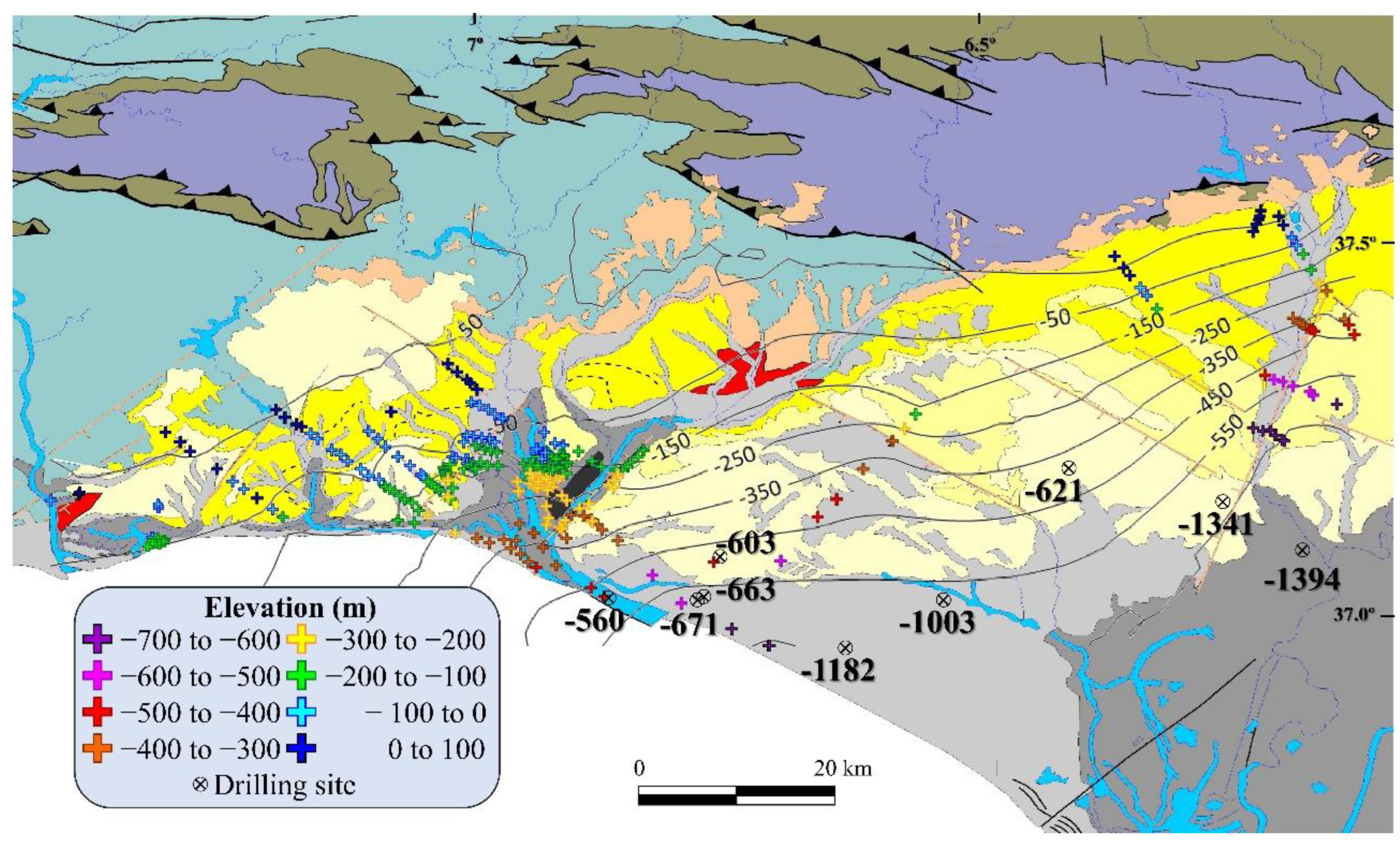
Figure 2. Elevation map over orthophotography (provided by the IGN), color-coded by range to highlight the slope on both margins of the two rivers.

Similarly, the Odiel River originates in the Sierra de Aracena and Picos de Aroche Natural Park (Huelva), flowing NW-SE through a narrow and steep valley until reaching the water reservoir “Embalse del Sancho”, located north of Gibraleón. From this point, the river adopts a N-S orientation, transitioning into an expansive marshland more than 4 km wide (designated as the Natural Area “Marismas del Odiel”) with gradients below 1% (see again Figure 2). The eastern margin of the Odiel is marked by prominent relief (up to 50 meters, locally known as “Cabezos de Huelva") with slopes occasionally exceeding 50%, while the western margin exhibits more subdued topography with elevations around 20 meters and slopes exceeding 10%.

Although less pronounced, the Piedras River also displays a reorientation in its final segment, adopting a well-defined NNE-SSW orientation over its last 12 km near the town of Lepe.

Special mention should be made of the numerous anthropogenic deposits and fills that cover the surface of the study area. Notably, immediately east of the city of Huelva, there is a massive phosphogypsum pond located directly on the marshlands, with dimensions nearly comparable to those of the city itself, which pose a significant environmental risk in the event of a plausible earthquake or tsunami. Additionally, the entire study area has been extensively used for agricultural purposes.

3. Methodology

The seismic noise recording in the Guadalquivir Basin was conducted in order to apply the Horizontal to Vertical Spectral Ratio (HVSR) method, which facilitates the identification of the soil fundamental frequency. This parameter is closely linked to the thickness of the sedimentary cover overlying a hard rock basement. The depth (h) of the mechanical discontinuity between the crystalline basement and the “soft” sedimentary cover is strongly correlated with the soil fundamental frequency (f₀) and the shear wave velocity (V_S) [37]. By applying an empirical equation, which relates the depth of the rock basement (not necessarily the geological Variscan basement) to the soil fundamental frequency, a three-dimensional map of the basin’s basement can be constructed.

Seismic noise measurements were carried out at a total of 334 discrete sampling points, many of which were integrated into profiles. Most of these profiles are oriented approximately NW-SE, following the general slope of the basement-cover contact (see Figure 3), with variable lengths ranging from 2 km to over 35 km. Additionally, orthogonal NE-SW profiles were designed to delineate potential structural features affecting the area.

The primary limitations encountered during this study were related to restricted access to protected areas, such as the “Marismas del Odiel” Natural Area (Huelva) and the Guadiamar Green Corridor (Seville), which limited vehicle entry and access to certain zones. However, efforts were made to maintain a sufficiently dense sampling grid in these areas to mitigate data gaps. Additional challenges included intense agricultural, industrial, and urban land use, which further restricted access to specific sites. Sampling efforts were consequently adapted to public areas, such as forest roads, walking paths, and other accessible zones.

This study includes seismic noise recordings acquired during the development of the ALERTES-RIM project, focusing on the central sampling area, specifically the city of Huelva and nearby industrial zones. Within this region, 5 seismic arrays were deployed in the city of Huelva to determine S-wave velocities (V_S), and 45 H/V sampling points were recorded, the results of which were previously published by the research team [17,19].

Additionally, this work incorporates data collected during six subsequent campaigns outside the scope of the ALERTES-RIM project and PGC2018-100914-B-I00, covering a total area exceeding 2,300 km² (see location in Figure 3).

Figure 3. Location of seismic noise sampling points in the western Guadalquivir basin.

The profiles were designed to ensure continuity in the seismic noise data, spanning from the boundary of the basin, where the Variscan basement (geological substratum) outcrops, towards the interior of the basin. This design facilitates the development of both surface and basement topographic profiles.

Some sampling points were positioned directly above historical deep exploratory boreholes, enabling the derivation of empirical relationships for calculating the depth of the basement rock [16,17]. Additional details on sampling, locations and other relevant information are provided in Table A1 of the annexes.

Seismic noise measurements were made with a SARA SL06 digitizer and a Lennartz LE 3D/5s triaxial seismometer, with a natural frequency of 0.2 Hz. Exceptionally, Lennartz LE-3D/20s, with natural frequency of 0.05 Hz were employed in areas presumed to have greater basement depths (southeastern portion of the study area). The equipment simultaneously recorded both time (UTC) and location through an integrated GPS device. The measurements used a sampling frequency of 200.

The minimum recording time was approximately 25–30 minutes, with a standard duration of 45 minutes per sampling session. Exceptionally, longer recording times (up to 90 minutes) were used in areas with adverse conditions, such as high background noise from vehicular traffic or greater substrate depths.

The recorded signal was processed using Geopsy (v. 3.4.2) [38], which generates graphs that relate the Fourier spectra of the horizontal components (N and E) to the vertical component (Z). This process yields an H/V vs. frequency graph from which the soil fundamental frequency (f₀) is determined. Between 7 and 19 calculation windows, each approximately 300 seconds long, were utilized for this analysis.

In most cases, the highest amplitude and lowest frequency peak in these graphs corresponds to the soil fundamental frequency. The high amplitude and narrow width of the peaks allowed for a precise determination of f₀.

The interpolation maps of basement depth were generated using Surfer (v. 15.6.3), employing kriging interpolation. These maps were subsequently imported into QGIS (v. 3.32), where they were overlaid onto the surface geological map.

4. Results and Interpretations

4.1. Empirical Equation for the Estimation of the Basement Depth from Vs and f0 for the Western Guadalquivir Basin

The soil fundamental frequency (f₀) is related to the shear wave velocity in the soft soil layer (V_S) and the thickness of this layer (h) following the relationship proposed by Bard [37] (1):

f_{0} = \frac{V_{S}}{4 h}

(1)

To calculate the depth of the bedrock (h), it is necessary to know the vertical profile of shear wave velocity (V_S) at each point where the fundamental frequency of the soil (f₀) has been measured. However, this information is often not available a priori. To address this issue, the vertical profile of V_S is parameterized using empirical relationships of the form h=a·f₀^b, derived from mechanical borehole or geophysical exploration data [5,39,40]. Evidently, the parameters a and b depend on the geomechanical characteristics of the materials constituting the soft soil layer.

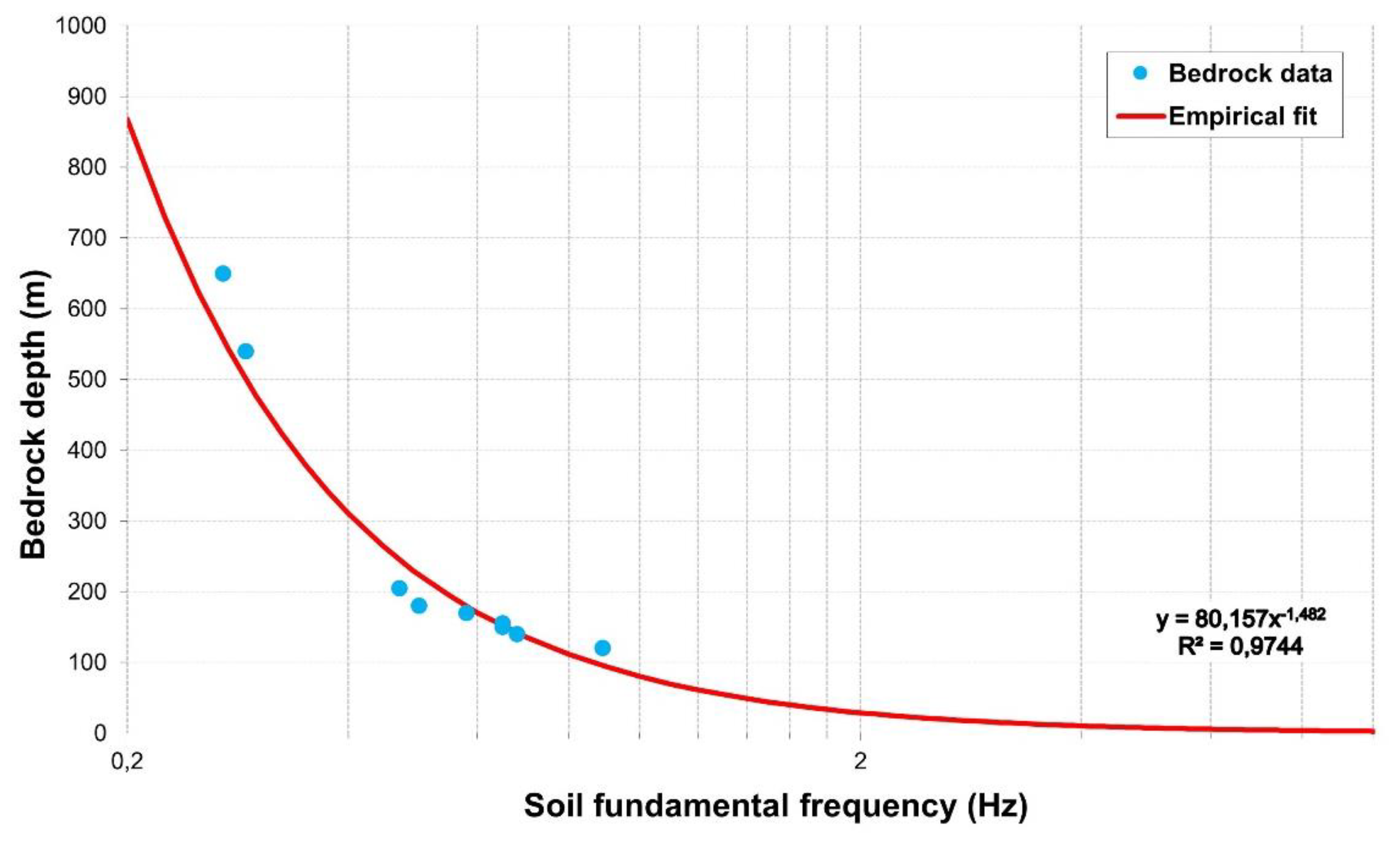
A new empirical relationship has been developed (Figure 4) for the southwestern region of the Guadalquivir Basin by combining data from the H/V spectral ratio method, array techniques (5 datasets), reflection seismics (2 datasets), and mechanical boreholes (2 datasets) that reached the bedrock. This empirical relationship was calibrated using nine data pairs, covering a frequency range from 0.27 to 0.89 Hz and a wide depth range from 120 to 650 meters. The correlation coefficient for this relationship is 97.44% (see Figure 4).

The equation used for estimating the depth is as follows (2):

h = 80.16 \cdot f_{0}^{- 1.48}

(2)

Figure 4. Empirical relationship for calculating the depth of the bedrock in the Guadalquivir Basin (near the city of Huelva) based on the fundamental frequency.

This differs slightly from the equation used in Alonso-Chaves et al. [19].

4.2. H/V Graphs, f0 and Estimated Basement Depth

Figure 5. Example of the five different responses obtained during the study. Dashed lines represent the measurement error, while continuous lines represent the average. The gray bands correspond to the uncertainty range in the calculation of f₀, where a wider band indicates greater indeterminacy in f₀. Finally, a peak is considered when its amplitude exceeds 2H/V.

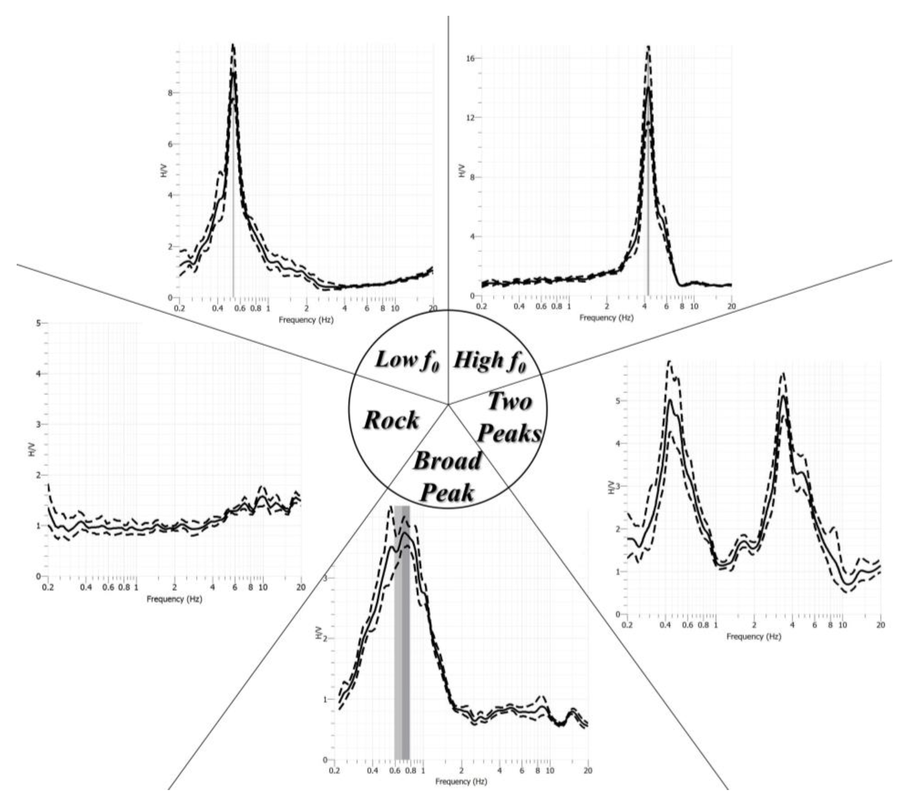
The analysis of 334 seismic noise sampling points has led to the conclusion that most of the H/V spectral ratio graphs exhibit high amplitude and a sufficiently defined peak width for accurate peak identification, with at least one peak exceeding 2 H/V (a necessary criterion for considering it as f₀). Furthermore, five distinct response types have been identified in the H/V spectral ratio (see Figure 5):

a): High-frequency H/V peaks (>1 Hz): Characteristic of areas where the bedrock is closer to the surface.
b): Low-frequency H/V peaks (<1 Hz): Indicative of deep-seated bedrock.
c): Broad peaks: Potentially associated with irregular bedrock surfaces, such as fault zones, which are critical areas for further study.
d): Multiple peaks (at least two exceeding 2 H/V): Typically found in marshlands or areas with significant lithological contrast between unconsolidated Quaternary sediments and other type of Neogene sediments.
e): Flat response (no peaks exceeding 2 H/V): Classified as "rock", characteristic of shallow or exposed bedrock.

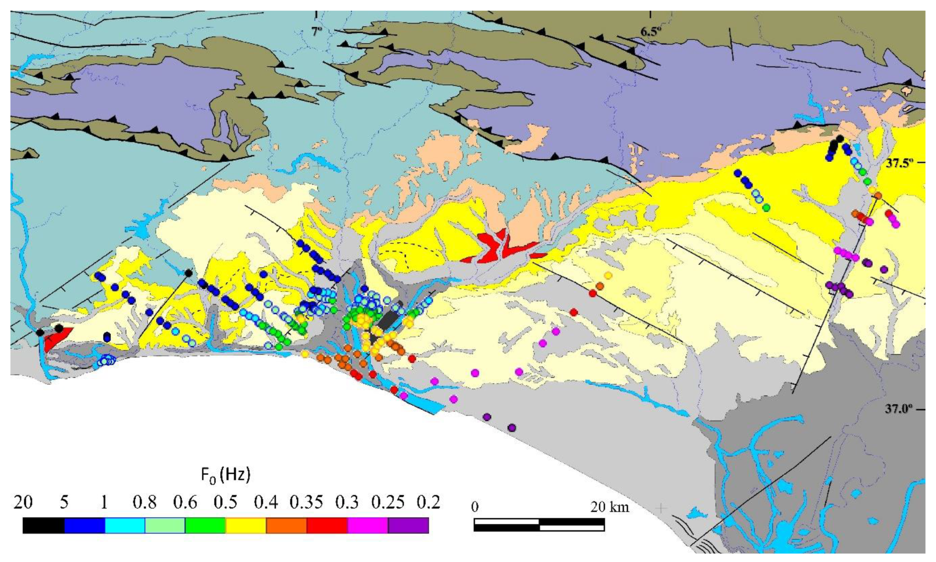
The fundamental frequency (f₀) estimated from these graphs ranges from 0.23 to 18 Hz, covering a wide spectrum of values (see Figure 6). The highest frequencies are systematically located near the basin margins (northern and northwestern areas), while lower frequencies dominate in the basin interior (southeastern areas). The f₀ values progressively decrease toward the SE, which correlates with the expected increase in sediment thickness and bedrock depth toward the basin interior (from NW to SE). Notably, the color bands representing different frequency ranges align closely with the structural boundary between the bedrock and sedimentary cover.

Figure 6. Fundamental frequency data measured with passive seismic over the same geological map of the study area (Figure 1). The colors represent different ranges of fundamental frequency: cold colors correspond to high frequencies, while warm colors indicate low fundamental frequencies.

Similarly, as shown in Figure 7, the flat response (rock-type, marked with a blue cross in the figure), observed at only one sampling point, is also located in the northwestern area, where the bedrock is either more exposed or even visible in certain sections.

Moreover, the areas where double-peak responses (green stars in Figure 7) are most concentrated are specifically located in marshlands and floodplains of various rivers. Wide peaks (yellow crosses in Figure 7) are systematically found along NE-SW oriented corridors near the Odiel River (on both the right and left banks) and NNE-SSW in the case of the Guadiamar River. As observed, these align with remarkable precision along fault traces identified through cartographic methods. However, no fault planes could be identified at the surface due to the unconsolidated nature of the overlying materials.

The basement depth is estimated to range from just a few meters below the surface level (or even outcropping in some areas) in the northern and northwestern parts of the study area to depths exceeding 600 meters, reaching up to -667 meters above the sea level in the southeasternmost sector (Figure 8).

The isolines corresponding to the mechanical basement elevation follow a fairly consistent N70-80ºE direction, aligning well with the morphology and orientation of the Guadalquivir Basin. However, deviations in orientation are observed near the rivers (Odiel, Tinto, and Guadiamar), where the isolines locally shift to an E-W direction, particularly beneath the city of Huelva, dipping southward. This pattern may be attributed to fractures affecting both the mechanical (and geological) basement and the overlying Neogene sediments.

Figure 7. Location of the different types of H/V spectral ratio responses vs. f₀ (examples of each response type are shown in Figure 5) in the westernmost sector of the Guadalquivir Basin, overlaid on the geological map of the area (Figure 1).

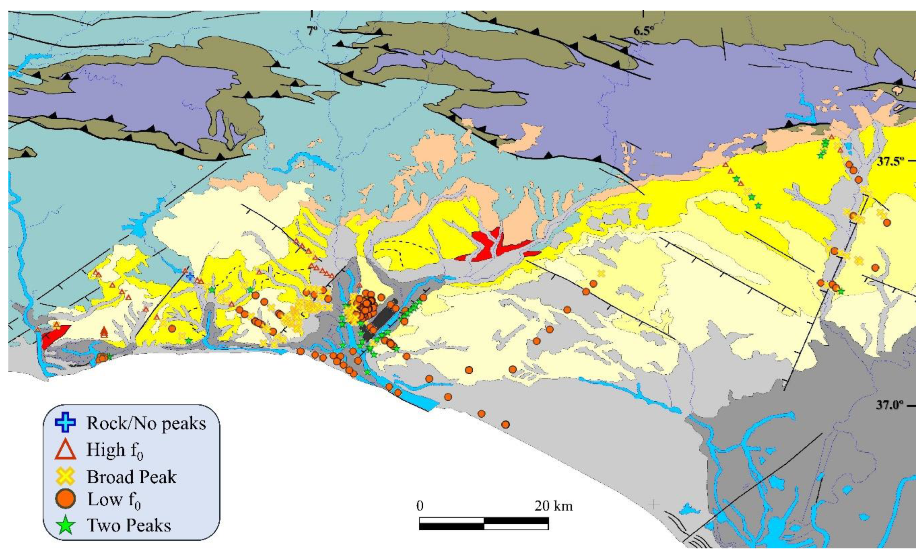
Figure 8. Map of basement depth (in meters above the sea level) estimated by kriging interpolation, based on depths obtained through the H/V method over the geological map (Figure 1). Faults in the study area have been smoothed to emphasize contour lines. Colored points represent depths derived from seismic noise measurements, while black points indicate depths obtained from borehole logging by IGME.

4.3. Profiles

Based on the transects conducted, most of which follow a NW-SE orientation and approximate the true dip of the mechanical basement, an average slope of approximately 1-3º dipping towards the SE has been estimated, with a standard deviation of around 1º. However, as seen in Figure 9, significant localized slope breaks of 5-7º have been identified. These slope discontinuities can be correlated across adjacent profiles (see Figure 9, also can be seen corresponding figures in Amador Luna et al. [20,21]). Notably, these ruptures tend to occur in areas near river channels.

In the Coast profile, three abrupt slope changes have been identified: two at the beginning of the Odiel marshes (on the western bank of the Odiel River, marked as b in Figure 9) and another at the confluence of the Odiel and Tinto rivers (c in the same figure). This subsurface morphology could explain the structural highs to the west and the depressed areas to the east (Odiel marshes and Huelva Estuary). The terraced morphology may be attributed to ancient river terraces on the western bank or to brittle structures (faults) that have downthrown the eastern sector.

Figure 9. Map showing the location of sampling points used to establish topographic and mechanical basement depth profiles. The lower section displays the profiles for each transect, with the red line representing the true-scale profile and the black line showing the vertically exaggerated scale (the vertical exaggeration is indicated in the lower right corner of each profile). Black and red points represent the estimated depth. On the right, the same profiles are presented with interpreted data: the dashed blue line represents the mechanical (non-geological) basement, while the dashed red line marks faults that may explain slope discontinuities. Additionally, the locations of various rivers and specific points of interest (labeled with letters) are indicated. The arrows with question marks indicate areas where the slope changes; however, further study would be required for a rigorous interpretation.

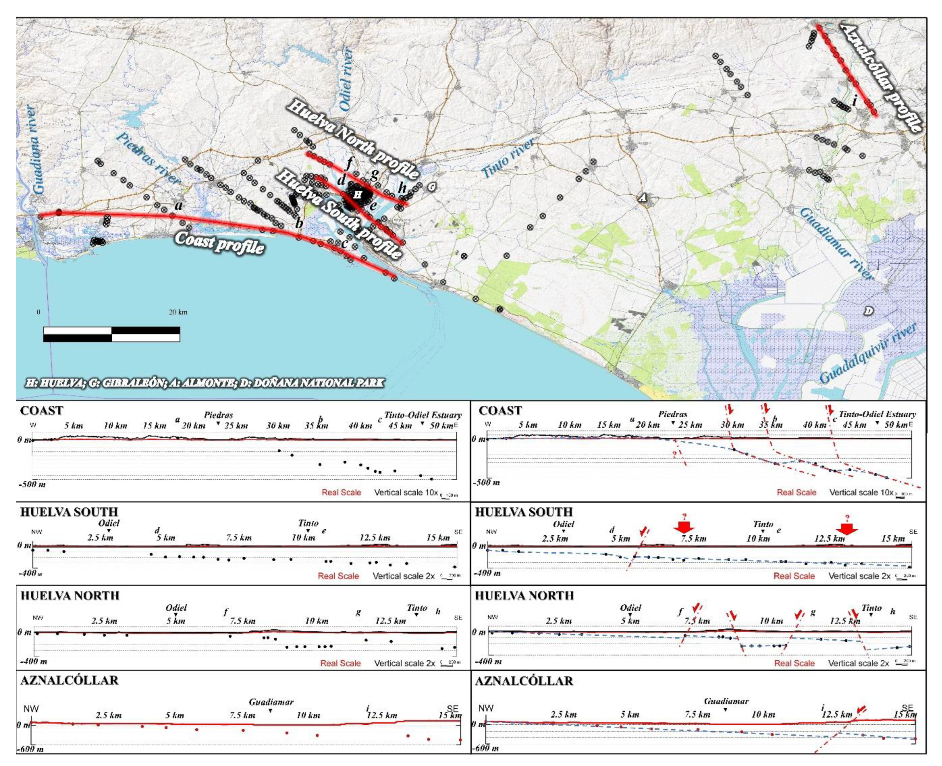
In the Huelva profiles, slope changes correlate well with known structural highs identified in the topographic profile, such as the Cabezos de Huelva, east of the Odiel (point d), and the Cabezos de Moguer and Palos, east of the Tinto River (only slightly visible east of the Huelva North profile). A slight elevation, corresponding to the location of northern part of the current phosphogypsum deposits is also observed just east of the city (g in the Huelva North profile).

Although the Huelva South profile requires further investigation in the areas marked with question marks in Figure 9, the slope changes show a very good correlation with the faults interpreted (and much more evident) in the Huelva North profile. Notably, the slope changes in both cases occur along corridors that can be correlated between the two profiles.

Another possibility is that the structures identified in the northern profile exhibit greater vertical displacements (several tens of meters) than those in the southern profile (a few tens of meters), making them more difficult to identify. A more detailed study at a smaller scale is planned in the future in order to better delineate these structures.

Across all cases, it is evident that sediment thickness remains minimal in the northwestern sector but increases markedly east of the Odiel River meridian, highlighting significant subsidence in the southeastern region.

In the Aznalcóllar area, the slope change becomes evident beyond the Guadiamar River, coinciding at the surface with an increase in topographic elevation. This could be explained by the presence of a fault that relatively uplifts the eastern block. Although no fault planes have been identified at the surface, the significant basement offset and the corresponding change in the eastern riverbank slope suggest the existence of an uplifted block.

In all cases, these slope discontinuities can be attributed to faults affecting both the mechanical (and geological) basement and the sedimentary cover. These faults are high-angle structures, extending over 8 to 15 km, with vertical displacements between 50 and 100 m, and can be correlated across different profiles, following NE-SW to NNE-SSW orientations.

5. Discussion

5.1. Geology and Passive Seismic Results

As shown in Figure 6 to Figure 9, the results from passive seismic methods are highly consistent with surface geology and the depth estimations inferred from it. High-frequency signals (indicating shallower basement depths) are systematically located near the boundary between the basement and the sedimentary basin, progressively deepening toward the southeast, as expected. Conversely, low-frequency signals (indicating deeper basement levels) are concentrated in the southeastern areas (near to Mazagón or Villamanrique de la Condesa surroundings). The primary orientation of the isolines also exhibits a strong parallelism with this boundary, following an N60–80ºE trend. Changes in the basement slope direction coincide with the river channels and variations in surface topography, aligning with the mapped fault traces. However, no fault planes have been identified at the surface. Due to the lithological characteristics of the area—dominated by expansive clays—the identification of fault planes in the field becomes particularly challenging. These materials are prone to intense weathering and plastic deformation, which tend to obscure or entirely erase the structural evidence typically associated with fault planes. As a result, surface expressions of tectonic structures are often subtle or absent, making direct observation and mapping of fault planes virtually impossible without geomorphological criteria or geophysical or subsurface data.

The cross-sections reveal significant changes in the deep basement slope, which also correlate with geomorphological features and mapped fault traces. These vertical separations are estimated to range between 50 and 100 meters, affecting both the basement and its overlying cover, which may explain certain cartographic features. These slope variations can be correlated across different profiles, exhibiting an approximate N70–80ºE (or even NNE–SSW) orientation, once again coinciding with the basin’s main structural trend.

Two main interpretations can be proposed for these slope changes: (i) they may correspond to ancient fluvial terraces of the Guadalquivir River, which has migrated eastward since the Miocene, leaving elevated terraces in the westernmost part of the basin; or (ii) they may be associated with fractures that control both surface relief and river courses. If the latter is the case, these fractures align well with the passive seismic records, where broad spectral peaks have been observed, typically associated with irregular basement structures such as fault zones. These alignments are consistent with previous studies [19,41]. Therefore, these slope discontinuities can be attributed to faults affecting both the mechanical (and geological) basement and the sedimentary cover. These faults are high-angle structures, extending over 8 to 15 km, with vertical displacements between 50 and 100 m, and can be correlated across different profiles NE-SW to NNE-SSW. A possible interpretation of these slope variations along the cross-sections as faults is illustrated in Figure 9 (right), where many of these fractures can be correlated across different profiles.

Three main fault zones have been identified in the western part: one at the easternmost end of the Odiel River (coinciding with the relief of the Cabezos de Huelva, see d and f in Figure 9), another at its western margin (see b in Figure 9), and a third one along the eastern margin of the Tinto River near Moguer. Additionally, another fault may be present along the eastern margin of the Guadiamar River. In the central sector of the study area, particularly near Almonte, a noticeable curvature in the orientation of the isolines is observed. This feature coincides with changes in lithology and topographic forms, suggesting the possible presence of a fault, although its fault plane is not identifiable in the field. The so-called “Almonte Fault” and its surrounding areas will be the subject of future investigations, aimed at identifying additional fault structures inferred from satellite imagery, even if their fault planes remain untraceable on the ground.

Figure 2 further reveals a sharp topographic break in southern Huelva. The orientation of this possible structure is also reflected in one of the western branches of the Odiel River, and if extended eastward, it coincides with the phosphogypsum deposits. This WNW–ESE-trending structure can also be identified in seismic records, where broad spectral peaks align in the same direction. Moreover, Figure 2 shows that the elevation of the phosphogypsum deposits in the northern sector (>30 m) is higher than in the southern sector (where maximum elevations are around 20 m), potentially indicating subsidence of the southern block, consistent with a south-dipping normal fault. These observations are in agreement with previous studies by González [42] and represent a significant environmental risk due to the critical location of these deposits above a structural feature. This feature can be inferred from not only by digital imagery (as shown in Figure 2), deduced from changes in the orientation of the isolines in Figure 8, and even identified in the seismic profiles in Figure 9 (point e).

5.2. Boreholes

Some of the passive seismic measurements, as shown in Figure 8, were conducted directly above historical boreholes drilled by the IGME and oil companies. These measurements aimed to compare the depth estimates obtained through the passive seismic method with those derived from borehole data.

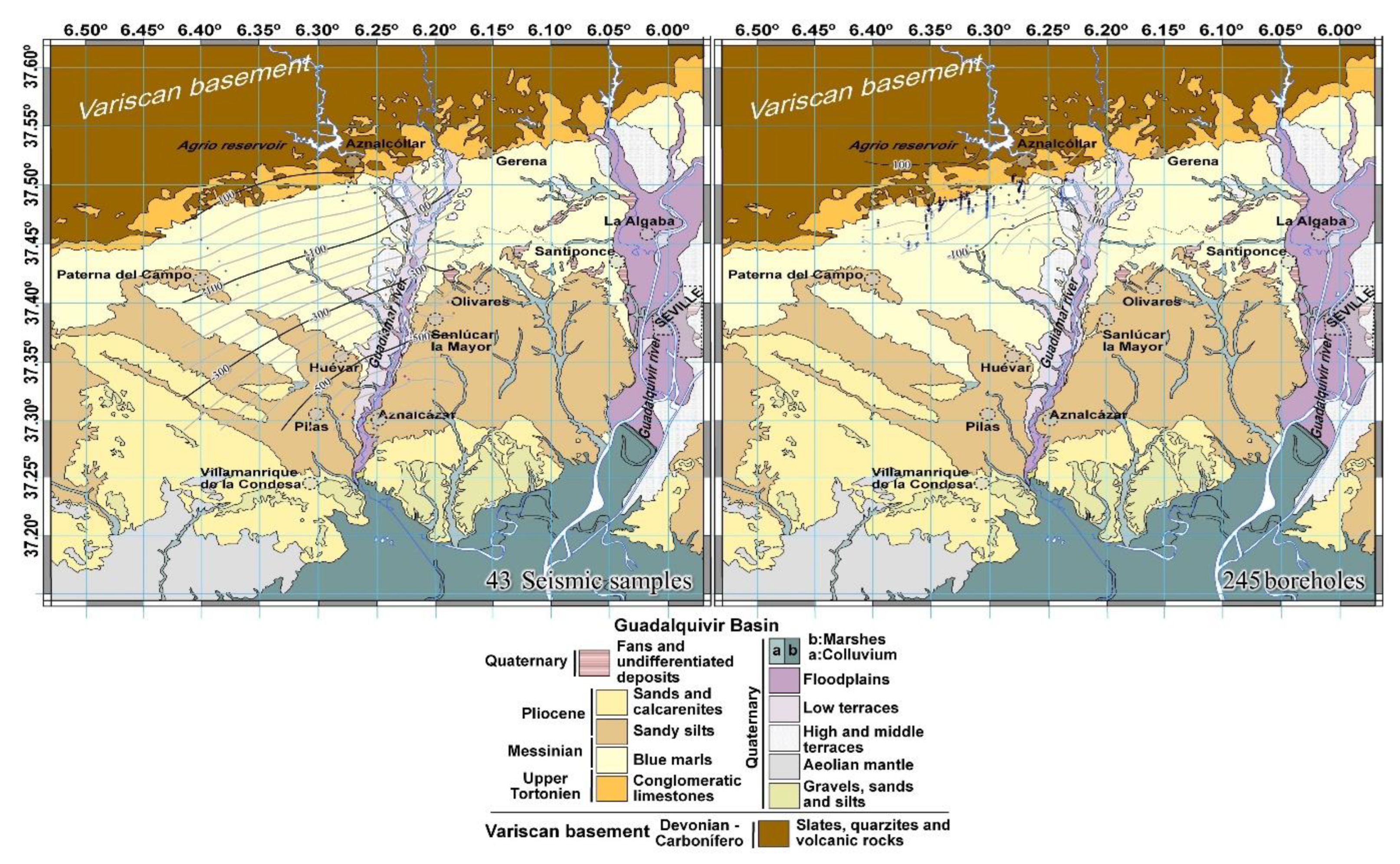
Saltés-1, the easternmost borehole, reached the geological basement at an elevation of -560 m (meters above the sea level), while the passive seismic sampling point HU42, located vertically above it, estimated a mechanical basement depth of -494 m. In the case of Huelva-1, which reached -603 m for the geological basement, HU41 estimated a depth of -500 m for the geological basement. Lastly, the Moguer-1 and Mazagón-1 boreholes reached the basement at -679 m, whereas HVAME16 estimated a mechanical basement depth of -585 m. For the Aznalcóllar case, a similar pattern was observed, with an estimated depth discrepancy of approximately 30–50 meters above the actual geological basement depth (see Figure 10). As previously mentioned, this discrepancy may be attributed to the Niebla calcarenites, which outcrop in the northern part of the study area and have been confirmed to extend in depth through borehole data [18]. This formation, although it is part of the basin filling, behaves as a mechanically rigid substrate, contrasting with the softer basin sediments. The observed 30-meter error in the northern zone and the approximately 100-meter discrepancy further into the basin could be related to the increasing thickness of this material toward the basin interior, with the actual geological basement lying between 30 and 100 meters below the estimated mechanical basement.

A separate discussion is warranted for boreholes located deeper within the basin, where geological basement depths exceed -1000 m. The passive seismic method typically operates at frequencies ranging from 0.2 to 20 Hz, corresponding to a maximum depth of approximately 850 meters (based on empirical formula). Thus, at such depths, the method could not reach the mechanical basement. However, in a nearby area, as shown in Figure 8, a well-defined depth of approximately -660 m has been identified (see ARNO in Table A1 in appendix). This suggests the presence of a fault with significant throw toward the southeast, which could explain the substantial depth variation between these points.

Lastly, the Almonte-1 borehole, located further north, reached the geological basement at approximately -620 m—significantly deeper than the depth estimated by the seismic method. However, this borehole is situated between two fault systems identified in geological mapping, which correspond well with changes in the curvature of the depth isolines and are referenced by only a few nearby data points. This region is of particular interest, as borehole data indicate a former structural high (characterized by a thinner sedimentary cover compared to adjacent boreholes and the absence of certain units, such as the Guadalquivir sands). This elevated structure, along with those identified along the eastern margin of the Guadiamar and the western margin of the Guadalquivir, may represent active tectonic features that could have influenced the Guadalquivir River course and its progressive eastward migration. The presence of olistostrome bodies in boreholes further east from the study area (Villamanrique de la Condesa to the south) also suggests that the Miocene orogenic front was previously located further west, with the Guadalquivir Basin shifting over time. Future surveys should aim to increase data density in this area and extend measurements toward the Guadalquivir to enhance the depth model.

A similar approach was later applied in the Aznalcóllar area using boreholes provided by various companies operating in the area (see Figure 10), revealing a similar pattern with minor discrepancy —of around 30 meters—between HVSR-derived estimates and borehole measurements.

Figure 10. Comparison of depth maps (generated through kriging interpolation) between passive seismic data (left) and exploration borehole data (right).

5.3. 3-D Architecture

Figure 11. Composite figure of satellite image (top), geological map with data derived from interpolation of seismic noise measurements (Figure 45, middle), and 3D model derived from these data (bottom) of the westernmost sector of the Guadalquivir Basin.

The morphology of the mechanical basement in the westernmost sector of the Guadalquivir Basin (considering that the Variscan basement should be located a few tens meters below it) is illustrated in Figure 11.

As shown, the interpretations derived from all observations align well with the surface morphology and geology, presenting a general slope towards the southeast, from very shallow or even outcropping basement materials in the west, to deep basements in the east (depths greater than 600 m). Sudden changes in slope are systematically located along the riverbeds, aligning approximately in NE-SW directions (Piedras, Odiel, and Tinto rivers) or NNE-SSW directions (Guadiamar).

In summary, the relief of the western end of the Guadalquivir basin can be explained by the development of structures that create a horst and graben landscape, with the horsts located in areas such as the Cabezos de Huelva and other topographically higher zones (as can be also in the eastern end of the Guadiamar), and the grabens being associated with the river marshes. These structures could be explained by the accommodation of deformation caused by the advance of the Alpine orogenic front (the Betics) in the forebulge region, significantly distanced from the front itself.

6. Conclusions

Seismic noise measurements were conducted at 334 discrete sampling points in the southwestern end of the Guadalquivir Basin to apply the Horizontal-to-Vertical Spectral Ratio (HVSR) method. The data presented in this study indicate that both the geological and mechanical basement are aligned along an azimuth of N070ºE and exhibit a gentle southeastward dip, oriented toward the Alpine orogenic front. This structural surface is disrupted by north-trending fault systems. The integration of 334 data points distributed over an area slightly exceeding 2300 km² has enabled the construction of a three-dimensional model that delineates first-order reference surfaces relevant to basin architecture— such as, conceptually, the sedimentary fill interface or basin wall.

Furthermore, the incorporation of seismic noise data along NW-SE-oriented profiles permits the identification of variations in the dip of the mechanical basement in two-dimensional cross-sections. Borehole data suggest that similar structural variations may also be present in the geological basement, providing additional support for the observed subsurface heterogeneities.

A new empirical relationship was developed for the southwestern Guadalquivir Basin by integrating data from the HVSR method, seismic array techniques (5 datasets), reflection seismics (2 datasets), and mechanical boreholes (2 datasets) that reached the bedrock. This relationship, expressed as h=80.16·f₀^-1.48, enabled the determination of the mechanical basement depth, the Tortonian paleotopography, and the presence of potential fractures influencing current topography.

The geological basement reaches depths exceeding 600 m near Mazagón and Villamanrique de la Condesa, located in the southeastern part of the study area. The estimated dip of the basement surface is approximately 1–3º southeastward, with slope breaks coinciding with fluvial courses. The main structural trend follows a N070ºE orientation, aligning with the basement-cover contact.

The HVSR spectral ratio method yielded five distinct response types: (i) high-frequency peaks or (ii) no response, associated with shallow or outcropping basement in the northwestern sector; (iii) low-frequency peaks in the southeastern sector, indicative of deep-seated basement; (iv) double peaks in marshland areas; and (v) broad peaks, characteristic of irregular basement surfaces, potentially corresponding to fault zones.

The presence of sites exhibiting at least two peaks in the H/V spectral ratio may reflect not only contrasts in the mechanical behavior of the materials composing the subsurface at those locations, but also potential lithological changes. These double peaks could indicate the presence of different materials within the basin fill itself. As such, the detailed analysis of these features warrants particular attention in future investigations.

Passive seismic results show strong consistency with surface geological observations and depth estimations. Borehole data validated these depth estimations, with minor discrepancies ranging from 30 to 100 m, likely due to the presence of mechanically rigid units such as the Niebla calcarenites.

Two main hypotheses are proposed to explain abrupt slope changes: (i) they may represent ancient fluvial terraces formed by the eastward migration of the Guadalquivir River since the Miocene, or (ii) they may be related to fault activity controlling surface

relief including the orientation and flow direction of rivers. The alignment of broad seismic peaks with mapped fault zones supports the latter hypothesis, suggesting active or reactivated fault structures.

At depths greater than 800 m, the HVSR method presents limitations; however, the strong variations in basement depth suggest significant faulting in the southeastern sector of the study area.

The interpreted basement morphology reveals a horst and graben system, with structural highs corresponding to elevated areas (e.g., to the west of the Odiel estuary, Cabezos de Huelva, east of the Tinto estuary, or in the Aljarafe area in Seville) and depressions associated with river marshes in the northern margin of the Gulf of Cadiz, including the marshes of Odiel, Tinto and Doñana, among others.

The observed structural configuration is likely attributable to lithospheric flexure, facilitating upper-crustal extension. This tectonic regime is consistent with deformation expected in a forebulge setting, associated with the northern segment of the Gibraltar Arc in response to the propagation of the Alpine orogenic front.

Given the structural complexity of the western Guadalquivir Basin, future research should focus on increasing data density, particularly in northeastern areas where borehole data indicate structural highs or anomalies. Additional passive seismic surveys, complemented by geophysical techniques and detailed geological mapping, will be essential to refine the depth model and improve understanding of the tectonic evolution of the region.

Moreover, the methodology developed in this study opens new avenues for research across various branches of Earth Sciences. In particular, it shows strong potential for application in hydrocarbon exploration, where it could serve as a preliminary tool for identifying potential structural traps and fault systems, including blind faults. Notably, the Cobre Las Cruces deposit—one of the most significant copper deposits globally—was discovered within the study area, beneath the sedimentary fill of the Guadalquivir Basin and rooted in the Variscan basement. This technique could therefore prove highly usefull in the identification of similar new buried mineral deposits.

Geophysical anomalies, including gravimetric data, combined with the application of the H/V spectral ratio technique, may offer an effective approach for delineating the geometry of sedimentary fills that overlie geologically prospective zones. Additionally, the areas provide valuable input for seismic vulnerability assessments of infrastructure. This is particularly relevant in seismically active regions such as the San Vicente Transpressive Zone (see [43]), where the occurrence of high-magnitude earthquakes remains a plausible scenario.

To sum up, the generation of three-dimensional maps of the bedrock surface, the recognition of blind faults, along with the determination of soil fundamental frequencies, would enable the development of more detailed hazard maps in areas of high seismic and tsunamigenic risk—such as the study area. Given its simplicity, versatility, rapid data acquisition, low cost, and reliable results, this technique has the potential to become a powerful tool across a range of applications. While its utility in geological studies is demonstrated in the present work, it also holds significant promise for other fields such as civil engineering, geotechnics, hydrocarbon industries and even mining.

Acknowledgments

David Amador Luna acknowledges the funding from the ‘Estrategia Política de Investigación y Transferencia’ (EPIT) of the University of Huelva for the predoctoral contract to promote the hiring of novice research personnel (EPIT20/00832), without which this work would not have been possible. We also would like to thank to ALERTES-RIM and “Analisis Multidisciplinar y multiescala de los mecanismos de localización y reparto de la deformación cortical en convergencia oblicua”, PGC2018-100914-B-I00, this study includes seismic noise recordings acquired during the development of these projects.

Appendix A

Appendix A.1

Table A1. Summary table of the measurements conducted in the Guadalquivir Basin, including coordinates, fundamental frequency, estimated thickness, basement depth, and interpretation of the resulting HVSR curves.

STATION	COORDINATES		FUNDAMENTAL FREQUENCY (f₀) (Hz)	THICKNESS (m)	ELEVATION (m)	INTERPRETATION
STATION	LAT (°)	LONG (°)	FUNDAMENTAL FREQUENCY (f₀) (Hz)	THICKNESS (m)	ELEVATION (m)	INTERPRETATION
HVAME2	37.2888	-6.9326	0.74	125	-84	LOW F₀ PEAK
HVAME3	37.2859	-6.9255	0.77	118	-79	LOW F₀ PEAK
HVAME4	37.2817	-6.9108	0.71	133	-106	LOW F₀ PEAK
HVAME10	37.2265	-6.9096	0.43	280	-276	TWO PEAKS
HVAME11	37.2202	-6.9057	0.38	336	-321	LOW F₀ PEAK
HVAME12	37.2171	-6.8987	0.37	349	-311	LOW F₀ PEAK
HVAME13	37.1654	-6.8418	0.28	527	-506	LOW F₀ PEAK
HVAME14	37.2121	-6.8932	0.36	364	-345	LOW F₀ PEAK
HVAME15	37.2151	-6.8977	0.38	336	-298	LOW F₀ PEAK
HVAME5	37.2714	-6.8980	0.7	136	-127	LOW F₀ PEAK
HVAME7	37.2391	-6.9268	0.47	245	-241	LOW F₀ PEAK
HVAME8	37.2347	-6.9225	0.46	253	-246	LOW F₀ PEAK
HVAME9	37.2472	-6.9346	0.5	224	-222	BROAD PEAK
HVAME16	37.1391	-6.8149	0.25	624	-585	LOW F₀ PEAK
HVAME17	37.1975	-6.8746	0.33	414	-382	LOW F₀ PEAK
HVAME18	37.2079	-6.8889	0.39	323	-319	TWO PEAKS
HVAME19	37.3162	-6.5948	0.44	270	-159	BROAD PEAK
HVAME20	37.3021	-6.6058	0.37	349	-246	LOW F₀ PEAK
HVAME21	37.2910	-6.6163	0.33	414	-316	LOW F₀ PEAK
HVAME22	37.2639	-6.6438	0.3	476	-376	LOW F₀ PEAK
HVAME23	37.2365	-6.6689	0.29	501	-413	LOW F₀ PEAK
HVAME24	37.2894	-7.0182	0.83	106	-74	LOW F₀ PEAK
HVAME25	37.2861	-7.0071	0.75	123	-114	LOW F₀ PEAK
HVAME26	37.2832	-6.9984	0.71	133	-120	BROAD PEAK
HVAME27	37.2820	-6.9937	0.62	163	-156	BROAD PEAK
HVAME28	37.1143	-6.7674	0.24	663	-619	LOW F₀ PEAK
HVAME29	37.1781	-6.7219	0.27	557	-512	LOW F₀ PEAK
HVAME30	37.2195	-6.6871	0.29	501	-429	LOW F₀ PEAK
HVAME31	37.2664	-7.0064	0.76	120	-116	BROAD PEAK
HVAME32	37.2737	-7.0145	0.89	95	-91	BROAD PEAK
HVAME33	37.2755	-7.0293	1.35	51	-46	BROAD PEAK
HVAME34	37.2640	-7.0180	0.68	142	-132	BROAD PEAK
HVAME35	37.2680	-6.9864	0.56	189	-187	BROAD PEAK
HVAME36	37.2679	-6.9968	0.69	139	-136	BROAD PEAK
HVAME37	37.2702	-7.0029	0.8	112	-109	BROAD PEAK
HVAME38	37.2804	-6.9873	0.58	180	-174	LOW F₀ PEAK
HVAME39	37.1533	-6.8994	0.31	454	-451	LOW F₀ PEAK
HVAME40	37.1746	-6.9311	0.34	396	-393	TWO PEAKS
HVAME41	37.2049	-6.9522	0.38	336	-331	LOW F₀ PEAK
HVAME42	37.1915	-6.9443	0.36	364	-361	LOW F₀ PEAK
HVAME43	37.2134	-6.9660	0.39	323	-320	TWO PEAKS
HVAME44	37.2530	-6.9677	0.52	211	-207	TWO PEAKS
HVAME45	37.2257	-7.0604	0.56	189	-159	BROAD PEAK
HVAME46	37.2218	-7.0524	0.5	224	-211	BROAD PEAK
HVAME47	37.1989	-6.9804	0.37	349	-345	LOW F₀ PEAK
HVAME48	37.1973	-6.9692	0.38	336	-331	LOW F₀ PEAK
HVAME49	37.1724	-6.9509	0.33	414	-410	LOW F₀ PEAK
HVAME50	37.1849	-6.9655	0.36	364	-359	LOW F₀ PEAK
HVAME51	37.2985	-6.9427	1.17	64	-62	HIGH F₀ PEAK
HVAME52	37.2329	-7.0664	0.58	180	-155	LOW F₀ PEAK
HVAME53	37.2434	-7.0832	0.55	194	-156	LOW F₀ PEAK
HVAME54	37.1952	-6.9947	0.39	323	-317	LOW F₀ PEAK
HVAME55	37.1897	-6.9749	0.36	364	-359	LOW F₀ PEAK
HVAME56	37.2584	-7.1073	0.93	89	-32	LOW F₀ PEAK
HVAME57	37.2640	-7.1146	0.83	106	-46	LOW F₀ PEAK
HVAME58	37.2046	-7.0267	0.42	289	-281	LOW F₀ PEAK
HVAME59	37.2719	-7.1266	1.38	50	-32	HIGH F₀ PEAK
HVAME60	37.2784	-7.1339	1.51	44	-20	BROAD PEAK
HVAME61	37.2975	-7.1619	1.69	37	-22	BROAD PEAK
HVAME62	37.3038	-7.1705	8.55	3	20	HIGH F₀ PEAK
HVAME63	37.3060	-7.1755	4.05	10	23	HIGH F₀ PEAK
HVAME64	37.3124	-7.1861	-	-	33	ROCK
HVAME65	37.3194	-7.1936	5.39	7	56	HIGH F₀ PEAK
HVAME66	37.3178	-7.0867	1.59	40	16	HIGH F₀ PEAK
HVAME67	37.2663	-6.8902	0.62	163	-152	LOW F₀ PEAK
HVAME68	37.2489	-7.0930	0.65	152	-120	LOW F₀ PEAK
HVAME69	37.2553	-7.0979	0.81	109	-69	BROAD PEAK
HVAME70	37.2824	-7.1416	1.5	44	-18	BROAD PEAK
HVAME71	37.2924	-7.1550	1.37	50	-25	TWO PEAKS
HU1	37.2746	-6.9403	0.62	163	-98	LOW F₀ PEAK
HU2	37.2725	-6.9404	0.6	171	-123	LOW F₀ PEAK
HU3	37.2779	-6.9464	0.77	118	-97	BROAD PEAK
HU4	37.2739	-6.9535	0.76	120	-117	LOW F₀ PEAK
HU5	37.2693	-6.9621	0.66	148	-146	TWO PEAKS
HU6	37.2502	-6.9436	0.5	224	-223	BROAD PEAK
HU7	37.2709	-6.9254	0.67	145	-125	LOW F₀ PEAK
HU8	37.2793	-6.9386	0.65	152	-102	INDETERMINED
HU9	37.2764	-6.9361	0.66	148	-108	LOW F₀ PEAK
HU10	37.2717	-6.9332	0.62	163	-132	LOW F₀ PEAK
HU11	37.2735	-6.9306	0.66	148	-119	LOW F₀ PEAK
HU12	37.2787	-6.9506	0,86	100	-95	BROAD PEAK
HU13	37.2758	-6.9498	0.81	109	-103	BROAD PEAK
HU14	37.2684	-6.9552	0.67	145	-141	TWO PEAKS
HU15	37.2602	-6.9601	0.55	194	-190	BROAD PEAK
HU16	37.2549	-6.9579	0.55	194	-190	TWO PEAKS
HU17	37.2607	-6.9272	0.54	200	-193	LOW F₀ PEAK
HU18	37.2577	-6.9253	0.52	211	-205	LOW F₀ PEAK
HU19	37.2605	-6.9227	0.55	194	-188	LOW F₀ PEAK
HU20	37.2561	-6.9302	0.5	224	-216	LOW F₀ PEAK
HU21	37.2535	-6.9351	0.47	245	-235	LOW F₀ PEAK
HU22	37.2522	-6.9380	0.46	253	-249	LOW F₀ PEAK
HU23	37.2583	-6.9358	0.48	238	-222	LOW F₀ PEAK
HU24	37.2599	-6.9385	0.48	238	-219	LOW F₀ PEAK
HU25	37.2664	-6.9390	0.53	205	-173	LOW F₀ PEAK
HU26	37.2639	-6.9393	0.5	224	-194	LOW F₀ PEAK
HU27	37.2693	-6.9302	0.61	167	-141	LOW F₀ PEAK
HU28	37.2674	-6.9462	0.53	205	-158	LOW F₀ PEAK
HU29	37.2742	-6.9454	0.61	167	-100	LOW F₀ PEAK
HU30	37.2649	-6.9512	0.53	205	-198	LOW F₀ PEAK
HU31	37.2624	-6.9457	0,5	224	-184	LOW F₀ PEAK
HU32	37.2605	-6.9452	0.49	230	-196	LOW F₀ PEAK
HU33	37.2513	-6.9567	0.48	238	-235	BROAD PEAK
HU34	37.2642	-6.9582	0.54	200	-197	BROAD PEAK
HU35	37.2811	-6.9412	0.71	133	-106	BROAD PEAK
HU36	37.2784	-6.9280	0.69	139	-106	LOW F₀ PEAK
HU37	37.2619	-6.9474	0.5	224	-191	LOW F₀ PEAK
HU38	37.2578	-6.9469	0.48	238	-199	BROAD PEAK
HU39	37.2578	-6.9489	0.48	238	-212	LOW F₀ PEAK
HU40	37.1774	-6.7842	0.27	557	-500	LOW F₀ PEAK
HU41	37.1774	-6.7842	0.27	557	-500	LOW F₀ PEAK
HU42	37.1446	-6.8867	0.29	501	-494	LOW F₀ PEAK
G9-10 HU3	37.2440	-6.9662	0.5	224	-222	TWO PEAKS
G25-26 HU3	37.2439	-6.9667	0.48	238	-236	TWO PEAKS
G40 HU3	37.2439	-6.9671	0.5	224	-222	TWO PEAKS
R0S1	37.2503	-6.9504	0.44	270	-266	TWO PEAKS
R1S2	37.2504	-6.9506	0.46	253	-249	TWO PEAKS
R1S3	37.2505	-6.9502	0.47	245	-241	TWO PEAKS
R1S4	37.2501	-6.9503	0.46	253	-249	TWO PEAKS
R2S5	37.2507	-6.9505	0.38	336	-331	LOW F₀ PEAK
R2S6	37.2502	-6.9498	0.47	245	-241	TWO PEAKS
R2S7	37.2500	-6.9507	0.47	245	-241	LOW F₀ PEAK
R3S2	37.2507	-6.9514	0.48	238	-234	LOW F₀ PEAK
R3S3	37.2509	-6.9495	0.46	253	-249	LOW F₀ PEAK
R3S4	37.2494	-6.9501	0.47	245	-240	LOW F₀ PEAK
R4S5	37.2523	-6.9514	0.49	230	-227	LOW F₀ PEAK
R4S6	37.2496	-6.9479	0.47	245	-241	LOW F₀ PEAK
R4S7	37.2488	-6.9528	0.48	238	-234	LOW F₀ PEAK
R5S2	37.2505	-6.9547	0.44	270	-266	BROAD PEAK
R5S3	37.2528	-6.9474	0.43	280	-275	BROAD PEAK
R5S4	37.2467	-6.9494	0.48	238	-234	BROAD PEAK
R0S1	37.2696	-6.9232	0.64	155	-140	LOW F₀ PEAK
R1S2	37.2696	-6.9230	0.65	152	-137	LOW F₀ PEAK
R1S3	37.2698	-6.9233	0.66	148	-133	LOW F₀ PEAK
R1S4	37.2695	-6.9235	0.66	148	-133	LOW F₀ PEAK
R2S5	37.2699	-6.9228	0.65	152	-137	LOW F₀ PEAK
R2S6	37.2697	-6.9238	0.64	155	-139	LOW F₀ PEAK
R2S7	37.2692	-6.9231	0.64	155	-140	LOW F₀ PEAK
R3S2	37.2694	-6.9221	0.64	155	-141	LOW F₀ PEAK
R3S3	37.2705	-6.9234	0.66	148	-132	LOW F₀ PEAK
R3S4	37.2691	-6.9241	0.64	155	-139	LOW F₀ PEAK
R4S5	37.2711	-6.9214	0.67	145	-131	LOW F₀ PEAK
R4S6	37.2703	-6.9259	0.64	155	-134	LOW F₀ PEAK
R4S7	37.2673	-6.9226	0.63	159	-146	LOW F₀ PEAK
R0S1	37.2659	-6.9295	0.58	180	-163	LOW F₀ PEAK
R1S2	37.2660	-6.9292	0.57	184	-167	LOW F₀ PEAK
R1S3	37.2661	-6.9297	0.58	180	-162	LOW F₀ PEAK
R1S4	37.2657	-6.9295	0.57	184	-168	LOW F₀ PEAK
R2S5	37.2664	-6.9294	0.58	180	-161	LOW F₀ PEAK
R2S6	37.2656	-6.9292	0.58	180	-164	LOW F₀ PEAK
R2S7	37.2658	-6.9300	0.58	180	-164	LOW F₀ PEAK
R3S2	37.2662	-6.9284	0.58	180	-163	LOW F₀ PEAK
R3S3	37.2665	-6.9303	0.58	180	-161	LOW F₀ PEAK
R3S4	37.2650	-6.9299	0.56	189	-175	LOW F₀ PEAK
R0S1	37.2775	-6.9251	0.68	142	-122	LOW F₀ PEAK
R1S2	37.2776	-6.9248	0.68	142	-122	LOW F₀ PEAK
R1S3	37.2776	-6.9253	0.68	142	-121	LOW F₀ PEAK
R1S4	37.2772	-6.9251	0.69	139	-119	LOW F₀ PEAK
R2S5	37.2779	-6.9250	0.68	142	-121	LOW F₀ PEAK
R2S6	37.2772	-6.9247	0.69	139	-120	LOW F₀ PEAK
R2S7	37.2773	-6.9257	0.68	142	-118	LOW F₀ PEAK
HU43	37.2898	-6.9889	0.83	106	-93	BROAD PEAK
HU44	37.2928	-6.9943	0.97	84	-68	LOW F₀ PEAK
HU46	37.2935	-7.0013	0.95	86	-68	BROAD PEAK
HU47	37.2951	-7.0085	1.06	74	-51	BROAD PEAK
HU48	37.2956	-7.0154	1	80	-67	BROAD PEAK
HU49	37.2680	-6.9497	0.55	194	-180	BROAD PEAK
HU50	37.2597	-6.9552	0.53	205	-202	BROAD PEAK
HU51	37.2629	-6.9345	0.52	211	-187	LOW F₀ PEAK
HU52	37.2562	-6.9539	0.5	224	-218	BROAD PEAK
HU53	37.2547	-6.9406	0.46	253	-239	LOW F₀ PEAK
HU54	37.2566	-6.9470	0.48	238	-228	LOW F₀ PEAK
Odiel1	37.2837	-6.9497	0.88	97	-95	BROAD PEAK/TWO PEAKS
Odiel2	37.2836	-6.9501	0.91	92	-90	BROAD PEAK/TWO PEAKS
Odiel3	37.2835	-6.9503	0.89	95	-93	BROAD PEAK/TWO PEAKS
R0S1	37.2738	-6.9306	0.65	152	-124	LOW F₀ PEAK
R1S2	37.2740	-6.9304	0.65	152	-124	LOW F₀ PEAK
R1S3	37.2735	-6.9306	0.65	152	-123	LOW F₀ PEAK
R1S4	37.2738	-6.9308	0.65	152	-123	LOW F₀ PEAK
R2S5	37.2742	-6.9309	0.65	152	-123	LOW F₀ PEAK
R2S6	37.2737	-6.9301	0.65	152	-124	LOW F₀ PEAK
R2S7	37.2734	-6.9311	0.64	155	-124	LOW F₀ PEAK
R3S2	37.2743	-6.9298	0.66	148	-121	LOW F₀ PEAK
R3S3	37.2729	-6.9305	0.65	152	-123	LOW F₀ PEAK
R3S4	37.2737	-6.9317	0.66	148	-117	LOW F₀ PEAK
ARNO-G12 (L1)	37.0991	-6.7319	0.23	706	-660	LOW F₀ PEAK
ARNO-G12 (L2)	37.0989	-6.7326	0.23	706	-661	LOW F₀ PEAK
ARNO-G2 (L1)	37.0988	-6.7321	0.24	663	-661	LOW F₀ PEAK
WALJ_09	37.2468	-7.0293	0.53	205	-188	BROAD PEAK
RIN_15	37.2360	-7.0309	0.51	220	-199	BROAD PEAK
RIN_14	37.2384	-7.0329	0.51	220	-211	BROAD PEAK
RIN_13	37.2430	-7.0400	0.57	183	-146	BROAD PEAK
RIN_07	37.2588	-7.0584	0.75	123	-88	LOW F₀ PEAK
RIN_08	37.2572	-7.0560	0.73	129	-96	LOW F₀ PEAK
WALJ_01	37.2652	-7.0370	0.66	148	-112	BROAD PEAK
WALJ_02	37.2628	-7.0362	0.53	203	-176	BROAD PEAK
WALJ_03	37.2611	-7.0354	0.52	211	-188	BROAD PEAK
WALJ_04	37.2594	-7.0346	0.56	187	-165	BROAD PEAK
WALJ_06	37.2565	-7.0336	0.51	217	-197	BROAD PEAK
WALJ_05	37.2574	-7.0340	0.51	217	-192	BROAD PEAK
WALJ_07	37.2552	-7.0333	0.48	241	-211	BROAD PEAK/TWO PEAKS
WALJ_08	37.2536	-7.0326	0.49	228	-212	BROAD PEAK/TWO PEAKS
EALJ_01.5	37.2743	-7.0167	1.10	70	-66	BROAD PEAK
EALJ_02.5	37.2695	-7.0156	1.01	79	-75	BROAD PEAK
EALJ_03	37.2681	-7.0120	0.78	116	-111	BROAD PEAK/TWO PEAKS
EALJ_03.5	37.2666	-7.0110	0.77	117	-112	BROAD PEAK/TWO PEAKS
EALJ_04	37.2656	-7.0078	0.75	122	-112	BROAD PEAK
EALJ_05	37.2644	-7.0067	0.74	126	-115	BROAD PEAK/TWO PEAKS
RIN_12	37.2455	-7.0419	0.52	212	-189	BROAD PEAK
RIN_11	37.2481	-7.0455	0.51	215	-188	BROAD PEAK
RIN_10	37.2507	-7.0483	0.57	185	-167	BROAD PEAK
RIN_01	37.2996	-7.1075	1.40	49	-4	BROAD PEAK
RIN_02	37.2924	-7.0990	1.14	66	-37	TWO PEAKS
RIN_03	37.2854	-7.0918	1.01	79	-40	LOW F₀ PEAK
RIN_04	37.2761	-7.0797	0.67	145	-78	LOW F₀ PEAK
RIN_05	37.2675	-7.0688	0.72	129	-84	BROAD PEAK
RIN_09	37.2531	-7.0514	0.60	171	-150	BROAD PEAK
CEP_13A	37.2480	-7.0916	0.63	157	-128	LOW F₀ PEAK
CEP_13B	37.2451	-7.0877	0.56	191	-150	LOW F₀ PEAK
CEP_14A	37.2391	-7.0782	0.62	163	-134	BROAD PEAK/TWO PEAKS
CEP_14B	37.2361	-7.0737	0.57	182	-160	BROAD PEAK/TWO PEAKS
GO_08.5	37.3120	-6.9817	1.48	45	-41	HIGH F₀ PEAK
GO_07.5	37.3157	-6.9894	1.50	44	-39	HIGH F₀ PEAK
GO_06.5	37.3196	-6.9956	1.78	34	-27	HIGH F₀ PEAK
GO_05.5	37.3243	-7.0043	2.20	25	-14	HIGH F₀ PEAK
GO_04.5	37.3275	-7.0111	2.10	27	-14	HIGH F₀ PEAK
GO_05	37.3384	-7.0061	1.99	29	11	HIGH F₀ PEAK
GO_04	37.3446	-7.0117	2.62	19	16	BROAD PEAK
GO_03	37.3478	-7.0155	2.27	24	21	HIGH F₀ PEAK
GO_02	37.3559	-7.0250	2.74	18	36	HIGH F₀ PEAK
GO_01	37.3630	-7.0330	4.85	8	40	HIGH F₀ PEAK
E_01	37.2685	-7.0305	0.71	134	-105	BROAD PEAK
E_02	37.2748	-7.0256	1.06	74	-68	BROAD PEAK
PAT_01	37.4722	-6.4158	17.99	1	111	HIGH F₀ PEAK/ALMOST ROCK
PAT_02	37.4635	-6.4087	3.80	11	83	HIGH F₀ PEAK
PAT_03	37.4531	-6.3999	1.82	33	47	TWO PEAKS
PAT_04	37.4456	-6.3941	1.31	54	25	HIGH F₀ PEAK
PAT_05	37.4345	-6.3845	0.78	116	-40	BROAD PEAK
PAT_06	37.4263	-6.3788	0.68	142	-66	TWO PEAKS
PAT_07	37.4144	-6.3688	0.53	205	-117	TWO PEAKS
AZN_01	37.5127	-6.2633	7.73	4	106	HIGH F₀ PEAK
AZN_02	37.5010	-6.2550	2.71	18	61	BROAD PEAK
AZN_03	37.4933	-6.2512	1.44	47	33	HIGH F₀ PEAK
AZN_04	37.4810	-6.2425	0.92	91	-17	BROAD PEAK
AZN_05	37.4736	-6.2385	0.72	130	-63	LOW F₀ PEAK
AZN_06	37.4654	-6.2320	0.58	180	-122	LOW F₀ PEAK
AZN_07	37.4513	-6.2248	0.53	205	-149	LOW F₀ PEAK
AZN_08	37.4386	-6.2175	0.47	245	-215	BROAD PEAK
AZN_09	37.4309	-6.2100	0.38	336	-304	BROAD PEAK
AZN_11	37.4047	-6.1933	0.30	476	-319	BROAD PEAK
AZN_12	37.3993	-6.1886	0.26	589	-425	BROAD PEAK
AZN_13A	37.3899	-6.1837	0.26	589	-441	LOW F₀ PEAK
E_03	37.2685	-7.0305	0.71	134	-105	BROAD PEAK
AZN_17	37.4861	-6.2789	1.77	34	36	TWO PEAKS
AZN_16	37.4936	-6.2754	2.77	18	52	TWO PEAKS
AZN_15	37.4982	-6.2740	5.68	6	70	BROAD PEAK
AZN_13B	37.5059	-6.2717	7.62	4	89	TWO PEAKS
AZN_14	37.5016	-6.2724	5.47	6	78	TWO PEAKS
SLM_01	37.4059	-6.2417	0.36	367	-326	BROAD PEAK
SLM_02	37.4014	-6.2350	0.36	370	-342	BROAD PEAK
SLM_03	37.3997	-6.2324	0.35	386	-363	LOW F₀ PEAK
SLM_04	37.3968	-6.2287	0.36	365	-343	BROAD PEAK
SLM_05	37.3957	-6.2249	0.32	427	-404	BROAD PEAK
SLM_06	37.3934	-6.2211	0.30	481	-447	BROAD PEAK
HVA_01	37.3520	-6.2674	0.28	536	-479	BROAD PEAK
HVA_02	37.3487	-6.2592	0.27	551	-515	LOW F₀ PEAK
HVA_03	37.3456	-6.2512	0.27	558	-531	BROAD PEAK
HVA_04	37.3418	-6.2418	0.27	567	-550	BROAD PEAK
HVA_06	37.3363	-6.2255	0.24	670	-564	BROAD PEAK
HVA_07	37.3337	-6.2223	0.23	694	-596	BROAD PEAK
HVA_08	37.3248	-6.2002	0.23	707	-620	LOW F₀ PEAK
PiAz_01	37.3036	-6.2786	0.24	647	-601	LOW F₀ PEAK
PiAz_02	37.3000	-6.2698	0.24	658	-638	BROAD PEAK
PiAz_03	37.3011	-6.2625	0.24	667	-653	LOW F₀ PEAK
PiAz_04	37.2954	-6.2576	0.24	653	-621	LOW F₀ PEAK
PiAz_05	37.2916	-6.2522	0.23	694	-658	BROAD PEAK
PiAz_06	37.2902	-6.2497	0.23	701	-672	TWO PEAKS
VL_01	37.3173	-7.3219	4.68	8	123	HIGH F₀ PEAK
VL_02	37.3132	-7.3176	4.17	10	103	HIGH F₀ PEAK
VL_03	37.2993	-7.2981	4.34	9	55	HIGH F₀ PEAK
VL_04	37.2893	-7.2837	4.29	9	59	HIGH F₀ PEAK
VL_05	37.2816	-7.2744	4.52	9	58	HIGH F₀ PEAK
VL_06	37.2642	-7.2499	2.97	16	29	HIGH F₀ PEAK
VL_08	37.2526	-7.2344	1.43	47	-3	HIGH F₀ PEAK
VL_10	37.2455	-7.2242	1.39	49	-8	BROAD PEAK
VL_12	37.2369	-7.2123	0.99	82	25	LOW F₀ PEAK
VL_14	37.2262	-7.1975	0.77	119	-89	BROAD PEAK
VL_16	37.2190	-7.1877	0.67	146	-144	TWO PEAKS
AYA_01	37.2406	-7.3789	7.73	4	16	HIGH F₀ PEAK/ALMOST ROCK
AYA_02	37.2409	-7.3782	13.22	2	11	BROAD PEAK/ALMOST ROCK
AYA_03	37.2426	-7.3782	10.36	3	41	HIGH F₀ PEAK/ALMOST ROCK
AYA_04	37.2354	-7.4055	6.34	5	-5	HIGH F₀ PEAK
DAN_01	37.1995	-6.9219	0.39	319	-318	TWO PEAKS
DAN_02	37.2064	-6.9281	0.40	311	-307	TWO PEAKS
DAN_03	37.2099	-6.9286	0.43	283	-279	TWO PEAKS
DAN_04	37.2092	-6.9266	0.43	277	-272	TWO PEAKS
DAN_05	37.2296	-6.9409	0.44	274	-268	TWO PEAKS
DAN_06	37.2180	-6.9386	0.45	266	-264	TWO PEAKS
DAN_07	37.2446	-6.9404	0.46	255	-252	TWO PEAKS
DAN_08	37.2124	-6.9409	0.44	275	-275	TWO PEAKS
DAN_09	37.2710	-6.8624	0.65	153	-150	TWO PEAKS
DAN_10	37.2764	-6.8557	0.70	137	-135	TWO PEAKS
DAN_11	37.2818	-6.8500	0.81	110	-107	LOW F₀ PEAK
DAN_12	37.2660	-6.8645	0.62	165	-160	TWO PEAKS
DAN_13	37.2633	-6.8694	0.59	174	-171	TWO PEAKS
DAN_14	37.2630	-6.8761	0.59	175	-173	LOW F₀ PEAK
DAN_15	37.2589	-6.8737	0.51	218	-215	TWO PEAKS
DAN_16	37.2541	-6.8772	0.49	230	-227	TWO PEAKS
DAN_17	37.2497	-6.8822	0.44	275	-273	TWO PEAKS
DAN_18	37.2477	-6.8775	0.44	271	-250	LOW F₀ PEAK
DAN_19	37.2159	-6.9230	0.43	284	-282	BROAD PEAK
DAN_20	37.2210	-6.9177	0.40	308	-306	TWO PEAKS
DAN_21	37.2275	-6.9101	0.43	280	-277	TWO PEAKS
DAN_22	37.2323	-6.9015	0.43	280	-277	TWO PEAKS
DAN_23	37.2526	-6.9480	0.44	273	-268	BROAD PEAK
QUI_01	37.1777	-6.9573	0.34	394	-387	LOW F0 PEAK
QUI_02	37.2158	-7.0803	0.62	163	-145	BROAD PEAK
QUI_03	37.2141	-7.0648	0.53	205	-195	BROAD PEAK
QUI_04	37.1995	-7.0056	0.39	319	-313	LOW F₀ PEAK
ZPC_01	37.2799	-6.9425	0.75	124	-86	LOW F₀ PEAK
IC_01	37.1981	-7.3095	0.81	109	-105	TWO PEAKS
IC_02	37.1976	-7.3117	0.79	115	-112	TWO PEAKS
IC_03	37.1991	-7.3121	0.85	102	-99	TWO PEAKS
IC_05	37.2004	-7.3150	0.85	103	-99	LOW F₀ PEAK
IC_07	37.1963	-7.3187	0.71	134	-131	BROAD PEAK?
IC_08	37.1974	-7.3231	0.72	131	-127	TWO PEAKS
IC_10	37.2008	-7.3177	0.81	109	-104	LOW F₀ PEAK
IC_11	37.2007	-7.3248	0.72	129	-125	LOW F₀ PEAK
IC_13	37.2005	-7.3275	0.73	129	-127	LOW F₀ PEAK
IC_14	37.2042	-7.3223	0.89	96	-93	LOW F₀ PEAK
IC_20	37.1934	-7.3315	0.80	112	-109	LOW F₀ PEAK
IC_3G	37.1970	-7.3203	0.71	134	-131	LOW F₀ PEAK
IC_21	37.2238	-7.3138	1.06	74	-72	HIGH F₀ PEAK
IC_22	37.2286	-7.3118	1.36	51	-21	HIGH F₀ PEAK
IC_23	37.2370	-7.3092	1.14	66	-29	HIGH F₀ PEAK

References

Nogoshi, M. & Igarashi, T., 1970. On the propagation characteristics of microtremors, J. Seismol. Soc. JPN, 23, 264–280.
Nogoshi, M., & T. Igarashi, 1971. On the amplitude characteristics of microtremor (Part 2). Jour. seism. Soc. Japan, 24, 26-40. [CrossRef]
Nakamura, Y., 1989. A Method for Dynamic Characteristics Estimation of Subsurface using Microtremor on the Ground Surface. Quarterly Report of Railway Technical Research Institute (RTRI), 30 (1), 25-33.
Lermo, J. & Chavez-Garcia, F. J., 1993. Site effect evaluation using spectral ratios with only one station. Bull. Seismol. Soc. Am., 83, 1574–1594. [CrossRef]
Ibs-von Seht, M. & Wohlenberg, J., 1999. Microtremor measurements used to map thickness of soft sediments. Bulletin of the Seismological Society of America, 89 (1), 250-259. [CrossRef]
Yamazaki, F. & Ansary, M.A., 2008. Horizontal-to-vertical spectrum ratio of earthquake ground motion for site characterization. Earthquake Engineering & Structural Dynamics. 26 (7), 671–689. [CrossRef]
Bard, P. Y. & SESAME-Team, 2004. Guidelines for the implementation of the H/V spectral ratio technique on ambient vibrations-measurements, processing and interpretations, SESAME European research project EVG1-CT-2000-00026, deliverable D23.12, http://www.sesame-fp5.obs.ujf-grenoble.fr.
Atakan, K., Bard, P.-Y., Kind, F., Moreno, B., Roquette, P., Tento, A. & SESAME-Team, 2004a. JSESAME: a standardized software solution for the H/V spectral ration technique. Proceedings of the 13th World Conference on Earthquake Engineering, Vancouver, August 2004, Paper #2270.
Atakan, K., Duval, A.-M., Theodulidis, N., Guillier, B., Chatelain, J.-L., Bard, P. -Y. & SESAME-Team, 2004b. The H/V spectral ratio technique: experimental conditions, data processing and empirical reliability assessment. Proceedings of the 13th World Conference on Earthquake Engineering, Vancouver, August 2004, Paper # 2268.
Harinarayan, N. H. & Kumar, A., 2017. Site classification of strong motion stations of Uttarakhand, India, based on standard spectral ratio, and horizontal-to-vertical spectral ratio methods. Geohazards, 281, 141–149.
Ji, K., Ren, Y. & Wen, R., 2017. Site classification for National Strong Motion Observation Network System (NSMONS) stations in China using an empirical H/V spectral ratio method. Journal of Asian Earth Sciences, 147, 79–94. [CrossRef]
Macau, A., Benjumea, B., Gabàs, A., Figueras, S. & Vilà, M., 2015. The Effect of Shallow Quaternary Deposits on the Shape of the H/V Spectral Ratio. Surveys in Geophysics, 36 (1). [CrossRef]
Pinzon, L. A., Pujades, L. G., Macau, A., Carreño, E. & Alcalde, J. M., 2019. Seismic site classification from the horizontal-to-vertical response spectral ratio: use of the Spanish strong-motion database. Geosciences, 9 (7), 294.
Putti, S. P. & Satyam, N., 2020. Evaluation of site effects using HVSR microtremor measurements in Vishakhapatnam. Earth Systems and Environment, 4(2), 439–454. [CrossRef]
Xu, R. & Wang, L., 2021. The Horizontal-to-Vertical spectral ratio and its applications. EURASIP Journal on Advances in Signal Processing, 75. [CrossRef]
Institut Cartogràfic i Geològic de Catalunya (ICGC). 2016. Caracterización geofísica y microzonificación sísmica de la ciudad de Huelva. Informes técnicos de l’Institut Cartogràfic i Geológic de Catalunya, Generalitat de Catalunya. GA-010/16, 69 p.
Macau, A., Figueras, S., Benjumea, B., Alonso-Chaves, F. M., Gabàs, P., Bellmunt, F., & Roca, A., 2016. Microzonificación sísmica de la ciudad de Huelva (ALERTES-RIM). In: 9ª Asamblea Hispano-Portuguesa de Geodesia y Geofísica, Madrid, España.
Alonso-Chaves, F. M., Macau, A., Figueras, S., Benjumea, B., Gabàs, A., Roca, A., Puig, R. & Sedano, J., 2019. Fractures and paleogeography during the Tortonian in the northern border of the Guadalquivir basin inferred from deep wells and passive and active seismicity techniques. In: Workshop “Earthquakes and Tsunamis in Iberia (50th Years of the 1969 Saint Vincent Earthquake, M=8.0)“, Madrid.
Alonso-Chaves, F. M., Macau, A., Figueras, S., Benjumea, S., Gabàs, A., Roca, A., García-Navarro, E., Puig, R. & Sedano, J., 2020b. Fracturación cortical inferida a partir de técnicas de sismicidad activa y pasiva: extensión neógena en el forebulge de la Cuenca del Guadalquivir. Geogaceta, 67, 15–18.
Amador Luna, D., Macau, A., Bellmunt Traver, F., García-Navarro, E., Expósito, I., Jiménez-Bonilla, A., Díaz-Azpiroz, M., Cruzado Zarza, D. & Alonso-Chaves, F. M., 2023. Imagen 3D del basamento mecánico de la Cuenca del Guadalquivir en la provincia de Huelva. In: 10ª Asamblea hispanoportuguesa de geodesia y geofísica, 231–239.
Amador Luna, D., Macau, A., Alonso-Landaeta, M. A., Berman Díaz, S. & Alonso-Chaves, F. M., 2024. Determinación del basamento mecánico y geológico mediante técnicas de sísmica pasiva en el entorno del río Guadiamar: Implicaciones tectónicas. Geo-Temas, 20, 565–568.
Viguier, C., 1977. Les grands traits de la tectonique du Bassin neogene du Bas–Guadalquivir. In: Instituto Geológico y Minero de España (Ed.), Boletín Geológico y minero, 88 (1), 39-44.
Civis, J., Sierro, F., González, J., Flores, J., Andrés, I., Porta, J. & Valle M., 1987. El Neógeno marino de la provincia de Huelva: Antecedentes y definición de las unidades litoestratigráficas. In: Paleontología del Neógeno de Huelva, (J. Civis, Ed). Univ. Salamanca, 9-21.
Baceta, J. I. & Pendón, J. G., 1999. Estratigrafía y arquitectura de facies de la Formación Niebla, neógeno superior, sector occidental de la cuenca del Guadalquivir. Revista de la Sociedad Geológica de España, 12 (3-4), 419-438.
Martínez del Olmo, W., Torrescusa, S., Riaza, C. & García, C., 1998. Sequence Stratigraphy and Turbidite Reservoir Characterization of Biogenic Gas Fields in the Guadalquivir-Gulf of Cadiz Miocene Basins, SW Spain. ABGP/AAPG International Conference and Exhibition, Rio de Janeiro, Brazil.
Schermerhorn, L., 1971. An outline stratigraphy of the Iberian Pyrite Belt. Boletin Geológico y Minero, 82, 238–268.
Moreno, C., Sierra, S., & Sáez, R., 1996. Evidence for catastrophism at the Famennian-Dinantian boundary in the Iberian Pyrite Belt. Geological Society, London, Special Publications, 107 (1), 153-162. [CrossRef]
Oliveira, J. T., 1990. Stratigraphy and synsedimentary tectonism. Pre-mesozoic geology of Iberia. 334-347.
Moreno, C., 1993. Postvolcanic Paleozoic of the Iberian pyrite belt; an example of basin morphologic control on sediment distribution in a turbidite basin. Journal of Sedimentary Research, 63 (6), 1118-1128. [CrossRef]
Martínez del Olmo, W. & Martín Sánchez, D., 2019. Surcos erosivos, sistemas de turbiditas y episodios climáticos en el Tortoniense y Messiniense de la Cuenca del Guadalquivir (SO de España). Revista de la Sociedad Geológica de España, 32 (1): 97-112.
Martínez del Olmo, W., 2019. El complejo olistostrómico del Mioceno de la Cuenca del Río Guadalquivir (SO de España). Revista de la Sociedad Geológica de España, 32 (2), 3–16.
Coullaut Sáenz de Sicilia, J. L., Soler Sampere. M. & Portero García, J. M., 1978. Mapa Geológico de España, E.:1:50.000 and Memoria, Hoja 961 (11-39) “Aznalcóllar”, IGME. 45 pp.
Leyva Cabello, F. & Ramírez Copeiro del Villar, J., 1977. Mapa Geológico de España E.: 1:50.000 and Memoria, Hoja 983 (11-40) “Sanlúcar la Mayor”, IGME. 18 pp.
Sierro, F. J., 1984. Foraminíferos Planctónicos y Bioestratigrafía del Mioceno superior- Plioceno del Borde Occidental de la Cuenca del Guadalquivir (S.O. de España). Doctoral Thesis, Univ. Salamanca, 391 pp.
Mayoral, E. & Pendón, J. G.,1986. Icnofacies y Sedimentación en Zona Costera. Plioceno Superior (?), Litoral de Huelva. Acta Geológica Hispánica, 21-22, 507-513.
Bosch-Montoro, A., Camacho, M. A., García-Navarro, E. & Alonso-Chaves, F. M., 2006. Características geotécnicas de los suelos de la ciudad de Huelva: parámetros de identificación y ensayos de consolidación. Geogaceta, 39, 79-82.
Bard, P. Y., 1985. Les effets de site d’origine structural: principaux resultants expérimentaux et théoriques. Genie Parasismique. París, 223-238.
Wathelet, M., Chatelain, J.L., Cornou, C., Di Giulio, G., Guillier, B., Ohrnberger, M. & Savvaidis, A., 2020. Geopsy: A User-Friendly Open-Source Tool Set for Ambient Vibration Processing. Seismological Research Letters, 91 (3), 1878-1889. [CrossRef]
Delgado, J., López Casado, C., Estévez, A., Giner, J., Cuenca, A. & Molina, S., 2000. Mapping soft soils in the Segura River valley (SE Spain): a case study of microtremors as an exploration tool. Journal of Applied Geophysics, 45, 19-32. [CrossRef]
Parolai, S., Bormann & P., Milkereit, C., 2002. New Relationship between Vs, Thickness of Sediments, and Resonance Frequency Calculated by the H/V Ratio of Seismic Noise for the Cologne Area (Germany). Bulletin of the Seismological Society of America, 92 (6), 2521-2527.
Alonso-Chaves, F. M., García-Navarro, E., Fernández, C. & Mayoral E., 2020a. Tectónica extensional durante el Triásico Superior en el extremo oriental de la cuenca del Algarve (Ayamonte, España) y la reactivación de fallas durante el Plioceno-Cuaternario. Geogaceta, 67: 19–22.
González, F., 2022. InSAR-based mapping of ground deformation caused by industrial waste disposals: the case study of the Huelva phosphogypsum stack, SW Spain. Bull. Eng. Geol. Environ., 81, 304.
Alonso Chaves, F.M., García Navarro, E., Camacho Cerro, M.A. & Fernández, C. 2011. Propuesta sismotectónica para la terminación oriental de la Zona de Fractura Azores – Gibraltar entre el Banco de Gorringe y el Banco del Guadalquivir. Geogaceta, 50-1, 11-14.

Disclaimer/Publisher’s Note: The statements, opinions and data contained in all publications are solely those of the individual author(s) and contributor(s) and not of MDPI and/or the editor(s). MDPI and/or the editor(s) disclaim responsibility for any injury to people or property resulting from any ideas, methods, instructions or products referred to in the content.

© 2025 by the authors. Licensee MDPI, Basel, Switzerland. This article is an open access article distributed under the terms and conditions of the Creative Commons Attribution (CC BY) license (http://creativecommons.org/licenses/by/4.0/).

Copyright: This open access article is published under a Creative Commons CC BY 4.0 license, which permit the free download, distribution, and reuse, provided that the author and preprint are cited in any reuse.