Resolving Discrepancies in Kinase Activity Labels Using Machine Learning

Mohammed EL Moumni

doi:10.20944/preprints202506.0609.v1

Submitted:

08 June 2025

Posted:

09 June 2025

You are already at the latest version

Abstract

Protein kinases regulate essential cellular processes by transitioning between active and inactive conformational states, primarily governed by structural rearrangements within the activation segment. Accurately distinguishing these states is critical for kinase research and drug discovery. In this study, we developed a classification framework that leverages 15 geometric descriptors derived from the activation segment to differentiate kinase conformations. We trained multiple machine learning models, including Support Vector Machines (SVM), Logistic Regression, Random Forest, and XGBoost, using only non-conflicting kinase activity labels, identifying over 300 discrepancies between resources. To resolve these inconsistencies, we applied Benchmarking, Randomized Search, Bayesian Optimization, and Coordinate Descent techniques. Additionally, we explored probabilistic models such as Kernel Density Estimation (KDE) and Gaussian Mixture Models (GMM) for kinase classification based on density estimation. Random Forest consistently achieved perfect classification performance, emerging as the most reliable model, with XGBoost as a strong alternative. By successfully distinguishing between active and inactive kinases, our classification scheme provides a robust tool for resolving conflicting labels and has important implications for structure-based drug discovery and guided drug design.

Keywords:

Activation segment

;

Kinase conformations

;

Machine learning

;

SVM

;

Logistic regression

;

Random forest

;

XGBoost

;

KDE

;

GNM

Subject:

Biology and Life Sciences - Other

Introduction

Protein kinases are enzymes that catalyze the phosphorylation of specific substrates by transferring the γ-phosphate from an adenosine triphosphate ATP molecule to serine (Ser), threonine (Thr), or tyrosine (Tyr) residues, playing a critical role in signal transduction pathways [1]. Dysregulation of kinases can lead to a variety of disorders, including cancer, making protein kinase inhibitors a focus for the development of novel cancer therapies [2].

Protein kinases represent one of the largest families of proteins in humans, with 518 distinct kinases encoded by approximately 2% of all human genes [3]. They share a common structural fold consisting of two lobes: the N-lobe, which contains a β-sheet with five strands, and the C-lobe, which is predominantly made up of α-helices and loops (Figure 1). These lobes are connected by a hinge region that forms hydrogen bonds with the adenine moiety of ATP, and this hinge region is targeted by many kinase inhibitors (Figure 1). Activation of many kinases requires the phosphorylation of a conserved activation segment, a structural region present in all eukaryotic protein kinases (EPKs) (Figure 2A) [4]. This phosphorylation typically occurs at key residues within the activation segment , leading to structural rearrangements that “unlock” the kinase, making its active site more accessible for substrate binding and enhancing enzymatic activity [5,6]. The activation segment is crucial for regulating kinase activity, and its modulation is specific to each kinase though certain shared regulatory mechanisms are observed[4].

The activation segment is located between two highly conserved tripeptide motifs (DFG...APE) within the large lobe of the kinase and typically spans 20 to 35 residues [7]. Structural elements within the activation segment include the magnesium-binding loop, a short β-strand (β9), the activation loop, and the P+1 loop[7]. While the structure of the activation segment is highly conserved across active kinases (Figure 3A), inactive kinases exhibit more variability in its conformation(Figure 3B) [4]. In some inactive kinases, the activation segment is largely disordered, suggesting that multiple activation mechanisms and conformational states exist [4]. However, once activated, kinases tend to adopt a relatively conserved conformation (Figure 3A) [4].

Efforts to classify kinase structures and conformations in the Protein Data Bank (PDB) [8], have resulted in various classification approaches. One such method, which does not rely on explicit angle or distance measurements, focuses on the formation of the hydrophobic Regulatory spine (R-spine), discovered through the surface comparison of 23 kinase structures[4,9]. The R-spine is fully assembled in the active conformation of the kinase but broken in the most inactive kinases [4].

Möbitz used angle measurements to classify mammalian kinase conformations, developing a 12-category classification scheme with labels such as “FG-down,” “FG-down αC-out,” and others [10]. McSkimming et al. applied a machine learning approach to classify all eukaryotic protein kinase conformations in the PDB as active or inactive based on the orientation of the activation segment [13]. They also identified the key variables that best differentiate between these two states [13]. Ung et al. proposed a classification based on directional vectors for the DFG motif residues and the distance from the C-helix, dividing kinases into four main conformations: αC-in–DFG-in (CIDI), αC-in–DFG-out (CIDO), αC-out–DFG-in (CODI), and αC-out–DFG-out (CODO), with ωCD structures representing distorted αC-helices or DFG motifs [11]. Faezov et al. identified several criteria to distinguish active kinase forms, using structures bound to substrates and ATP. These criteria include the DFG-in position of the DFG-Phe side chain, specific conformations of the XDFG motif, and interactions between residues in the activation loop and other kinase regions [12]. Reveguk et al. utilized structural variables, such as dihedral angles, surface area, and residue-residue distances, to classify kinases into active or inactive forms, selecting 78 key features that most effectively differentiate the two states [14]. Other classification schemes have focused on the binding modes of kinase inhibitors [15,16].

In this study, we developed a classification framework to distinguish between active and inactive kinase conformations using 15 geometric descriptors derived from the activation segment, leveraging the concept of the Dot Product (see Materials and Methods). To ensure robust classification, we trained multiple machine learning models using only non-conflicting kinase activity labels. During this process, we identified over 300 discrepancies in kinase activity labels across different resources.

To resolve these inconsistencies, we used standard machine learning models, including SVM, Random Forest, XGBoost, and Logistic Regression, and optimized their performance using Benchmarking, Randomized Search, Bayesian Optimization, and Coordinate Descent techniques. Additionally, we explored probabilistic models such as Kernel Density Estimation (KDE) and Gaussian Mixture Models (GMM) to classify protein kinases based on density estimation. By accurately distinguishing between active and inactive structures, we leveraged these optimized models to relabel conflicting kinase activity annotations.

Overall, our classification scheme successfully distinguishes kinase conformations, providing a reliable and efficient tool for resolving inconsistent annotations. The ability to accurately classify kinase states also has important implications for structure-based drug discovery and guided drug design.

Methods and Materials

Feature Engineering for Kinase Activity Classification

The dataset initially contained 2,593 kinase structures, with activity labels (active or inactive) obtained from the KinCore database and a previously published study [13,17]. Any differences among these resources were addressed in the Discussion section. After identifying annotation conflicts, the dataset was refined to include 2,246 kinase structures, consisting of 1,245 active and 1,001 inactive structures.

To distinguish between active and inactive kinase conformations, features were designed to capture the characteristics of the entire activation segment. For each residue in previously published profile-based alignments [18], the corresponding Cα atom coordinates were extracted. The dot product of two consecutive vectors, representing the connection between adjacent Cα atoms, was calculated (1).

D_{i} = \vec{C_{α_{i - 1}} C_{α_{i}}} \cdot \vec{C_{α_{i}} C_{α_{i + 1}}} (1)

$D_{\dot{i}}$ , represents the result of the dot product between the vectors formed by the Cα atom of residue i, its preceding residue (i−1) and its succeeding residue (i+1) in the activation segment.
$\vec{C_{α_{i - 1}} C_{α_{i}}}$ , the vector from the Cα atom of residue i-1 to the Cα atom of residue i.
$\vec{C_{α_{i}} C_{α_{i + 1}}}$ , the vector from the Cα atom of residue i to the Cα atom of residue i+1.

This method resulted in 29 features, each corresponding to a dot product of consecutive vectors. Features with more than 31% missing values were excluded, reducing the dataset to 15 key features.

Previous studies demonstrated that, in the active state, the ends of the activation segment maintain consistent conformations, acting as anchors for the structurally diverse activation loop. In inactive kinases, one or both anchors are typically disrupted [19]. Consequently, the 15 retained features remained crucial for distinguishing between active and inactive states, as they provided information about these anchor points.

The coordinate extraction was performed using the Biopython library (v1.84), and the dot product calculations were carried out with the NumPy (v1.24.3) library in Python (v3.11.5)[20,21].

Evaluation of Feature Effectiveness in Distinguishing Kinase States

To assess the ability of our selected features to differentiate between active and inactive kinase structures, we employed two similarity measures: Manhattan similarity and dot product similarity[22,23,24] . These measures were used to compare three randomly selected active kinase structures with the rest of the dataset, which included both active and inactive states.

Manhattan Similarity

Manhattan similarity measures the total absolute differences between feature values, providing a straightforward comparison of structural differences at the feature level. This method is particularly well-suited for structural data, such as kinases, which often exhibit complex and varied conformations.

The formula for Manhattan similarity (or distance) between two feature vectors

\vec{A}

and

\vec{B}

is:

D_{M a n h a t t e n} = \sum_{i} |A_{i} - B_{i}| (2)

where

A_{i}

and

B_{i}

represent the values of the i-th feature for the two structures being compared.

Dot Product Similarity

Dot product similarity evaluates the alignment between two feature vectors, with higher values indicating greater similarity in structural profiles. This measure is particularly effective for detecting subtle shifts in conformational trends or patterns, which are critical in kinase activation states.

The formula for the dot product between two vectors

\vec{A}

and

\vec{B}

is:

\vec{A} \cdot \vec{B} = \sum_{i} A_{i} B_{i} (3)

where

A_{i}

and

B_{i}

represent the values of the iii-th feature for the two vectors.

Combined Analysis

By leveraging both Manhattan similarity and dot product similarity, we aimed to capture complementary aspects of kinase structural variation. Manhattan similarity highlights absolute differences in feature profiles, while dot product similarity emphasizes overall alignment in feature patterns. This dual approach enabled a robust evaluation of whether our features effectively distinguish between active and inactive kinase states. Given the critical role of the activation segment in kinase functionality, this combined analysis provided valuable insights into the structure-function relationships of kinases.

Classifier Design and Parameter Optimization

The machine learning models in this study were trained, tested, and evaluated using a dataset systematically divided into training and test subsets to ensure thorough performance evaluation and generalization assessment. The dataset consisted of engineered features designed to distinguish between active and inactive kinase conformations. This division enabled effective model training, validation, and hyperparameter optimization.

Several regular machine learning algorithms were employed to achieve high classification accuracy, with particular emphasis on optimization techniques. The primary model used was Random Forest, an ensemble learning method that builds multiple decision trees and aggregates their predictions for classification tasks. This approach is highly robust against overfitting and is particularly effective in handling large datasets with complex features[24]. XGBoost, another powerful algorithm based on gradient boosting, was also considered. XGBoost sequentially trains decision trees, where each tree attempts to correct the errors of its predecessors, enhancing the overall predictive power of the model [26].

In addition to Random Forest and XGBoost, two other models were employed to provide a comparative analysis: Support Vector Machine (SVM) and Logistic Regression (LR). SVM was chosen for its ability to separate classes with optimal margins, especially in high-dimensional spaces, while Logistic Regression was selected for its simplicity and interpretability in binary classification tasks[27,28,29].

To enhance model performance, a variety of hyperparameter tuning techniques were used to optimize the classifiers:

Benchmark: This approach involved training the models with default hyperparameters in « Scikit-learn» libary in python, serving as a baseline to compare the effectiveness of other tuning methods[30].

Randomized Search: This technique involved sampling random combinations of hyperparameters from predefined ranges, making it more efficient than exhaustive grid searches, especially for large or continuous hyperparameter spaces[31].

Coordinate Descent: In this method, hyperparameters were optimized one at a time, focusing on refining each parameter sequentially while fixing the others. This approach offered a balance between computational efficiency and model performance[32].

Bayesian Search: Bayesian optimization used a probabilistic model to predict the best hyperparameter configurations based on prior evaluations. It reduced the need for random exploration, making the search process more focused and computationally efficient[33].

The performance of each model was measured using key metrics, including accuracy, precision, recall, F1 score (for both active and inactive classes), ROC AUC (Receiver Operating Characteristic - Area Under the Curve), and the confusion matrix. These metrics offered a comprehensive evaluation of model performance, highlighting both strengths and weaknesses in terms of correct predictions, class imbalances, and overall classification ability[34].

In addition to the traditional machine learning classifiers used in this study, including SVM, Logistic Regression, Random Forest, and XGBoost, we explored an alternative approach based on unsupervised learning with a focus on density estimation. Specifically, we employed Gaussian Mixture Models (GMM) and Kernel Density Estimation (KDE) to model the underlying distribution of our dataset. GMM is a parametric model that assumes the data is generated from a mixture of multiple Gaussian distributions. It leverages the Expectation-Maximization (EM) algorithm to iteratively estimate the parameters of each Gaussian component, including the mean, variance, and mixture weights. This enables GMM to capture complex, multimodal data distributions, making it effective for clustering and density estimation[35]. In contrast, KDE is a non-parametric method that estimates the probability density function of the data by smoothing observations using a kernel function, such as the Gaussian kernel. Unlike GMM, KDE does not impose any assumptions on the data’s underlying distribution, offering greater flexibility in modeling diverse data patterns[36]. In the context of classification, both GMM and KDE are used to estimate the probability distributions of the “Active” and “Inactive” classes. The models are trained on labeled data, and new samples are classified by comparing their likelihood under the two learned distributions. When applied to labeled data, these methods can also be viewed as a form of semi-supervised learning, as they utilize density estimation to enhance classification decisions.

The entire process, from data preprocessing and model construction to hyperparameter optimization and evaluation, was implemented using Python (v3.11.5) and the Scikit-learn machine learning library (v1.2.2), ensuring a robust, scalable, and reproducible framework for model training and assessment [30].

Results

Assessment of Feature Efficacy in Distinguishing Between Active and Inactive Kinase States

The activation segments of activated kinases typically adopt highly conserved conformations[4,19]. Different kinases can be inactivated through various mechanisms, allowing the activation segment in its inactive state to adopt diverse conformations[4,19]. To demonstrate that our approach can effectively distinguish active from inactive kinase structures, we randomly selected three rows of active structures from our dataset (without including the labels) and calculated the similarity between each row in our dataset and the selected rows. Two different similarity metrics were used, as described in the Materials and Methods section. As shown in Figure 4, the selected active kinase structures exhibit a high similarity to other active structures in our dataset, in contrast to the inactive ones, even when only 15 features derived from the entire activation segment were used. Previous studies have employed more than 900 features for the same purpose [13,14]. Furthermore, the effectiveness of our approach is further demonstrated when the classifier’s performance metrics, such as accuracy, precision, recall, F1 score, and ROC AUC, show high values, confirming the strong ability of the selected features to separate active and inactive kinase states with minimal input features.

Evaluation of Model Performance Across Training, Test, and Unseen Data: A Comprehensive Comparison

In this comprehensive analysis, multiple machine learning models, including Support Vector Machine (SVM), Logistic Regression, Random Forest, and XGBoost, were evaluated for their performance in classifying protein kinase data into active and inactive categories. The evaluation was carried out using several optimization techniques, such as Benchmark, Randomized Search, Bayesian, and Coordinate Descent. Among all models, Random Forest consistently demonstrated superior performance across all evaluation metrics, including accuracy, precision, recall, F1 score, and ROC AUC (Table 1, Table 2, Table 3, Table 4, Table 5, Table 6, Table 7 and Table 8). It achieved perfect accuracy of 1.0 on both the training and test sets in all optimization scenarios, along with perfect precision, recall, and F1 scores for both classes, indicating its ability to accurately classify both active and inactive protein kinases without any misclassifications. Random Forest’s performance was particularly impressive in maintaining its flawless results across all optimization methods, making it the standout model for this classification task. XGBoost, while not reaching perfect accuracy in all cases, also performed exceptionally well, with accuracy ranging from 0.9956 to 1.0, precision and recall scores close to 1.0, and a consistently high ROC AUC of 1.0, signifying its strong classification capabilities, especially for the active class. However, slight differences were noted in precision for the inactive class when compared to Random Forest. SVM, despite achieving high accuracy and precision, showed slightly lower recall for the inactive inactive class and lower F1 scores, especially on the test set. Logistic Regression also exhibited solid performance but had similar limitations in recall and F1 scores, particularly for the inactive class, when compared to Random Forest and XGBoost. Given the outstanding performance of Random Forest across all metrics and its perfect classification results, it emerged as the optimal model for this task, offering the best combination of accuracy, robustness, and generalization capabilities. XGBoost also remains a competitive alternative, delivering similar results with slightly different behavior, while SVM and Logistic Regression, though strong, did not surpass the top models in terms of overall performance. Therefore, Random Forest is recommended as the preferred model for classifying protein kinase data, given its exceptional accuracy and reliable performance across multiple optimization techniques.

The evaluation of the Gaussian Mixture Model (GMM) and Kernel Density Estimation (KDE) models for classifying protein kinases further expands the analysis by incorporating probabilistic and density estimation-based approaches. In the training set, KDE achieved perfect classification with an accuracy of 1.0, along with perfect precision, recall, F1 scores, and ROC AUC, indicating that it successfully distinguished between active and inactive classes without any misclassifications (Table 9). The GMM model also performed exceptionally well, with an accuracy of 0.9911, a precision of 0.9937, and a recall of 0.9862, suggesting high classification capability but with a few misclassifications present in the confusion matrix (Table 9). On the test set, KDE maintained a strong performance with an accuracy of 0.9911 and an ROC AUC of 0.9994, though it had four misclassifications within the inactive class, slightly affecting its precision (Table 10). Meanwhile, GMM showed a slight decline in accuracy (0.9844) and recall (0.9701) compared to its training performance, suggesting a minor generalization gap, though its ROC AUC remained very high at 0.9997 (Table 10).

Given all results, Random Forest remains the best model overall due to its perfect accuracy, recall, and F1 scores across all optimization techniques, ensuring both training and test generalization without overfitting. KDE follows closely as a strong competitor, achieving perfect training performance and high test accuracy but with minor misclassifications. XGBoost is also an excellent choice, maintaining high accuracy and ROC AUC while slightly trailing behind Random Forest in test precision. Therefore, the best model choice is Random Forest, followed by XGBoost and KDE as strong alternatives.

Discussion

Protein kinases are dynamic molecules that transition between distinct conformational states, each linked to specific biological functions. The activation segment plays a crucial role in regulating these transitions, maintaining a balance between active and inactive states. In this study, we developed a classification scheme to accurately distinguish between these conformations using 15 geometric descriptors derived from the activation segment (see Materials and Methods). To ensure high reliability, we trained multiple machine learning models using only non-conflicting labels from our resources. During this process, we identified over 300 conflicting kinase activity labels between the KinCore resource and previous study (Table S1) [13,17].

To resolve these discrepancies, we optimized model performance using Benchmarking, Randomized Search, Bayesian Optimization, and Coordinate Descent techniques. Among all models tested, Random Forest consistently achieved perfect classification, with an accuracy of 1.0 across training and test sets, alongside perfect precision, recall, and F1 scores. XGBoost also performed exceptionally well, achieving near-perfect accuracy and excelling with a high ROC AUC value. In contrast, SVM and Logistic Regression demonstrated strong classification power but showed slight limitations in recall and F1 scores, when compared to Random Forest and XGBoost.

Beyond traditional classifiers, we explored probabilistic models, including Kernel Density Estimation (KDE) and Gaussian Mixture Models (GMM), for kinase classification based on density estimation. While KDE achieved near-perfect classification on both training and test sets, GMM exhibited minor declines in accuracy and recall, indicating a slight generalization gap.

We compared our classification scheme with five previously published models. One of these models, published in 2006 [9], centers on the hydrophobic regulatory spine (R-spine), a critical dynamic feature that governs kinase function. The R-spine consists of four residues (RS1–RS4), with two located in the C-lobe and two in the N-lobe of the kinase, each contributing significantly to the kinase’s structural integrity [9]. However, we identified structures where the R-spine was partially disassembled in active structures (Figure 5), challenging the assumption that a disrupted R-spine necessarily indicates an inactive kinase [9]. This finding underscores the complexity of kinase regulation and suggests that the R-spine alone is not always a a definitive indicator of kinase activity.

Another comparison was made with the work of McSkimming et al. [13], who utilized 723 features to classify kinases as active or inactive based on the orientation of the activation segment, measured by φ, ψ, χ, and pseudo-dihedral angles. They trained a Random Forest model called Kinconform. In contrast, our model outperformed previously reported results while using only 15 features, eliminating the need to select from a vast pool of over 700 potential features, thereby making our approach more efficient (Table 11).

We also compared our approach with the classification method by Ung et al.[11], which categorizes kinases into CIDI, CODI, CIDO, CODO (C-helix in/out and DFG in/out), and ωCD (distorted αC-helix or DFG motif) conformations. However, their classification does not differentiate between active and inactive DFG-in structures. Furthermore, their curated dataset included only 264 structures, restricting its applicability for machine learning tasks.

Faezov et al. defined several criteria for identifying the active form of protein kinases based on structures bound to substrates and ATP [12]. These criteria include: (1) the DFG-in position of the DFG-Phe side chain; (2) the “BLAminus” conformation, characterized by specific backbone and side-chain dihedral angles of the XDFG motif, previously identified as essential for ATP binding; (3) the presence of an N-terminal domain salt bridge between a conserved Glu residue in the C-helix and a conserved Lys residue in the N-terminal domain beta sheet; (4) backbone-backbone hydrogen bonds involving the sixth residue of the activation loop (DFGxxX) and the residue immediately preceding the HRD motif (“X-HRD”); and (5) a contact or near-contact between the Cα atom of the APE9 residue (nine residues before the activation loop’s C-terminus) and the carbonyl oxygen of the Arg residue in the HRD motif.

While Faezov et al. used these criteria for kinase classification [12], McSkimming et al. employed previously established classification methods to annotate kinase structures [13]. Disagreements between the two groups’ annotations were resolved through consensus manual curation by two independent chemists. Notably, more than 300 disagreements were identified between the annotations in these two studies (Table S1).

Our model, developed based on the consensus between these resources, was tested on structures with inconsistent annotations. It aligned with Faezov et al.’s conflicting annotations in 12.30% of cases and with McSkimming et al.’s conflicting annotations in 87.70% of cases.

Lastly, we compared our model with the approach of Reveguk et al.[14], which initially considered 1692 structural variables spanning the catalytic domain. After identifying a smaller set of features, they used 3289 labeled structures for training. They trained an XGBoost model called KinActive. However, their annotations were biased by relying on McSkimming et al. kinase activity label [13] , whereas our study used only agreed-upon annotations. The model developed by Reveguk et al. used 78 features for classification, whereas our model achieved success with only 15 features, demonstrating greater efficiency in distinguishing between active and inactive kinase states (Table 11).

From this comparative evaluation, our classification approach proved to be highly efficient and reliable for kinase conformation prediction, with consistent performance across multiple optimization techniques. Unlike previous methods that relied on hundreds of structural features, our model achieved high classification accuracy using only 15 geometric descriptors, making it a more efficient and scalable approach. By successfully distinguishing active and inactive kinase conformations, our framework provides a powerful tool for resolving conflicting kinase annotations. Furthermore, its ability to identify misclassified structures and refine existing kinase databases enhances its practical utility in structure-based kinase research. This advancement has significant implications for guided drug design, as accurately characterizing kinase conformations is crucial for identifying druggable states and designing selective kinase inhibitors.

Conclusions

In this work, we developed a robust classification framework to distinguish between active and inactive kinase conformations using 15 geometric descriptors derived from the activation segment. By applying machine learning models trained on non-conflicting kinase activity labels, we successfully resolved inconsistencies across kinase classification resources. Random Forest emerged as the most reliable model, achieving perfect classification, with XGBoost providing a strong alternative.

Our classification scheme has significant implications for structure-based drug discovery, as accurately distinguishing kinase conformations is crucial for designing kinase inhibitors. Additionally, the ability to relabel conflicting kinase activity annotations improves the reliability of kinase research databases.

Moving forward, we are expanding our work into structure-based drug design, focusing on the development of kinase inhibitors. By leveraging our classification models alongside AI-driven drug discovery techniques, we aim to identify and design selective kinase inhibitors that target specific conformational states. This research has the potential to accelerate the discovery of novel therapeutics and improve precision medicine strategies for kinase-related diseases.

Supplementary Materials

The following supporting information can be downloaded at: Preprints.org.

References

Z. Wang and P. A. Cole, ‘Catalytic Mechanisms and Regulation of Protein Kinases’, Methods Enzymol., vol. 548, pp. 1–21, 2014. [CrossRef]
‘A comprehensive review of protein kinase inhibitors for cancer therapy: Expert Review of Anticancer Therapy: Vol 18 , No 12 - Get Access’. Accessed: Feb. 01, 2025. [Online]. Available: https://www.tandfonline.com/doi/full/10.1080/14737140.2018.1527688.
K. Anamika, N. Garnier, and N. Srinivasan, ‘Functional diversity of human protein kinase splice variants marks significant expansion of human kinome’, BMC Genomics, vol. 10, p. 622, Dec. 2009. [CrossRef]
S. S. Taylor and A. P. Kornev, ‘Protein Kinases: Evolution of Dynamic Regulatory Proteins’, Trends Biochem. Sci., vol. 36, no. 2, pp. 65–77, Feb. 2011. [CrossRef]
A.C. W. Pike et al., ‘Activation segment dimerization: a mechanism for kinase autophosphorylation of non-consensus sites’, EMBO J., vol. 27, no. 4, p. 704, Jan. 2008. [CrossRef]
‘The Conformational Plasticity of Protein Kinases’, Cell, vol. 109, no. 3, pp. 275–282, May 2002. [CrossRef]
B. Nolen, S. Taylor, and G. Ghosh, ‘Regulation of Protein Kinases: Controlling Activity through Activation Segment Conformation’, Mol. Cell, vol. 15, no. 5, pp. 661–675, Sep. 2004. [CrossRef]
H. M. Berman et al., ‘The Protein Data Bank’, Nucleic Acids Res., vol. 28, no. 1, pp. 235–242, Jan. 2000. [CrossRef]
A.P. Kornev, N. M. Haste, S. S. Taylor, and L. F. Ten Eyck, ‘Surface comparison of active and inactive protein kinases identifies a conserved activation mechanism’, Proc. Natl. Acad. Sci., vol. 103, no. 47, pp. 17783–17788, Nov. 2006. [CrossRef]
H. Möbitz, ‘The ABC of protein kinase conformations’, Biochim. Biophys. Acta BBA - Proteins Proteomics, vol. 1854, no. 10, Part B, pp. 1555–1566, Oct. 2015. [CrossRef]
‘Redefining the Protein Kinase Conformational Space with Machine Learning - ScienceDirect’. Accessed: Feb. 03, 2025. [Online]. Available: https://www.sciencedirect.com/science/article/pii/S2451945618301491.
B. Faezov and R. L. Dunbrack, ‘AlphaFold2 models of the active form of all 437 catalytically competent human protein kinase domains’, Jul. 25, 2023, Bioinformatics. [CrossRef]
D. I. McSkimming, K. Rasheed, and N. Kannan, ‘Classifying kinase conformations using a machine learning approach’, BMC Bioinformatics, vol. 18, no. 1, p. 86, Feb. 2017. [CrossRef]
Reveguk and T. Simonson, ‘Classifying protein kinase conformations with machine learning’, Protein Sci. Publ. Protein Soc., vol. 33, no. 4, p. e4918, Apr. 2024. [CrossRef]
Y.-Y. Chiu et al., ‘KIDFamMap: a database of kinase-inhibitor-disease family maps for kinase inhibitor selectivity and binding mechanisms’, Nucleic Acids Res., vol. 41, no. Database issue, pp. D430-440, Jan. 2013. [CrossRef]
O. P. J. van Linden, A. J. Kooistra, R. Leurs, I. J. P. de Esch, and C. de Graaf, ‘KLIFS: a knowledge-based structural database to navigate kinase-ligand interaction space’, J. Med. Chem., vol. 57, no. 2, pp. 249–277, Jan. 2014. [CrossRef]
‘Kincore: a web resource for structural classification of protein kinases and their inhibitors | Nucleic Acids Research | Oxford Academic’. Accessed: Feb. 06, 2025. [Online]. Available: https://academic.oup.com/nar/article/50/D1/D654/6395339.
‘A Structurally-Validated Multiple Sequence Alignment of 497 Human Protein Kinase Domains | Scientific Reports’. Accessed: Feb. 04, 2025. [Online]. Available: https://www.nature.com/articles/s41598-019-56499-4.
B. Nolen, S. Taylor, and G. Ghosh, ‘Regulation of protein kinases; controlling activity through activation segment conformation’, Mol. Cell, vol. 15, no. 5, pp. 661–675, Sep. 2004. [CrossRef]
‘Biopython: freely available Python tools for computational molecular biology and bioinformatics - PMC’. Accessed: Feb. 04, 2025. [Online]. Available: https://pmc.ncbi.nlm.nih.gov/articles/PMC2682512/.
‘NumPy’. Accessed: Feb. 04, 2025. [Online]. Available: https://numpy.org/.
Z. Li, Q. Ding, and W. Zhang, A Comparative Study of Different Distances for Similarity Estimation, vol. 134. 2011, p. 483. [CrossRef]
F. vom Lehn, ‘Understanding Vector Similarity for Machine Learning’, Advanced Deep Learning. Accessed: Feb. 04, 2025. [Online]. Available: https://medium.com/advanced-deep-learning/understanding-vector-similarity-b9c10f7506de.
‘A Guide to Similarity Measures’, ar5iv. Accessed: Mar. 05, 2025. [Online]. Available: https://ar5iv.labs.arxiv.org/html/2408.07706.
L. Breiman, ‘Random Forests’, Mach. Learn., vol. 45, no. 1, pp. 5–32, Oct. 2001. [CrossRef]
‘XGBoost | Proceedings of the 22nd ACM SIGKDD International Conference on Knowledge Discovery and Data Mining’. Accessed: Feb. 04, 2025. [Online]. Available: https://dl.acm.org/doi/10.1145/2939672.2939785.
C. Cortes and V. Vapnik, ‘Support-vector networks’, Mach. Learn., vol. 20, no. 3, pp. 273–297, Sep. 1995. [CrossRef]
T. Joachims, ‘Text categorization with Support Vector Machines: Learning with many relevant features’, in Machine Learning: ECML-98, C. Nédellec and C. Rouveirol, Eds., Berlin, Heidelberg: Springer, 1998, pp. 137–142. [CrossRef]
‘The Regression Analysis of Binary Sequences on JSTOR’. Accessed: Feb. 04, 2025. [Online]. Available: https://www.jstor.org/stable/2983890.
‘scikit-learn: machine learning in Python — scikit-learn 1.6.1 documentation’. Accessed: Feb. 04, 2025. [Online]. Available: https://scikit-learn.org/stable/.
R. G. Mantovani, A. L. D. Rossi, J. Vanschoren, B. Bischl, and A. C. P. L. F. de Carvalho, ‘Effectiveness of Random Search in SVM hyper-parameter tuning’, in 2015 International Joint Conference on Neural Networks (IJCNN), Jul. 2015, pp. 1–8. [CrossRef]
M. Restrepo, ‘Doing XGBoost hyper-parameter tuning the smart way — Part 1 of 2’, Towards Data Science. Accessed: Feb. 04, 2025. [Online]. Available: https://medium.com/towards-data-science/doing-xgboost-hyper-parameter-tuning-the-smart-way-part-1-of-2-f6d255a45dde.
R. Turner et al., ‘Bayesian Optimization is Superior to Random Search for Machine Learning Hyperparameter Tuning: Analysis of the Black-Box Optimization Challenge 2020’, in Proceedings of the NeurIPS 2020 Competition and Demonstration Track, PMLR, Aug. 2021, pp. 3–26. Accessed: Feb. 04, 2025. [Online]. Available: https://proceedings.mlr.press/v133/turner21a.html.
O. Rainio, J. Teuho, and R. Klén, ‘Evaluation metrics and statistical tests for machine learning’, Sci. Rep., vol. 14, no. 1, p. 6086, Mar. 2024. [CrossRef]
‘Pattern Recognition and Machine Learning | SpringerLink’. Accessed: Feb. 06, 2025. [Online]. Available: https://link.springer.com/book/9780387310732.
E. Parzen, ‘On Estimation of a Probability Density Function and Mode’, Ann. Math. Stat., vol. 33, no. 3, pp. 1065–1076, 1962.

Figure 1. Cartoon representation of the Aurora-A kinase domain (PDB ID: 1MQ4).

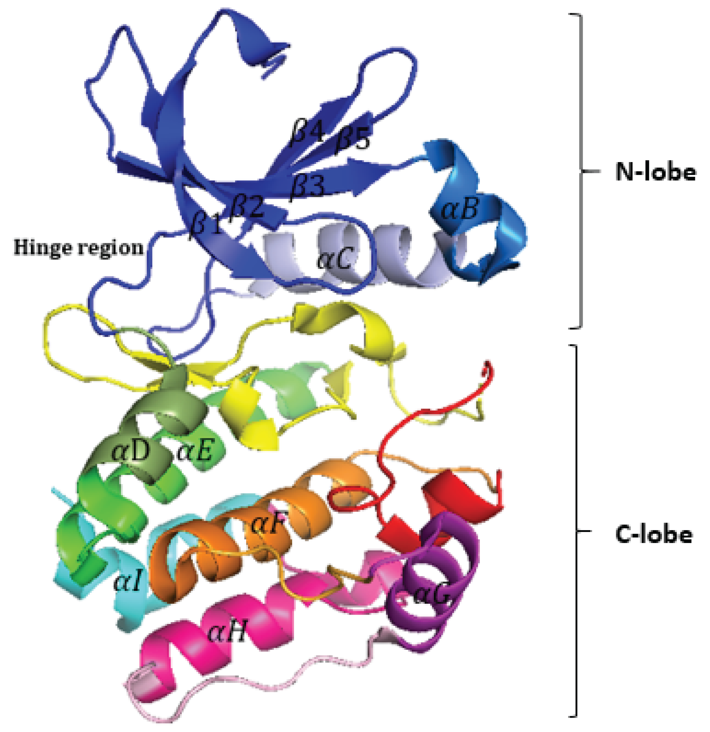
Figure 2. The Activation Segment of protein kinases (A) The structure of ABL1 (2G2H) showing the entire activation segment (orange). (B) Nomenclature of the activation segment. The activation segment runs from the conserved DFG to the conserved APE in the P+1 loop and includes β9 and the activation loop.

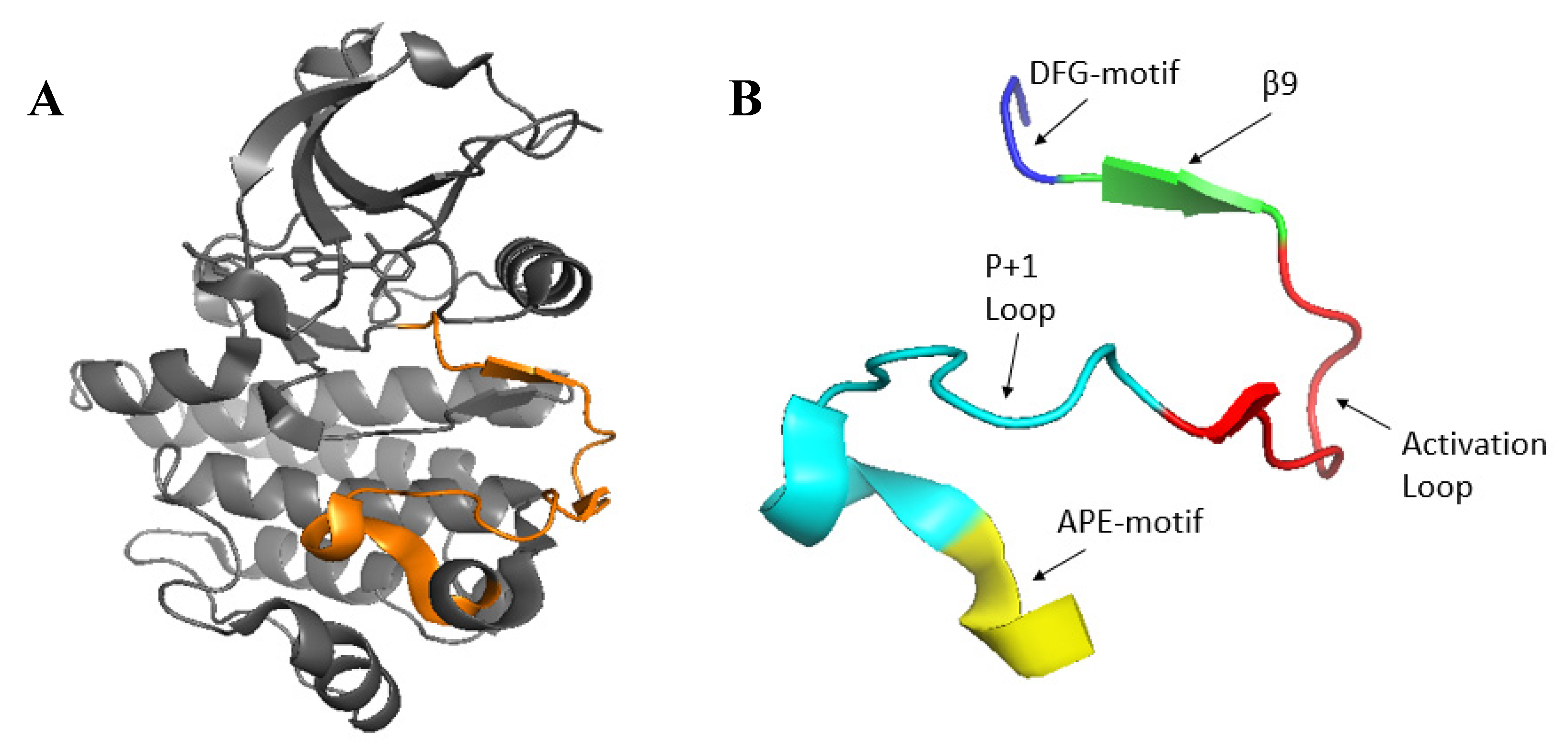
Figure 3. All active EPKs have a conserved internal architecture, but inactive structures can vary significantly. (A) Activation Segments of activated kinases typically have a highly conserved conformation. (B) Different kinases can be inactivated in different ways; therefore, an Activation Segment in its inactivated state can accept diverse conformations.

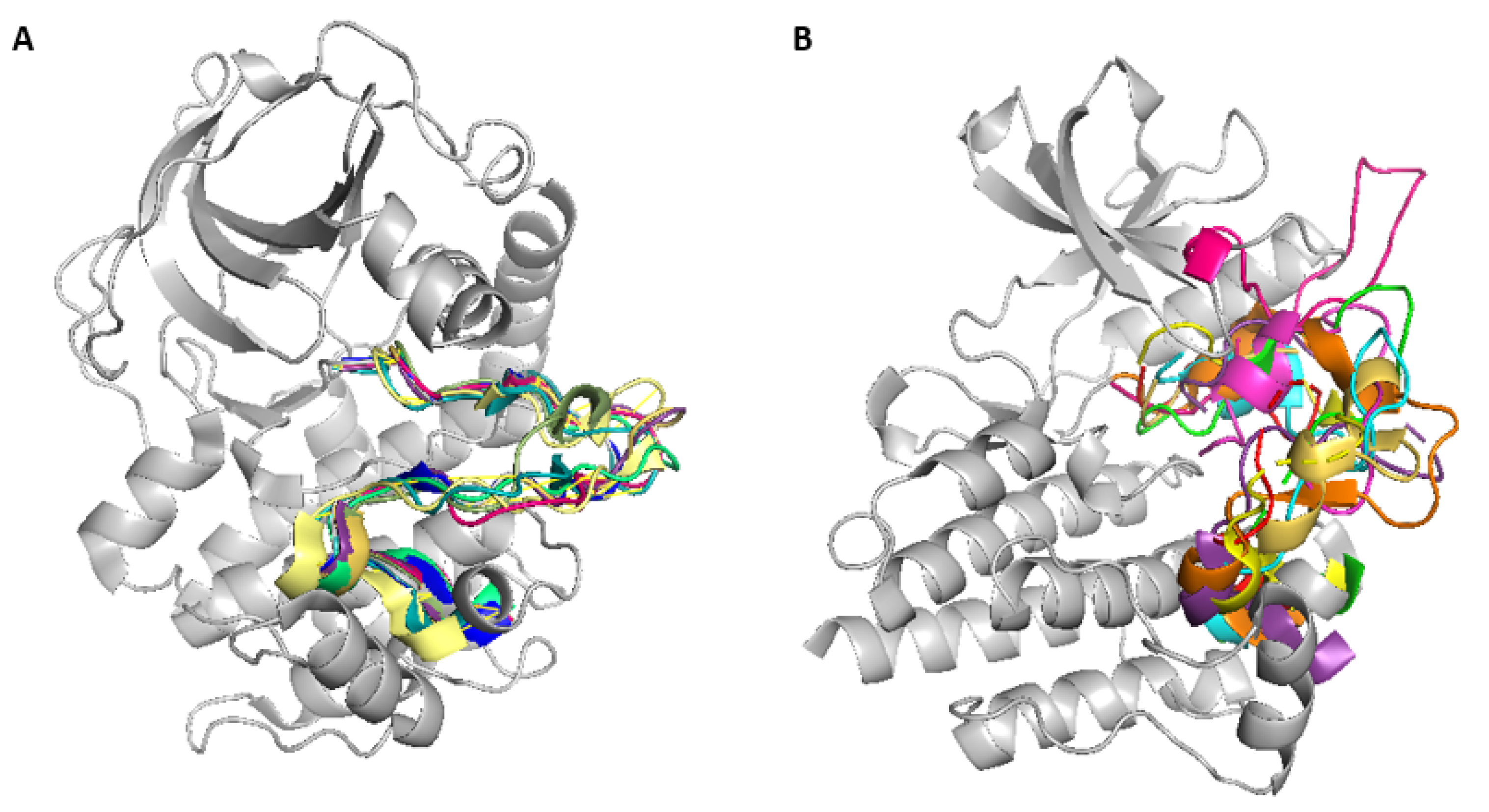
Figure 4. Similarity Analysis between Kinase Structures and Dataset Features. Similarity 1 compared kinase structure 4IAK (chain A) to all kinase features in the dataset, Similarity 2 compared 4DFZ (chain E), and Similarity 3 compared 4IAD (chain A). (A) The Manhattan distance metric. (B) The dot product similarity metric to assess structural similarity across kinase features.

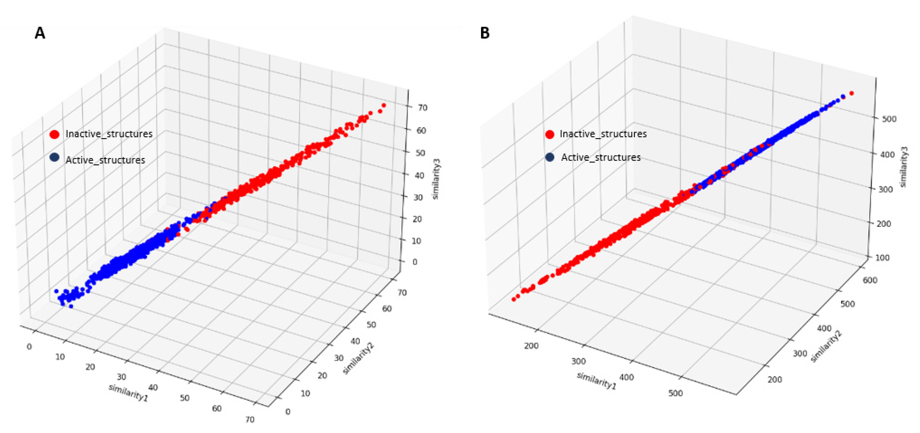
Figure 5. The assembly of the Regulatory spine in kinase structures (Active/Inactive). In the inactive BRAF (4KSP) (right) and active PAK4 (4L67) (middle), the R-spine is disrupted, whereas it remains intact in the active JAK2 (4GL9) (left).

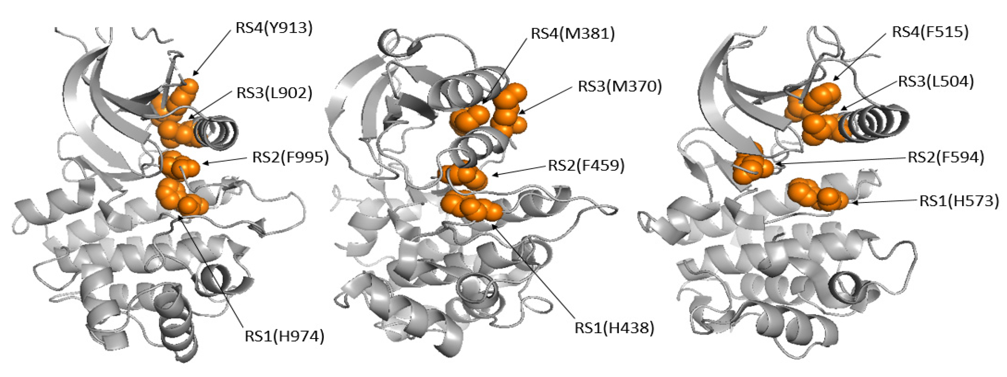
Table 1. Benchmark Model Performance - Training Set.

Model	Accuracy	Precision	Recall	F1 (Active)	F1 (Inactive)	ROC AUC	Confusion Matrix
SVM	0.9928	0.9840	1.0000	0.9919	0.9934	0.9996	[[983, 13], [0, 800]]
Logistic Regression	0.9911	0.9864	0.9938	0.9900	0.9919	0.9993	[[985, 11], [5, 795]]
Random Forest	1.0000	1.0000	1.0000	1.0000	1.0000	1.0000	[[996, 0], [0, 800]]
XGBoost	1.0000	1.0000	1.0000	1.0000	1.0000	1.0000	[[996, 0], [0, 800]]

Table 2. Benchmark Model Performance - Test Set.

Model	Accuracy	Precision		Recall	F1 (Active)	F1 (Inactive)	ROC AUC	Confusion Matrix
SVM	0.9911	0.9805	1.0000		0.9901	0.9919	1.0000	[[245, 4], [0, 201]]
Logistic Regression	0.9889	0.9804	0.9950		0.9877	0.9899	0.9985	[[245, 4], [1, 200]]
Random Forest	0.9956	0.9901	1.0000		0.9950	0.9960	0.9999	[[247, 2], [0, 201]]
XGBoost	0.9956	0.9950	0.9950		0.9950	0.9960	1.0000	[[248, 1], [1, 200]]

Table 3. Randomized Search Performance - Training Set.

Model	Accuracy	Precision	Recall	F1 (Active)	F1 (Inactive)	ROC AUC	Confusion Matrix
SVM	1.0000	1.0000	1.0000	1.0000	1.0000	1.0000	[[996, 0], [0, 800]]
Logistic Regression	0.9911	0.9864	0.9938	0.9900	0.9919	0.9993	[[985, 11], [5, 795]]
Random Forest	0.9967	0.9963	0.9963	0.9963	0.9970	0.9999	[[993, 3], [3, 797]]
XGBoost	0.9939	0.9901	0.9963	0.9931	0.9945	0.9998	[[988, 8], [3, 797]]

Table 4. Randomized Search Performance - Test Set.

Model	Accuracy	Precision	Recall	F1 (Active)	F1 (Inactive)	ROC AUC	Confusion Matrix
SVM	0.9889	0.9851	0.9901	0.9876	0.9899	0.9982	[[246, 3], [2, 199]]
Logistic Regression	0.9889	0.9804	0.9950	0.9877	0.9899	0.9984	[[245, 4], [1, 200]]
Random Forest	1.0000	1.0000	1.0000	1.0000	1.0000	1.0000	[[249, 0], [0, 201]]
XGBoost	0.9978	0.9950	1.0000	0.9975	0.9980	1.0000	[[248, 1], [0, 201]]

Table 5. Bayesian Results Performance - Training Set.

Model	Accuracy	Precision	Recall	F1 (Active)	F1 (Inactive)		ROC AUC	Confusion Matrix
SVM	0.9944	0.9901	0.9975	0.9938	0.9950	0.9993		[[988, 8], [2, 798]]
Logistic Regression	0.9911	0.9864	0.9938	0.9900	0.9919	0.9993		[[985, 11], [5, 795]]
Random Forest	0.9972	0.9975	0.9963	0.9969	0.9975	0.9999		[[994, 2], [3, 797]]
XGBoost	0.9955	0.9938	0.9963	0.9950	0.9960	0.9999		[[991, 5], [3, 797]]

Table 6. Bayesian Results Performance - Test Set.

Model	Accuracy	Precision	Recall	F1 (Active)	F1 (Inactive)	ROC AUC	Confusion Matrix
SVM	0.9933	0.9853	1.0000	0.9926	0.9939	1.0000	[[246, 3], [0, 201]]
Logistic Regression	0.9889	0.9804	0.9950	0.9877	0.9899	0.9985	[[245, 4], [1, 200]]
Random Forest	0.9956	0.9901	1.0000	0.9950	0.9960	1.0000	[[247, 2], [0, 201]]
XGBoost	0.9956	0.9901	1.0000	0.9950	0.9960	1.0000	[[247, 2], [0, 201]]

Table 7. Coordinate Descent Performance - Training Set.

Model	Accuracy	Precision	Recall	F1 (Active)	F1 (Inactive)	ROC AUC	Confusion Matrix
SVM	0.9972	0.9950	0.9988	0.9969	0.9975	0.9999	[[992, 4], [1, 799]]
Logistic Regression	0.9911	0.9864	0.9938	0.9900	0.9919	0.9993	[[985, 11], [5, 795]]
Random Forest	1.0000	1.0000	1.0000	1.0000	1.0000	1.0000	[[996, 0], [0, 800]]
XGBoost	0.9978	0.9963	0.9988	0.9975	0.9980	0.9999	[[993, 3], [1, 799]]

Table 8. Coordinate Descent Performance - Test Set.

Model	Accuracy	Precision	Recall	F1 (Active)	F1 (Inactive)	ROC AUC	Confusion Matrix
SVM	0.9956	0.9901	1.0000	0.9950	0.9960	0.9999	[[247, 2], [0, 201]]
Logistic Regression	0.9889	0.9804	0.9950	0.9877	0.9899	0.9985	[[245, 4], [1, 200]]
Random Forest	0.9978	0.9950	1.0000	0.9975	0.9980	1.0000	[[248, 1], [0, 201]]
XGBoost	0.9978	0.9963	1.0000	0.9975	0.9980	1.0000	[[248, 1], [0, 201]]

Table 9. Training Set Results (Probabilistic & Non-Parametric Models).

Model	Accuracy	Precision	Recall	F1 (Active)	F1 (Inactive)	ROC AUC	Confusion Matrix
GMM	0.9911	0.9937	0.9862	0.9900	0.9920	0.9997	[[789, 11], [5, 991]]
KDE	1.0000	1.0000	1.0000	1.0000	1.0000	1.0000	[[800, 0], [0, 996]]

Table 10. Training Set Results (Probabilistic & Non-Parametric Models).

Model	Accuracy	Precision	Recall	F1 (Active)	F1 (Inactive)	ROC AUC	Confusion Matrix
GMM	0.9844	0.9949	0.9701	0.9824	0.9861	0.9997	[[195, 6], [1, 248]]
KDE	0.9911	0.9805	1.0000	0.9901	0.9919	0.9994	[[201, 0], [4, 245]]

Table 11. Performance Comparison of Kinconform, KinActive, and Random Forest (Coordinate Descent) on All Datasets.

	Kinconform	KinActive	Random Forest (Coordinate Descent)(on all dataset)
Accuracy	0.9979	0.9991	0.9996
Precision	0.9975	0.9989	0.9990
Recall	0.9981	0.9994	1.0000
F1_score	0.9978	0.9992	0.9995
ROC_AUC	0.9979	0.9991	0.9996

Disclaimer/Publisher’s Note: The statements, opinions and data contained in all publications are solely those of the individual author(s) and contributor(s) and not of MDPI and/or the editor(s). MDPI and/or the editor(s) disclaim responsibility for any injury to people or property resulting from any ideas, methods, instructions or products referred to in the content.

© 2025 by the authors. Licensee MDPI, Basel, Switzerland. This article is an open access article distributed under the terms and conditions of the Creative Commons Attribution (CC BY) license (http://creativecommons.org/licenses/by/4.0/).

Copyright: This open access article is published under a Creative Commons CC BY 4.0 license, which permit the free download, distribution, and reuse, provided that the author and preprint are cited in any reuse.