
Submitted:
05 June 2025
Posted:
06 June 2025
You are already at the latest version
Abstract
The presence and control of bacteria in water distribution systems (WDS) is a global problem that warrants appropriate water disinfection that minimizes exposure, especially to pathogenic microorganisms. Chlorine is commonly used for drinking water disinfection, but the chlorine dose used should be balanced with the need to minimize the formation of byproducts. Therefore, modeling of residual chlorine is an interesting alternative to improve and control disinfection. In this study, the presence of bacteria in water samples from a WDS was monitored regularly and used together with added chlorine to model bacteria and free residual chlorine. This paper presents the application of two empirical models for predicting residual chlorine concentration and bacterial counts in a WDS. The first is a multiple linear regression model and the second is a nonlinear artificial neural network (ANN). The development of both models is based on representative data obtained from the Split-Dalmatia County continuous WDS in Croatia. The obtained results indicate that the developed model ANN can successfully describe the relationship between residual chlorine and bacterial count and can be used for estimation of residual chlorine and total bacterial count in WDS.
Keywords:
artificial neural network model
; disinfection
; drinking water
; mathematical modeling
; multiple linear regression model
; residual chlorine
1. Introduction
Water is essential for life, and water safety is important for both drinking water and water used for recreational or rehabilitative purposes. Appropriate research and improvements to public water systems are important to public health. The quality of water is regularly monitored at the source, after treatment and disinfection, in water reservoirs and then in distribution networks by measuring organoleptic, physical, chemical and microbiological properties. The supply of pure drinking water and the appropriate sanitation are of fundamental importance for the protection of the population against large-scale epidemics [1,2].
In Split-Dalmatia County, Croatia, geologically flysch and limestone are predominant. Where flysch and limestone meet, water springs gush, so Split-Dalmatia County is rich in surface water. The water from the catchment area of the Jadro River belongs to the typical karst waters, characterized by unique features such as specialized water circulation patterns, advanced karst erosion, distinct morphological and hydrographic characteristics, and a scarcity of surface water relative to a rich subterranean hydrographic network . The area of Split-Dalmatia County (SDC) is located on the central part of the eastern coast of the Adriatic Sea on an area of 4,501 km2 (about 8% of the surface of the Republic of Croatia) where about 450,000 inhabitants live, which is about 9% of the population of Croatia. The entire area of the cities of Split, Solin, Kaštela and Trogir is supplied with water from the karst source of the Jadro river [3,4,5,6,7,8,9,10]. The degree of connection of SDC residents to the water supply system is 80%. The water captured at the source of the Jadra is brought by gravity to the main pumping stations, and the necessary amounts of water are further distributed to the main reservoirs. The construction of the water supply system and the city network with associated water supply facilities was carried out in several stages, and was completed in 1956. The length of the network in the water supply system of the city of Split and surroundings is about 360 km and about 300,000 inhabitants are connected to it. The degree of connection of the population in the city of Split to the water supply system is 98%, while the rest use local water supply or from individual sources [11].
From the Jadro spring, water is drained on an average annual level of about 0.49 m3/s, which amounts to about m3 on average per year. During all these years, there have been no hydric epidemics, and this study is useful in order to make decisions about the exact amount of chlorine added in order to disinfect the water. Due to the specificity of the hydrogeological characteristics of karst aquifers, karst sources are particularly sensitive to pollution. During heavy rainfall or after long dry periods, pollution of karst springs is possible. Then there is a possibility of deterioration of drinking water quality, turbidity and short-term increased bacteriological contamination and will impact the amount of chlorine that needs to be added to the water.
However, it can be realistically expected that the air temperatures in the Mediterranean will rise in the future as a consequence of global warming. Drought occurrences will intensify during the summer and periods without rain, which could result in a renewed increase in water abstraction from the Jadro source. In general, it is recommended to maintain the lowest effective concentration of chlorine that ensures adequate disinfection without compromising the organoleptic properties of the water (taste and odor). This means that water supply operators should carefully balance the chlorine levels to ensure microbiological safety while avoiding excessive use. Overuse of chlorine can lead to unpleasant sensory changes and the formation of disinfection by-products at higher concentrations, which may have negative effects on human health.
The quality of surface water depends on the drained watershed area, location and sources of pollution, therefore water treatment is regulated to ensure its safety. In order to prevent diseases such as typhoid, dysentery, cholera and gastroenteritis, drinking water should be free of pathogenic microorganisms [1,12]. Disinfection is standardized and practiced treatment to remove pathogens from water. Chlorination is the prevalent technique employed in Croatia and worldwide to eliminate pathogenic microorganisms that could be found in drinking water. The quality of raw and chlorinated water is monitored by the water system managers. The presence and control of total bacterial count in water distribution systems (WDS) is important to minimize human exposure, especially to pathogenic microorganisms. The microbiological integrity of drinking water is a global problem that requires, among other things, disinfection of drinking water. Disinfection is performed to control pathogens, including primary and secondary bacterial pathogens (Escherichia coli, Klebsiella, Enterococcus faecalis, Campylobacter, Shigella, Helicobacter, Pseudomonas aeruginosa, Aeromonas hydrophila and others) and minimize the risk of exposure to human health [13].
1.1. Chlorination: Water Disinfection Process
Chlorination as a method of drinking water disinfection was first introduced in Belgium in 1902 [14]. Most WDSs in developed and developing countries use chlorine as a disinfectant [2,15,16]. Chlorination is the most common method to destroy the pathogenic organisms that may normally be present in Croatian drinking water [17]. The use of chlorine for drinking water disinfection served to prevent waterborne diseases and to ensure drinking water quality [18]. Chlorine readily combines with chemicals and organic compounds present in water. These components "consume" chlorine and account for the chlorine demand of the treatment system. It is crucial to add sufficient chlorine to the water in order to meet the chlorine demand and thus provide residual disinfection. The chlorine that does not combine with other components in the water is free residual chlorine, and the breakpoint is the point at which free chlorine is available for continuous disinfection. The contact in the process of chlorination refers to the period between the introduction of the chlorine and the end use of the water. Chlorine demand refers to the amount of chlorine that is consumed by chemicals and organic compounds present in water, as chlorine readily combines with these components during the treatment process. The required contact time can vary in relation to chlorine concentration, type of existing pathogens, pH and temperature of the water. In order to achieve adequate contact time, it is necessary to ensure complete mixing of chlorine and water, as well as to provide a holding tank for water retention. Chlorinator operation should be automatic, proportional to water flow and adjusted to the chlorine demand of the water. Disinfectant dosing is important to prevent microbial contamination, and the effectiveness of chlorine-based disinfectants depends on the concentration of total bacteria [19].
Authors in [20,21] reported that the use of chlorine for drinking water disinfection is to prevent waterborne diseases as they travel through the many kilometers of pipe. In drinking water, free residual chlorine will destroy most taste and odor and inhibit growth microorganisms inside water mains, thus correlated with the absence of disease-causing organisms and is a measure of the water’s potability. The problem of maintaining sufficient disinfectant residual throughout the distribution system cannot be solved by more often addition of more chlorine to the treatment plant [22]. Through disinfection process, chlorine reacts with natural organic matter present in the water and form products that have potentially harmful health effects. Through disinfection process, chlorine reacts with natural organic matter present in the water and form products that have potentially harmful health effects [23,24]. Therefore, water utilities must balance the need for disinfection with the need to minimize the formation of harmful by-products [25]. Delivery of drinking water without or with reduced residual chlorine can favor the growth of bacteria and create changes in microbial populations [26,27]. The Croatian National Standard [28] on drinking water quality is based on the Drinking Water Directive (EU) 2020/2184, which establishes the monitoring program and parameters (microbiological, chemical, and indicator) that need to be measured in order to protect people’s health from harmful effects.
Therefore, the common practice of applying solely chemical disinfection in Croatia, relying mainly on the content of residual chlorine as proof of disinfection effect, should be gradually changed following the positive experience of European countries. In the EU Drinking Water Directive 2020/2184, specific maximum allowed concentrations of free chlorine or total chlorine are not directly prescribed in the directive itself. Instead, the directive sets general guidelines and standards for water safety, including microbiological and chemical parameters, but does not specify precise chlorine concentrations in drinking water.
However, chlorination is commonly used as a disinfection method, and chlorine levels (free or total chlorine) can be regulated at the national level according to specific standards set by EU member states, taking into account EU guidelines and the recommendations of the World Health Organization (WHO). The WHO recommends that the level of free chlorine should not exceed 5 mg/L. This higher limit is set to prevent negative health effects that may arise from excessive chlorine concentrations while still ensuring effectiveness in pathogen elimination. According to the current Croatian regulation on drinking water quality, the maximum allowable concentration of free residual chlorine in water is 0.5 mg/L. The residual chlorine modeling in this study was presented as a valuable tool for monitoring water quality in the distribution network, allowing to control residual chlorine levels in this pandemic season [29] . Therefore, residual chlorine modeling appears to be an alternative to improve and control disinfection efficacy [30,31].
In this work, the occurrence of bacteria in WDS and the modeling of bacteria and free residual chlorine was studied. The total bacterial count was used as an indicator of disinfection performance. This paper presents the application of two empirical models for the prediction of residual chlorine concentration and bacterial count in WDS. The first is a multiple linear regression model (RM) and the second is a nonlinear artificial neural network model (ANN). The development of both models is based on representative data from drinking water systems in Croatia (Split-Dalmatia County). A model for analysis, assessment and prediction of drinking water quality was developed based on the results of the 6-year sanitary maintenance program conducted by the Teaching Institute for Public Health, Split-Dalmatia County in Croatia.
2. Materials and Methods
2.1. Water Sampling
In Split-Dalmatia County, Croatia a total of 5000 water samples were collected. The samples were collected from the water distribution system in Split-Dalmatia County, Croatia. Specifically:
- Raw water was collected from the Jadro River source, which is the main surface water source in the area.
- Chlorinated water samples were taken from bathroom taps in a hotel within the county, with the taps being disinfected by flame beforehand to ensure accurate results.
This location was chosen as it provides a representative analysis of water quality and disinfection efficiency within the distribution system. The sampling procedure adhered to ISO 19458:2006 [32] standards to ensure consistency and validity of the data for modeling purposes. To neutralize residual chlorine, water samples were collected in bottles containing sodium thiosulfate. This dechlorinating agent prevents chlorine from continuing to act on microorganisms during transport, ensuring accurate microbiological analysis. In order to neutralize the residual free chlorine, 0.5 mL of sodium thiosulfate ( Na2S2O35 H2O = 18 mg/mL) was added for 500 mL of bottle capacity for bacteriological analysis. Samples were stored at 4 °C and immediately taken to a laboratory for chemical and microbiological analysis.
2.2. Chemical and Microbiological Analyses
The process of water disinfection is carried out with gaseous chlorine, and it was carried out using a chlorinator. During the winter season (November-April) 0.35 mg/L of gaseous chlorine was initially added, and during the summer season (May-October) 0.5 mg/L. The residual free chlorine content was measured in the water supply network at the time of sample collection using a calibrated portable colorimeter according to the standard method (DPD method, HANNA Instruments 96734). Microbiological analyses were performed within six hours of sample collection. Microbiological parameters include determination of the total number of bacteria (aerobic mesophilic bacteria) on agar at a temperature of 37 °C, coliform bacteria, E. coli and enterococci. Cultivation and enumeration of the aerobic heterotrophic bacteria (HPC) was performed according to the standard ISO (EN ISO 6222:1999 [33]). An aliquot of a sample (1 mL) was placed in a sterile Petri dish and 18 mL of melted tempered Plate Count Agar medium (PCA; Oxoid Ltd, Basingstoke Hampshire, England) was added. The plates were gently swirled to mix the sample into the molten agar. After the agar was allowed to solidify at room temperature (no more than 15 minutes), the plates were inverted and incubated at 36±2 °C for 44±4 hours. C- EC agar (C- EC; Biolife, Milano, Italy) was used for the detection of total coliforms (TC) and E. coli (EC) analyses were performed according to the ISO standard (EN ISO 9308-1:2014/A1:2017 [34]). Isolation and enumeration of intestinal enterococci in water samples was performed according to the ISO standard on Slanetz and Bartley Agar (Slanetz and Bartley Agar, Liofilchem, Italy) (EN ISO 7899-2:2000 [35]).
The obtained results were expressed as the total number of bacteria (HPC, CFU/mL), Total Coliforms (TC, CFU/100 mL), intestinal enterococci count (ENT, CFU/100 mL), E. coli (EC, CFU/100 mL).
2.3. Application of Multiple Regression and the Artificial Neural Network Model
Multiple linear regression is used to create statistical models that describe the influence of one or more independent (predictor) variables - X on the dependent (response) variable - Y. The general form of multiple linear regression is given by the expression::
Where:
- Y - dependent variable (response),
- - independent variables (predictor),
- n - number of variables,
- - regression coefficients representing the relative predictive power of the model,
- c - constant that intersects the y-axis for the case .
The disadvantage of all regression techniques is the impossibility of determining the causal mechanism of the relationship between the dependent and independent variables, and the causal mechanism is determined by subsequent analysis.
Generally, multiple regression is separately applied to estimate the dependent variable Y (in this paper: - Cl and - HPC) depending on one or more independent variables X (in this paper: - added chlorine, - TC, - ENT, - EC).
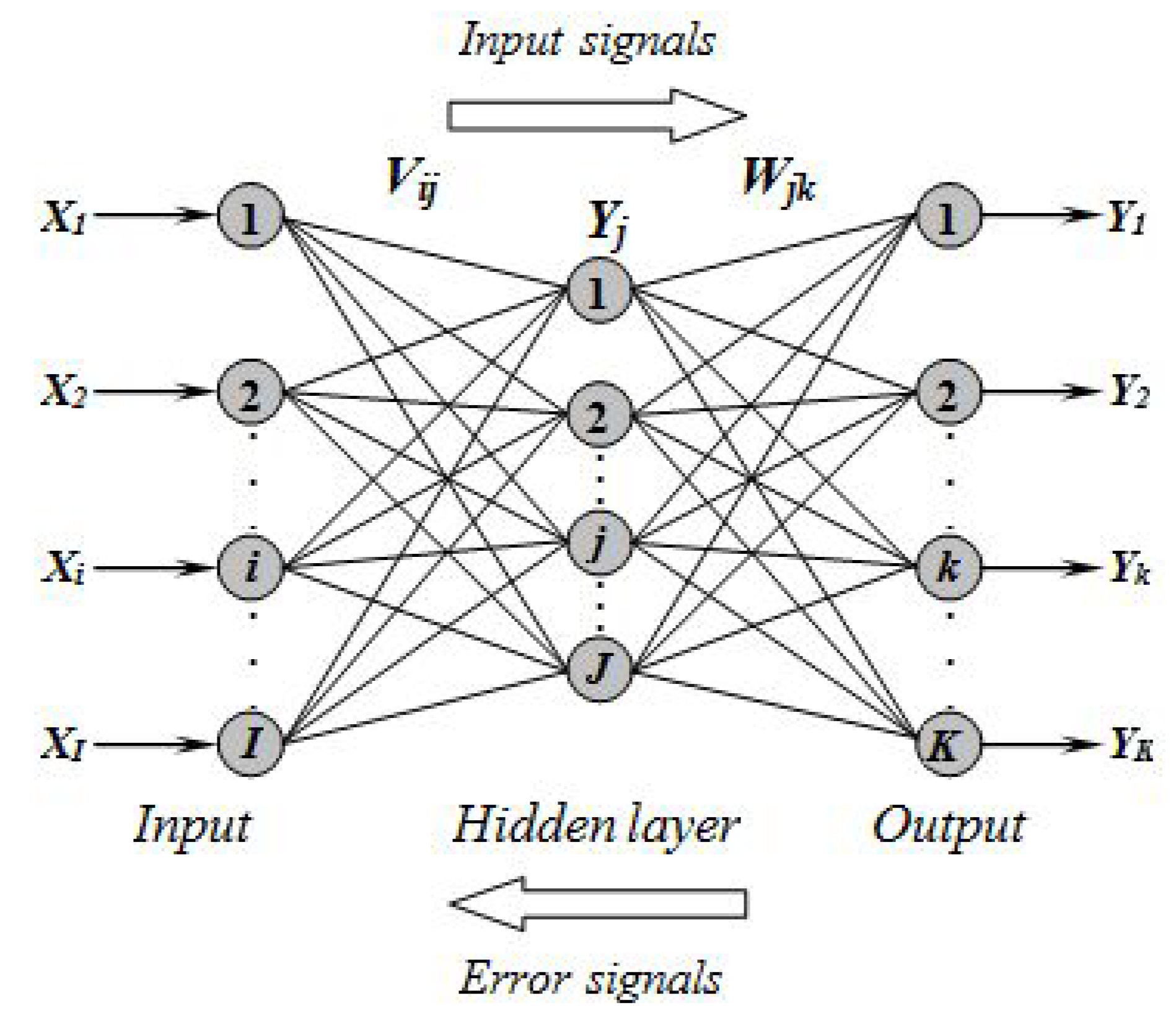
Artificial neural networks (ANN) are known for their ability to learn from historical data as opposed to rule-based models that use rules specified by the user. Multi-layer backpropagation neural network is most often used in practice. Backpropagation was created by generalizing the Widrow-Hoff learning rule to multiple-layer networks and nonlinear differentiable transfer functions [36]. Input vectors (independent variables) and corresponding transfer functions are used in the learning process of the neural network to approximate the value of the target variable (dependent variable). Multi-layer neural networks usually have several hidden layers with a different number of neurons and different transfer functions in each layer. Unlike the regression model, multiple layers neural networks with non-linear transfer functions enable the learning of linear and non-linear relationships between input (predictor) and output (response) vector variables. There are numerous variations of the basic neural network learning algorithm, and one of them is the so-called feedforward backpropagation training algorithm that minimizes the mean square error (MSE) between the actual (experimental) and the estimated value of the output variable by the neural network. The principle mode of operation of the feedforward backpropagation network learning algorithm is shown in Figure 1. The basic backpropagation training algorithm consists of the following steps and can be summarized as follows:
Figure 1.
The principle of the feedforward backpropagation training algorithm.
Step 1: Initialization of the values of weights and .
Step 2: Calculation of the value of each neuron in all layers:
Step 3: Compute the outputs:
where is: values of weights between the input layer and the hidden layer, - values of weights between the hidden layer and the output layer, - vector of input variables, i - number of neurons of the input layer, I - number of inputs of neuron j in the hidden layer, - output value of the hidden neurons, j - number of neurons of the hidden layer, J - number of inputs of neuron k in the output layer, - output signals and k - number of neurons of the output layer.
Sigmoidal transfer function is used in the hidden layers, and its equation is:
The input layer is made up by the following data: Added chlorine (X1), Total Coliforms - TC (X2), Intestinal enterococci- ENT (X3) and E. coli - EC (X4). The output layer is data of residual chlorine. The neural network model made up with 4 input neurons and 10-15-40 neurons in hidden layers and 2 output neuron is the result of experimental and practical experiences obtained during work [37,38,39]. The function of the sigmoidal type (tansig) and the function of the linear type (purelin) were applied as the transfer function of the first and second hidden layer respectively. As a training function, gradient descent with momentum and adaptive learning rate back-propagation function was applied. Training parameters of the ANN model are shown in Table 1. The software used in the research is Matlab.

Table 1.
ANN training parameters.
| Parameter | Value |
|---|---|
| Performance function - MSE | 0.0001 |
| Learning rate | 0.01 |
| Learning rate - increase | 0.5 |
| Learning rate - decrease | 1.05 |
| Maximum performance increase | 1.04 |
| Minimum performance gradient | 1e−10 |
| Momentum | 0.9 |
| Number of layers | 3 |
| Number of neurons | 10-15-40 |
| Transfer functions | tansig-tansig-purelin |
| Training function | Levenberg-Marquardt |
| Epochs to train | 1000 |
| Training ratio | 70% |
| Test ratio | 30% |
As the main measure for evaluating the quality of RM and ANN models, the statistical measure NRMSE (Normalized Root Mean Square Error) has been proposed 12. Lower NRMSE values indicate better model performance.
where is: N- Number of sample, dn-output experimental value (desired outputs), - output value of the model (actual outputs) and is the standard deviation.
3. Experimental Data
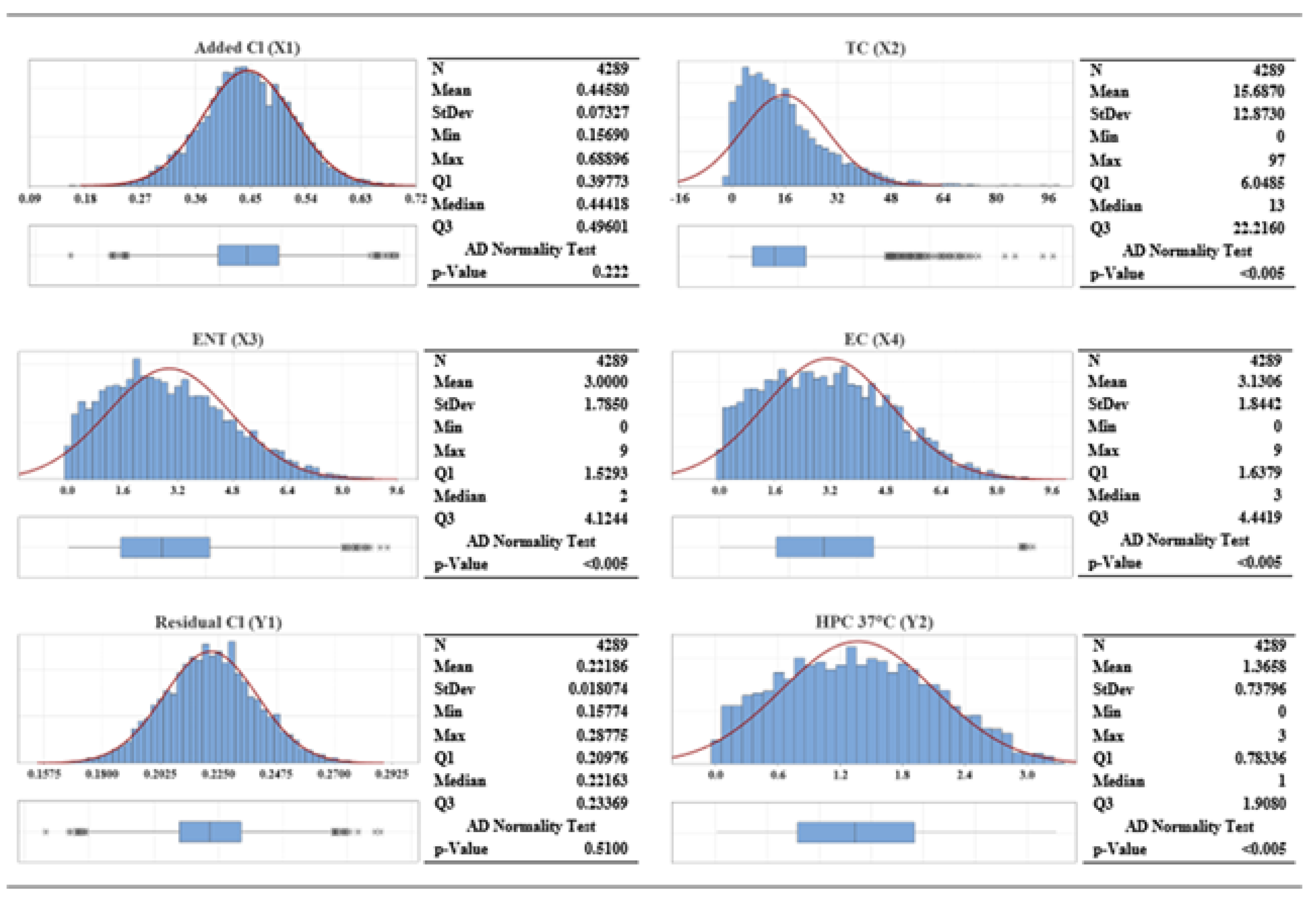
Jadro River water was analyzed and used to evaluate the ability of empirical modeling to predict residual chlorine and total bacterial count in the WDS. Total of 5000 samples were collected, and after exploratory data analysis and cleaning the set of missing data and outliers, 4289 samples remained for modeling. Figure 2 shows the data distribution and basic descriptive statistics of the microbiological analysis of the experimental data.
Figure 2.
Data distribution and descriptive statistics of experimental data.
4. Results and Discussion
In the following chapter, the results of the application of multiple linear regression modeling are shown. Later on, the artificial neural network (ANN) modeling is discussed, and a comparison of the RM/ANN models is made. The results of the multiple Stepwise linear regression modeling are presented in Table 2, Table 3, Table 4, and Table 5, respectively. Stepwise regression was used to discover the set of predictors () that best describe the response (). For this purpose, the following interactions of independent variables or predictors were created: , , , , , , , , , , , , , , . The criterion for accepting or omitting a predictor from the stepwise regression model is . For validation, the stepwise model was tested on 30% of the selected samples from the total set, while 70% of the data was used for model training. The same datasets (70/30) were used to train the ANN model.
Table 2.
The results of the Stepwise regression model for .
| Parameter | Coef | Stan. Error | T-Statistic | p-Value |
|---|---|---|---|---|
| CONSTANT | 0.31945 | 0.00128 | 250.20 | 0.000 |
| -0.20567 | 0.00243 | -84.68 | 0.000 | |
| -0.001610 | 0.000196 | -8.22 | 0.000 | |
| -0.000339 | 0.000098 | -3.46 | 0.001 | |
| 0.000056 | 0.000029 | 1.97 | 0.049 |
Table 3.
The results of the Analysis of Variance for Y1.
| Source | Df | Sum of Sq | Mean of Sq | F-Value | p-Value |
|---|---|---|---|---|---|
| Model | 4 | 0.693818 | 0.173454 | 1855.86 | 0.000 |
| X1 | 1 | 0.670142 | 0.670142 | 7170.13 | 0.000 |
| X3 | 1 | 0.006312 | 0.006312 | 67.54 | 0.000 |
| X4 | 1 | 0.001116 | 0.001116 | 11.94 | 0.001 |
| X3*X4 | 1 | 0.000362 | 0.000362 | 3.87 | 0.049 |
| Error | 2997 | 0.280109 | 0.000093 | ||
| Total | 3001 | 0.973926 | |||
| Standard Error of Est. = 0.0096676 | |||||
Table 4.
The results of the Stepwise regression model for .
| Parameter | Coef | Stan. Error | T-Statistic | p-Value |
|---|---|---|---|---|
| CONSTANT | 1.8335 | 0.044 | 41.26 | 0.000 |
| -0.1853 | 0.0127 | -14.54 | 0.000 | |
| 0.02208 | 0.00638 | 3.46 | 0.001 | |
| -0.00367 | 0.00186 | -1.97 | 0.048 |
Table 5.
The results of the Analysis of Variance for Y2.
| Source | Df | Sum of Sq | Mean of Sq | F-Value | p-Value |
|---|---|---|---|---|---|
| Model | 3 | 420.56 | 140.185 | 354.38 | 0.000 |
| X3 | 1 | 83.67 | 83.665 | 211.50 | 0.000 |
| X4 | 1 | 4.73 | 4.734 | 11.97 | 0.001 |
| X3*X4 | 1 | 1.54 | 1.542 | 3.90 | 0.048 |
| Error | 2998 | 1185.93 | 0.396 | ||
| Total | 3001 | 1606.49 | |||
| Standard Error of Est. = 0.628948 | |||||
As can be seen from the regression equations (15) and (16), the independent variable is omitted because it has no effect on the change of the dependent variable (residual chlorine concentration) and (total number of aerobic heterotrophic bacteria). From Table 2, Table 3, Table 4, and Table 5, it is evident that for both models and , constants and predictor variables significantly affect the value of the model’s response because p-values are .
The variance analysis shows that the regression -model explains of the variability of the response data around its mean, and the contribution of predictor variables , , , and is (Table 2 and Table 3). The regression -model explains of the variability of the response data around its mean, and the contribution of predictor variables , , and is (Table 4 and Table 5).
The prediction ability of Residual Cl and Total number of bacteria regression models (RM) is satisfactory for response but unsatisfactory for response . To improve it, a feedforward ANN will be applied. RM and ANN models will be compared using performance indices: R, , SSE, MSE, RMSE, and NRMSE.
It is common practice to control chlorine dosing using raw water quality data and chlorine residual data at strategic points in the WDS. Modeling from ANN is used in many research studies to model and predict residual chlorine in the WDS. The variables used in these studies are typically chlorine concentration, flow, temperature, and pH [44,45,46]. Therefore, the presence of bacteria in the water is an important parameter to be considered and could improve the determination of the correct dose of added chlorine. Added Cl (), Intestinal enterococci (), and () will be used as independent variables to describe the relationship between residual chlorine () and total number of aerobic heterotrophic bacteria () in separate ANN models (Figure 3 and Figure 4). To compare the results for both ANN models, the same data set was used for training and validation as with the stepwise regression.
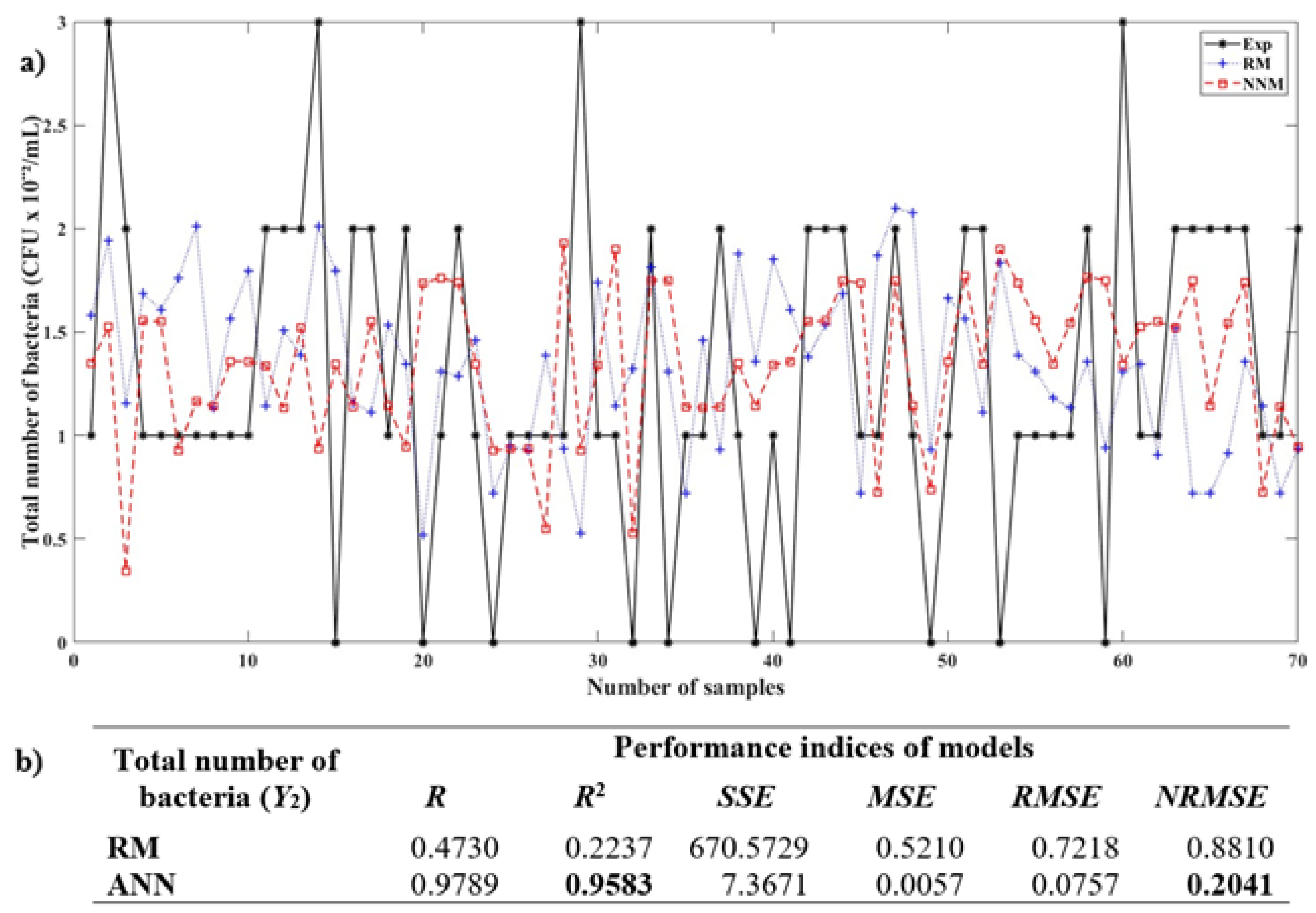
The performance indices indicate that the RM model, as fitted, explains 68.48% of the variability in the residual chlorine () and 22.37% of the total number of bacteria (). Analysis of variance also showed that all independent variables , , , and their interactions in both models significantly influence () the response variables and . Equations 15 and 16 of RM models are simplified by omitting variable while performing stepwise regression. In contrast to the RM model, the -statistic of the ANN-model explains 96.68% and 95.83% of the variability in and , respectively. The performance indices ANN-NRMSE for the case of residual chlorine is 0.1821, significantly lower than the indices RM-NRMSE (0.5621) as shown in Figure 3. The ANN-NRMSE performance indices for the total bacteria count is 0.2041 and is also significantly lower than the RM-NRMSE indices (0.8810) as shown in Figure 4. The plots in Figure 3 and Figure 4 show that the ANN model approximates the experimental test data better than the RM model. Similar observations after comparing the regression and artificial neural network model were previously reported in the study of chlorine residual prediction in the water distribution system [44]. With these considerations, the use of the neural network as a nonlinear model for estimating the residual chlorine and the total number of bacteria in the water distribution system is justified.
Figure 3.
Comparison of RM/ANN models to estimate residual chlorine () on the test data set (1287 samples). Fitting results of the 70 randomly selected samples (a) and (b) Performance indices of the models.
Figure 3.
Comparison of RM/ANN models to estimate residual chlorine () on the test data set (1287 samples). Fitting results of the 70 randomly selected samples (a) and (b) Performance indices of the models.
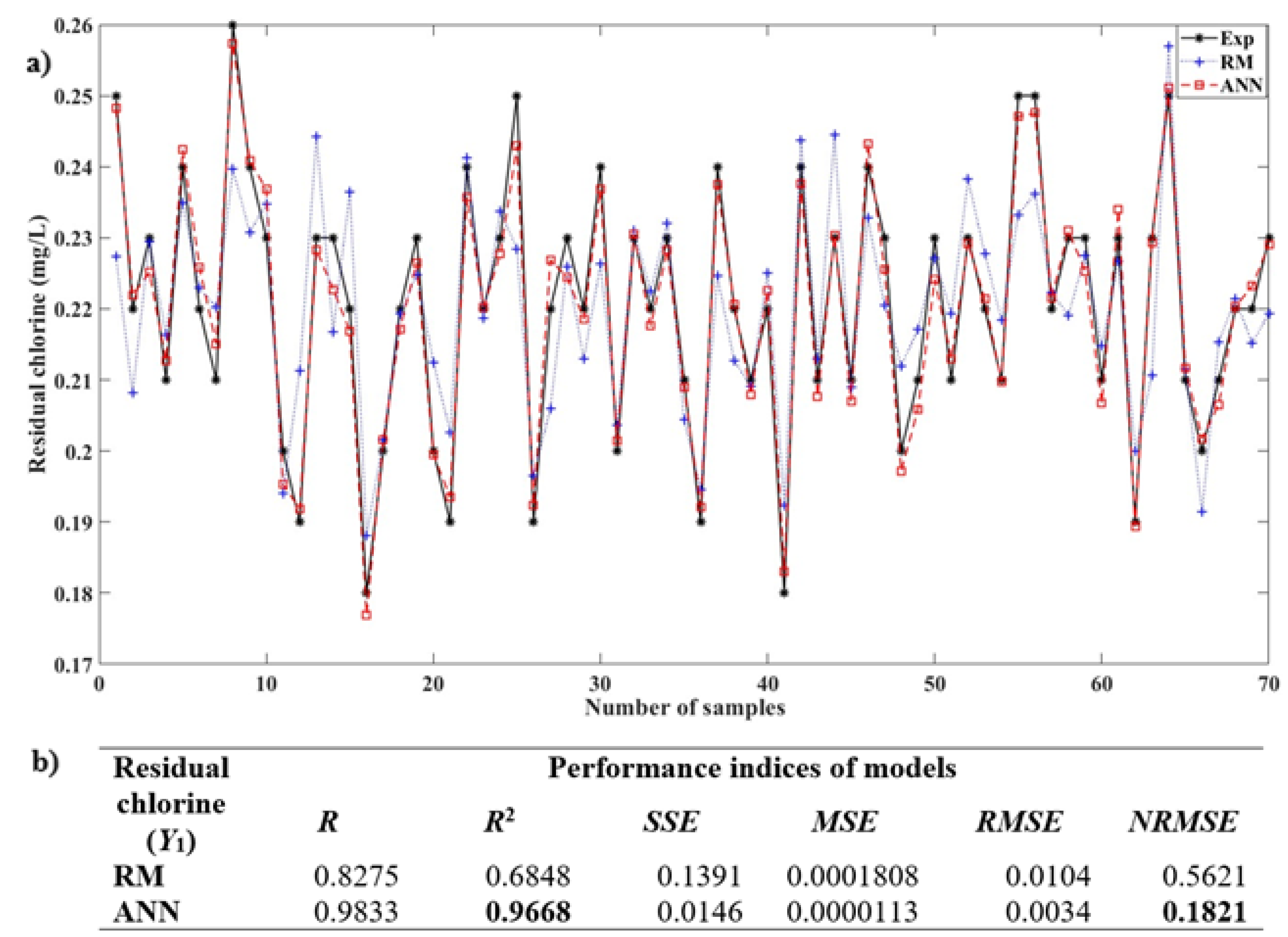
Figure 4.
Comparison of RM/ANN models to estimate the total number of bacteria () on the test data set (1287 samples). Fitting results of the 70 randomly selected samples (a) and (b) Performance indices of the models.
Figure 4.
Comparison of RM/ANN models to estimate the total number of bacteria () on the test data set (1287 samples). Fitting results of the 70 randomly selected samples (a) and (b) Performance indices of the models.
5. Conclusions
In this work, the occurrence of bacteria in raw and treated water samples was monitored within the WDS during the 6-year sanitary maintenance program in Split-Dalmatia County, Croatia, and the obtained results were used for modeling free residual chlorine and total number of bacteria. For this purpose, two empirical models were applied to obtain reliable predictions of residual chlorine concentration and number of bacteria in the WDS. The development of the RM model and an ANN model is based on the presence of added Cl, intestinal enterococci, E. coli is used as an independent variable to describe the relation ship between residual chlorine and the total number of bacteria within the WDS. The use of microbiological analysis values as an independent input variables and the comparison of the results obtained with the two applied models, showed that the application of the developed artificial neural network models provided a reliable estimation of the residual chlorine and the total number of aerobic heterotrophic bacteria from water supply systems supplied from karst sources. According to the multiple regression results (Table 2 and Table 3), the significant independent variables with the most impact on (Residual Chlorine) include:
- (added chlorine): This has the largest impact, with a high regression coefficient, indicating a direct relationship between the amount of added chlorine and the residual chlorine concentration.
- (enterococci): This has a smaller but statistically significant negative impact.
- The interaction term (enterococci ×): This shows the smallest but significant positive impact.
For (total number of aerobic heterotrophic bacteria), according to Table 4 and Table 5, the significant variables include:
- (enterococci): This has the largest negative impact on the total bacterial count.
- (E. coli): This has a positive impact, but smaller compared to .
- The interaction term : This has a significant negative impact.
RM is limited to linear relationships and simpler interaction effects, while more complex nonlinear relationships often remain uncaptured.
In contrast to the RM model, ANN automatically integrates interaction effects and nonlinearities through its hidden layers, enabling dynamic learning of these relationships during the training process. The superior performance of the ANN model is evident from the NRMSE indicator, which is for predicting (residual chlorine), and for predicting (total number of aerobic heterotrophic bacteria). In both cases, the ANN model’s NRMSE is significantly lower compared to the RM model.
Therefore, for future research, a combination of models is suggested: ANN for prediction and RM for interpretation, to leverage the advantages of both approaches.
Abbreviations
The following abbreviations are used in this manuscript:
| ak | Actual outputs of Eq. |
| Actual outputs (estimation) of Eqs. | |
| ANN | Artificial neural network |
| b1, b2, …, bn | The regression coefficients of Eq. |
| c | Constant of Eq. |
| Df | Degrees of freedom |
| dk | Desired outputs (experimental values) of Eq. |
| dn | Desired outputs (target) of Eqs. |
| E | System error. |
| Exp | Experimental. |
| I | Number of inputs of neuron j in the hidden layer of Eqs. |
| i | Number of neurons of the input layer of Eqs. |
| J | Number of inputs of neuron k in the output layer of Eqs. |
| j | Number of neurons of the hidden layer of Eqs. |
| K | Total number of patterns of Eq. |
| k | Number of neurons of the output layer of Eq. |
| lr | Learning rate of Eqs. |
| MCL | Maximum contaminant level |
| MR | Multiple regression |
| MSE | Mean square error |
| n | Current iteration step of Eqs. |
| NRMSE | Normalized Root Mean Square Error |
| N | Total number of patterns of Eqs. |
| R | Correlation coefficient |
| R2 | The square of correlation coefficients |
| RMSE | Root Mean Square Error |
| SSE | Sum of squared errors |
| T-Statistic | Student t distribution |
| V | Weight between the input layer and the hidden layer of Eq. |
| WDS | Water distribution systems |
| Weight between the hidden layer and the output layer of Eq. | |
| X | Independent variable |
| Added chlorine, mg/L | |
| - TC | Total coliforms, CFU×10−2/mL |
| - ENT | Intestinal enterococci, CFU×10−2/mL |
| X4 - EC | Escherichia coli, CFU×10−2/mL |
| Xi | Input signals |
| Y | Dependent variable of Eq. |
| Y1 | Residual chlorine, mg L−1 |
| Y2 - HPC | Total number of aerobic heterotrophic bacteria, CFU/mL |
| Output of the hidden neurons of Eqs. | |
| Y | Output signals |
| Momentum of Eqs. | |
| Learning errors of Eqs. | |
| Standard deviation of Eqs. |
References
- Chowdhury, S. Heterotrophic bacteria in drinking water distribution system: a review. Environ Monit Assess 2012, 184, 6087–6137. [Google Scholar] [CrossRef] [PubMed]
- NHMRC. Australian Drinking Water Guidelines Paper 6 National Water Quality Management Strategy. Technical report, Canberra, 2011.
- Štambuk Giljanović, N. Water quality evaluation by index in Dalmatia. Water Res 1999, 33, 3423–3440. [Google Scholar] [CrossRef]
- Fiorillo, F.; Pagnozzi, M.; Addesso, R.; Cafaro, S.; D’Angeli, I.M.; Esposito, L.; Leone, G.; Liso, I.S.; Parise, M. Uncertainties in understanding groundwater flow and spring functioning in karst. In Threats to Springs in a Changing World: Science and Policies for Protection; Currell, M.J., Katz, B.G., Eds.; American Geophysical Union: Washington D.C, 2022; pp. 131–143. [Google Scholar]
- Jukić, D.; Denić-Jukić, V. Investigating relationships between rainfall and karst-spring discharge by higher-order partial correlation functions. Journal of Hydrology 2015, 530, 24–36. [Google Scholar] [CrossRef]
- Jukić, D.; Denić-Jukić, V.; Kadić, A. Temporal and spatial characterization of sediment transport through a karst aquifer by means of time series analysis. Journal of Hydrology 2022, 609, 127753. [Google Scholar] [CrossRef]
- Margeta, J. Water abstraction management under climate change: Jadro spring Croatia. Groundwater for Sustainable Development 2022, 16, 100717. [Google Scholar] [CrossRef]
- Margeta, J.; Fistanić, I. Water quality modelling of Jadro Spring. Water Sciences and Technology 2004, 50, 59–66. [Google Scholar] [CrossRef]
- Rađa, B.; Puljas, S. Macroinvertebrate diversity in the karst Jadro river (Croatia). Archives of Biological Sciences 2008, 60, 437–448. [Google Scholar] [CrossRef]
- Štambuk Giljanović, N. Vode Dalmacije; Nastavni Zavod za javno zdravstvo Splitsko-dalmatinske županije: Split, 2006. [Google Scholar]
- Bonacci, O.; Roje-Bonacci, T. Analiza oduzimanja vode iz izvora Jadra u razdoblju 2010. - 2021. Hrvatske vode 2023, 31, 27–36. [Google Scholar]
- Cabral, J. Water Microbiology. Bacterial Pathogens and Water. Int J Environ Res Public Health 2010, 7, 3657–3703. [Google Scholar] [CrossRef]
- Rutala, W.; Weber, D. Guideline for Disinfection and Sterilization in Healthcare Facilities 2008.
- IARC. , Ed. Chlorinated drinking-water; chlorination by-products; some other halogenated compounds; cobalt and cobalt compounds; Number 52, IARC: Lyon, 1991. [Google Scholar]
- Panguluri, S.; Grayman, W.; Clark, R. Water Distribution System Analysis: Field Studies, Modeling, and Management 2005.
- EC. Council Directive 98/83/EC on the Quality of Water Intended for Human Consumption, L 330/32 ed. Official journal of the European Communities Council.
- Mansor, N.A.; Tay, K.S. Potential toxic effects of chlorination and UV/chlorination in the treatment of hydrochlorothiazide in the water. Sci Total Environ 2020, 20, 136745–136745. [Google Scholar] [CrossRef]
- Kim, H.; Kim, S.; Koo, J. Prediction of Chlorine Concentration in Various Hydraulic Conditions for a Pilot Scale Water Distribution System. Procedia Eng 2014, 70, 934–942. [Google Scholar] [CrossRef]
- Flemming, H.C.; Wingender, J.; Szewzyk, U. (Eds.) Biofilm highlights; Springer series on biofilms, Springer: Heidelberg ; New York, 2011. OCLC: ocn729346877.
- Moritz, M.M.; Flemming, H.C.; Wingender, J. Integration of Pseudomonas aeruginosa and Legionella pneumophila in drinking water biofilms grown on domestic plumbing materials. Int J Hyg Environ Health 2010, 213, 190–197. [Google Scholar] [CrossRef] [PubMed]
- Wimpenny, J.; Manz, W.; Szewzyk, U. Heterogeneity in biofilms. FEMS Microbiol Rev 2000, 24, 661–671. [Google Scholar] [CrossRef] [PubMed]
- Legay, C.; Rodriguez, M.J.; Sérodes, J.B.; Levallois, P. The assessment of population exposure to chlorination by-products: a study on the influence of the water distribution system. Environ Health 2010, 9, 59–73. [Google Scholar] [CrossRef]
- Legay, C.; Rodriguez, M.J.; Sadiq, R.; Sérodes, J.B.; Levallois, P.; Proulx, F. Spatial variations of human health risk associated with exposure to chlorination by-products occurring in drinking water. J Environ Manage 2011, 92, 892–901. [Google Scholar] [CrossRef]
- Zhang, X.; Yang, H.; Wang, X.; Fu, J.; Xie, Y.F. Formation of disinfection by-products: effect of temperature and kinetic modeling. Chemosphere 2013, 90, 634–639. [Google Scholar] [CrossRef]
- Speight, V.; Pirnie, M. Distribution Systems: The Next Frontier. The Bridge, National Academy of Engineering 2008, 38, 31–37. [Google Scholar]
- Bertelli, C.; Courtois, S.; Rosikiewicz, M.; Piriou, P.; Aeby, S.; Robert, S.; Loret, J.F.; Greub, G. Reduced Chlorine in Drinking Water Distribution Systems Impacts Bacterial Biodiversity in Biofilms. Frontiers in Microbiology 2018, 9, 2520. [Google Scholar] [CrossRef]
- Adefisoye, M.A.; Olaniran, A.O. Does Chlorination Promote Antimicrobial Resistance in Waterborne Pathogens? Mechanistic Insight into Co-Resistance and Its Implication for Public Health. Antibiotics 2022, 11. [Google Scholar] [CrossRef]
- Ordinances on compliance parameters, methods of analysis and monitoring of water intended for human consumption. Official Gazette of the Republic of Croatia 64/2023, 2023.
- García-Ávila, F.; Avilés-Añazco, A.; Ordoñez-Jara, J.; Guanuchi-Quezada, C.; Flores del Pino, L.; Ramos-Fernández, L. Modeling of residual chlorine in a drinking water network in times of pandemic of the SARS-CoV-2 (COVID-19). Sustainable Environment Research 2021, 31, 12. [Google Scholar] [CrossRef]
- Fisher, I.; Kastl, G.; Sathasivan, A. A suitable model of combined effects of temperature and initial condition on chlorine bulk decay in water distribution systems. Water Res 2012, 46, 3293–3303. [Google Scholar] [CrossRef] [PubMed]
- Xu, J.; Huang, C.; Shi, X.; Dong, S.; Yuan, B.; Nguyen, T.H. Role of drinking water biofilms on residual chlorine decay and trihalomethane formation: An experimental and modeling study. Sci Total Environ 2018, 642, 516–525. [Google Scholar] [CrossRef] [PubMed]
- International Organization for Standardization (ISO), Geneva, Switzerland. Water Quality - Sampling for Microbiological Analysis, 2006.
- International Organization for Standardization (ISO), Geneva, Switzerland. Water quality - Enumeration of culturable micro-organisms - Colony count by inoculation in a nutrient agar culture medium, 1999.
- International Organization for Standardization (ISO), Geneva, Switzerland. Water quality – Enumeration of Escherichia coli and coliform bacteria – Part 1: Membrane filtration method for waters with low bacterial background flora, 2017. ISO 9308-1:2014/Amd 1:2016; EN ISO 9308-1:2014/A1:2017.
- International Organization for Standardization (ISO), Geneva, Switzerland. Water quality - Detection and enumeration of intestinal enterococci - Part 2: Membrane filtration method, 2000.
- Glavaš, Z.; Lisjak, D.; Unkić, F. The Application of Artificial Neural Network in the Prediction of the As-cast Impact Toughness of Spheroidal Graphite Cast Iron. Kovové Materiály 2007, 45, 41–49. [Google Scholar]
- Cosic, P.; Lisjak, D.; Antolic, D. Regression analysis and neural networks as methods for production time estimation. Technical Gazette 2011, 18, 479–484. [Google Scholar]
- Lisjak, D.; Maric, G.; Štefanić, N. Studying the possibility of neural network application in the diagnostics of a small four-stroke petrol engine by wear particle content. Technical Gazette 2012, 19, 857–862. [Google Scholar]
- Živko Babić, J.; Lisjak, D.; Ćurković, L.; Jakovac, M. Estimation of chemical resistance of dental ceramics by neural network. Dent Mater 2008, 24, 18–27. [Google Scholar] [CrossRef]
- Löschel, A. Technological change in economic models of environmental policy. Ecol Econ 2002, 43, 105–126. [Google Scholar] [CrossRef]
- Mata, J. Interpretation of concrete dam behaviour with artificial neural network and multiple linear regression models. Eng Struct 2011, 33, 903–910. [Google Scholar] [CrossRef]
- Petrović, M.S.; Šoštarić, T.D.; Pezo, L.L. Usefulness of ANN-based model for copper removal from aqueous solutions using agro industrial waste materials. Chem Ind Chem Eng Q 2015, 21, 249–259. [Google Scholar] [CrossRef]
- Liu, X.; Kang, S.; Li, F. Simulation of artificial neural network model for trunk stem flowof Pyrus pyrifolia and its comparison with multiple-linear regression. Agric Water Manage 2009, 96, 939–945. [Google Scholar] [CrossRef]
- Bowden, G.J.; Nixon, J.B.; Dandy, G.C.; Maier, H.R.; Holmes, M. Forecasting chlorine residuals in a water distribution system using a general regression neural network. Math Comput Model 2006, 44, 469–484. [Google Scholar] [CrossRef]
- Rodriguez, M.J.; Sérodes, J.B. Assessing empirical linear and non-linear modelling of residual chlorine in urban drinking water systems. Environ Model Softw 1999, 14, 93–102. [Google Scholar] [CrossRef]
- Singh, K.P.; Gupta, S. Artificial intelligence based modeling for predicting the disinfection by-products in water. Chemom Intell Lab Syst 2012, 114, 122–131. [Google Scholar] [CrossRef]
Disclaimer/Publisher’s Note: The statements, opinions and data contained in all publications are solely those of the individual author(s) and contributor(s) and not of MDPI and/or the editor(s). MDPI and/or the editor(s) disclaim responsibility for any injury to people or property resulting from any ideas, methods, instructions or products referred to in the content. |
© 2025 by the authors. Licensee MDPI, Basel, Switzerland. This article is an open access article distributed under the terms and conditions of the Creative Commons Attribution (CC BY) license (https://creativecommons.org/licenses/by/4.0/).
Copyright: This open access article is published under a Creative Commons CC BY 4.0 license, which permit the free download, distribution, and reuse, provided that the author and preprint are cited in any reuse.


