
Submitted:
04 June 2025
Posted:
06 June 2025
You are already at the latest version
Abstract
Infinities and singularities pose a problem in physics and results in the inability to interpret equations in some extreme conditions. Aim of this paper is to create a semi-structured complex framework that treats infinities and singularities as evanescent waves that can be manipulated algebraically to produce logical, consistent and experimentally verifiable results. The framework utilizes semi-structured complex numbers (an algebra created to enable division by zero), state space modelling and a novel characteristic wave function as components to create novel evanescent functions that mathematically describe and interpret infinities and singularities in science equations. The utility of the framework is demonstrated in eight use cases drawn from classical mechanics, quantum mechanics and quantum field theory. The framework is robust enough to be used in any science where interpretations are needed in equations where infinities and singularities may arise during calculations.
Keywords:
infinities and singularities
; semi‐structured complex numbers
; evanescent waves
; quantum mechanics
; quantum field theory
1.0. Introduction
Infinities and singularities often arise in equations and are seen as a problem in physics. They prevent logical, consistent predictions from being made particularly in extreme conditions. Usually these infinities and singularities arise because of division by zero, integrating across infinities or in logarithmic functions. In physics where it is physically impossible to conduct experiments for example at the center of a black hole or determining phenomenon at the subatomic scale predictions need to be made from equations. However when these equation sealed infinities or singularities this means that the equations have reached their predictive limit. Physicists have attempted to solve this problem using ad hoc methods. For example in quantum field theory, when trying to calculate the transitional amplitude from a group of propagators regularization and renormalization techniques are used to eliminate infinities that arise. However these methods cannot be applied universally across all physics. There is no universally acceptable methods for dealing with infinities and singularities that arise in physics.
This paper aims to provide a robust universal method for dealing with infinities and singularities that arise in physics by creating a novel framework called the Semi-structured Complex Framework. Creating such a framework would enable predictions to be made particularly in extreme situations where experimental data is either unavailable or very difficult to obtain. With such a framework questions like “what's the curvature of space-time at the center of a non-rotating black hole?” and “what's the period of a simple pendulum if there is 0 gravity” can be answered.
To construct the semi-structured complex framework there needs to be an understanding of the following concepts: semi-structured complex numbers, state space modeling, propagation constant and evanescent waves.
1.1. Semi-Structured Complex Numbers
Semi-structured complex numbers are numbers that were created specifically to enable division by zero in regular algebraic equations. Semi-structured complex number set can be defined as follows:
A semi-structured complex number is a three-dimensional number of the general formthat is, a linear combination of real (), imaginary () and unstructured () units whose coefficientsare realnumbers.
The number is called semi-structured complex because it contains a structured complex part and an unstructured part . Integer powers of yield the following cyclic results:
Given the definition of semi-structured complex numbers, it can clearly be seen that infinity (represented by division by zero) is encoded within the number and can be dealt with algebraically. Other important characteristics of semi-structured complex numbers is given in Table 3 in Appendix 1.
Semi-structured complex numbers can be seen as vectors in a 3-dimensional Euclidean semi-structured complex space. This representation enables vector operations (such as addition, dot product, inner product) to be performed on semi-structured complex numbers.
1.2. State Spaces
In physics, a state space represents all possible states of a system, often visualized as a geometric space where each point corresponds to a unique state, and the system's evolution is described by how these points move over time. A classic example of where state space is used to represent a physical system is in particle spin. A particle spin is an intrinsic angular momentum. Intrinsic Angular Momentum is a form of angular momentum, but unlike the orbital angular momentum of a rotating object, it's an intrinsic property, meaning it's a fundamental characteristic of the particle, not something it gains from moving around.
The spin of a particle can be represented as a 2-dimensional Euclidean state space in which rotations in that space represent different spin states of a particle as shown in Figure 1, Figure 2, Figure 3 and Figure 4.
State space representations using Euclidean type grids are often very useful in understanding the relationship between states and understanding how one state transitions into another state. This is one of the primary methods used in quantum mechanics where different states are represented as complex numbers and complex numbers represent rotations in the complex state space plane. This enables states to be treated algebraically, adding and subtracting the different components of a state.
In a similar manner since semi-structured complex numbers can be used to represent infinities and singularities then they can be used to in a semi-structured complex Euclidean space to represent systems that are in states that have infinities and singularities. This state space representation reinforces the fact that such systems can be algebraically dealt with.
1.3. Propagation Constants and Wave Functions
Another essential tool needed to construct the proposed framework is what is known as a propagation constant. Propagation constants are fundamental parameters that describe how any wave propagates through a medium [5]. Specifically, the propagation constant tells you how a wave loses or gains strength (attenuates) and changes timing (phase shift) as it travels through a medium [5]. The propagation constant is generally written as:
Where:
β attenuation constant (in nepers per meter) – represents how quickly the signal amplitude decreases.
α phase constant (in radians per meter) – represents how fast the phase of the wave is changing in space.
Complex propagation constants are generally used in complex exponential wave functions to represent decaying waves [6]. One example of this is given in Equation (2).
Where:
wave function
A Amplitude of the wave
t Time of travel of the wave
In Equation (2), the term indicates that the wave is decaying and the term indicates that whilst the wave is decaying it's oscillating. Such waves are called evanescent (or decaying) waves. Evanescent waves can be represented graphically as shown in Figure 5. In Figure 5 the wave decays and loses energy to the surrounding medium in which it propagates.
The dotted line in Figure 1 is called the envelope of the wave and the decreasing envelope is measured using the term.
These waves can usually be described as dampened. There are three types of dampening: light dampening, hard dampening and critically dampened. The wave form of these three types of dampening are shown in Figure 6.
The type of dampening experienced by a wave can easily be interpreted from the propagation constant representing the wave. Table 1 illustrates how the form of the propagation constant can indicate the type of dampening being dealt with. In Table 1, is the complex unit.
Semi-structured complex numbers, semi-structured complex state space, and evanescent waves (represented by the propagation constant) are simple tools that can be used to construct a method for dealing with singularities and infinities in physics.
1.4. Major Contributions
Given the importance of having a logical, consistent way of dealing with infinities and singularities in physics, this paper aims to do the following:
Develop a semi-structured complex framework consisting of a 3D Euclidean semi-structured complex state space, and a characteristic evanescent wave equation as a universal method for resolving infinities and singularities that may arise in physics.
In the process of achieving the aim the paper makes the following major contributions:
- Developed and demonstrated the utility of the semi-structured complex framework consisting of a 3D Euclidean semi-structured complex space and a newly defined propagation constant.
- Developed and demonstrated the utility of a new type of Hamiltonian matrix whose elements represent the transition energies of a quantum state to determine the propagation constant of the final quantum state.
- Use the characteristic decay wave equation from this semi-structured complex framework to develop a new form of the Schrödinger equation that can be used to determine the wave equation of a quantum state that can be described by an evanescent wave. The new form of the equation is:
Where
Unstructured unit
State represented by evanescent waves
- 4.
- Resolve the singularities arising in quantum field theory when attempting to calculate the transition amplitude from propagators created from Feynman diagrams. This is done in a purely logical, consistent, algebraic way without the need for regularization and renormalization techniques.
The rest of this paper is dedicated to showing how achieving the aim resulted in the major contributions mentioned.
2.0. Characterising the Semi-Structured Complex Framework
The semi-structured complex framework consists of two parts: the semi-structured complex Euclidean space and the characteristic equation for an evanescent (or decaying) wave.
2.1. The Semi-Structured Complex Euclidean Space
The propagation constant of a decay wave can be represented by a semi-structured complex number . This semi-structured complex number can be visualized in a semi-structured complex Euclidean space as a three component vector , where “” is the coefficient of the real part, “” is the coefficient of the imaginary part and “” the coefficient of the semi-structured part. The purpose of semi-structured complex Euclidean space is to enable evanescent waves to be understood as vectors and to use vector operations to combine or manipulate these waves.
2.2. Propagation Constant and the Characteristic Evanescent Wave Equation
For the purposes of this framework a special property is defined for the propagation constant. This property is expressed in Equation (4).
First note that the propagation constant is defined using the unstructured unit and not the imaginary unit . This is to allow infinity to be algebraically represented in the propagation constant. Secondly note that the property defined in Equation (4) indicates that the direction of the propagation constant along the unstructured axis (that is the axis where p is the unit) is not important. This property suggests that in the semi-structured complex framework state space and represent the same physical state.
This is not an unusual property and is commonly employed in state space models (for example in state space spinor models) that are commonly used to represent quantum mechanical states.
One of the most important features of this new propagation equation is that we need to redefine what and are. To do this, it is necessary to use a wave equation of the form shown in Equation (5).
This equation is very similar to a plane wave equation except that the propagation constant replaces the plane wave number and replaces . In classical physics a propagation constant can replace the wave number in a plane wave equation. This replacement indicated that the wave is travelling in a medium in which some of its energy is lost as it propagates through the medium. In such a case the propagation constant becomes complex. However, in this case the propagation constant becomes semi-structured to indicate that evanescence occurs during the propagation. Equation (5) can be converted into a plane wave equation shown in Equation (6).
Where Clearly, from Equation (6), becomes the attenuation constant. Equation (6) not only adequately describes a wave but also enables singularities and infinities to be represented as a wave (through the unstructured unit ). Hence the complete characteristic wave equation for the semi-structured complex framework is given as
Table 2 gives a description of the physical systems represented by different values of and .
These descriptions will help interpret equations involving infinities and singularities.
2.3. Procedure to Using the Semi-Structured Complex Framework
Consider a physics equation with variables that have values to be substituted into it. If the substitutions involves one or more division by zero operations then in order to use the semi-structured complex framework to resolve the singularities and infinities that may arise the procedure shown in Figure 7 must be followed:
The procedure in Figure 7 along with the characteristic equation from Equation (7) forms the semi-structured complex framework used to resolve infinities and singularities in equations.
Having established the framework it is necessary to move on to evaluate physics equations that may involve division by zero ensure the framework can be used to produce valid interpretations of division by zero.
3. Applications of the Semi-Structured Complex Framework
In this section eight cases where division by zero frequently appears is considered. how the semi-structured complex framework is used to provide a logical, consistent interpretation of division by zero across these eight cases are demonstrated.
3.1. Applications in Classical Mechanics
Case 1: The period of a simple pendulum in the absence of gravity
An experiment conducted by Chinese astronaut Wang Yaping in 2013 during a space lecture on board the Shenzou-10 space mission demonstrated that when a pendulum was released in near zero gravity conditions on a space station orbiting earth the pendulum did not swing. This experiment is significant because it shows that without gravity the pendulum has no period. Note that the period of the simple pendulum cannot be 0 since this would imply that the pendulum swings instantaneously which is not what the experiment shows. The question that arises: “how do you represent this state in the equation of the period of a simple pendulum?”
Consider Equation (8), the equation for the period of a simple pendulum.
where
period of the pendulum;
Length of the pendulum
acceleration due to gravity
Suppose and this value is placed in Equation (8), then by conventional mathematics, the result would be undefined. However, with the application of the semi-structured complex framework, this can easily be resolved in a manner that agrees with experimental results. This is done as follows:
When g = 0, then
Using the semi-structured complex framework in Figure 7, Replacing with p (The semi-structured complex unit. This can be seen in result 2 of Table 3). The new equation becomes:
Replacing with in the equation implies that the period of the simple pendulum is now being viewed from the perspective of semi-structured complex state space; that is, represents an interpretation of the state of the simple pendulum. The period of the pendulum is now a propagation constant. Since the can have two possible values then the period only has a value with the value having two distinct roots. Note here that length and the square root of length are usually positive, however since we are in semi-structured complex state space both positive and negative values for are accepted.
Therefore according to Table 2, this propagation constant implies that the period of the pendulum in the absence of gravity is over dampened. This implies that the pendulum does not swing. This agrees with experimental evidence from the Shenzou-10 space mission. This result also implies that the framework is good in producing correct experimental results in at least this case. More cases from classical mechanics need to be considered to determine the utility of the semi-structured complex framework.
Case 2: Resolving singularities in Friedmann’s cosmological equations:
In the Friedmann equations that describe the expansion of the universe in general relativity, the scale factor a(t) is a function of time that tells us how "big" the universe is (or how fast the universe is expanding at a given moment in cosmic time t). One simplified form of the Hubble parameter is shown in Equation (10)
Where
the Hubble parameter at time t representing the rate of expansion.
the time derivative of the scale factor representing how fast it's changing.
the scale factor of the universe describing how distances in the universe change over time.
According to conventional physics, at the Big Bang (at ), . In many models this results in the Hubble constant becoming undefined or as some would put it . This suggest that at the Big Bang (because of many of the cosmology equations result in division by zero): (1) the density and temperature become infinite; (2) the curvature of spacetime diverges; and, (3) time itself becomes undefined. This point is called a singularity, a place where the laws of physics break down due to division by zero in the equations. This does not give any predicable results from which to draw conclusions.
Nevertheless, this issue can be resolved using the semi-structured complex framework proposed in this paper. To do this, consider a radiation-dominated universe, where the scale factor behaves like:
This implies the following:
This implies:
Hence:
When t = 0, we apply the steps shown in Figure 7 (Replacing with p (The semi-structured complex unit)
The new equation becomes:
This value measures how quickly the universe is expanding per unit distance at the time of the Big Bang (that is at ).
Result (10) is a propagation constant with and (a repeated root). According to Table 2, this propagation constant implies that at the time of the Big Bang the Hubble parameter was critically dampened. This means that the Hubble parameter did not vary or oscillate but decayed very quickly to a single equilibrium value. This also has implications for other parameters that depend on For example: (1) the age of the universe and (2) distances and redshifts.
The age of the universe is approximated by Equation (11).
Result (10) can be placed in Equation (11) to yield:
Result 14 is still in semi-structured complex state space. It is possible to convert it back to physical space. Note that according to Table 3 in Appendix 1. Hence the age of the universe at the point of the Big Bang (that is at time ) is given by Result (15).
Result (15) makes absolute sense because at time the universe does not have an age. Result (15) simply illustrates that the semi-structured complex framework can yield logical consistent results.
In terms of distances and redshifts, the Hubble parameter relates how far away a galaxy is (distance) to how fast it's receding (redshift), via Hubble's Law given in Equation (16).
Result (10) can be placed in Equation (16) to yield:
Result (17) is a propagation constant with and (a repeated root). According to Table 2, this propagation constant implies that at the time of the Big Bang the velocity of receding galaxies was critically dampened. This means that the velocity did not vary or oscillate but decayed very quickly to a single equilibrium value.
The results in this case implies that the semi-structured complex framework is capable of handling singularities and infinities that may arise in physics equations in a manner that is logical and consistent. This point towards that idea that physics is no longer limited and does not break down in division by zero cases.
Case 3: Newtons law of Gravitation where r = 0
The proposed framework can also be used to interpret Newton’s Law of gravitation (shown in Equation (18)) at .
Where
Universal Gravitational Constant
mass of body 1 and mass of body 2 respectively
The resultant gravitational force between body 1 and body 2
distance between centre of mass of body 1 and body 2
When , Equation (18) evaluates to Result (19).
Result (19) is a propagation constant with and (a repeated root). According to Table 2, this propagation constant implies that when the distance between the centre of masses of two objects is zero, the resultant gravitational force between the two objects is critically dampened. This means that the gravitational force did not vary or oscillate in value but decayed very quickly to a single equilibrium value. For example, an object placed at the centre of the earth will experience no resultant force and hence will remain stationary. This is a verifiable result.
Case 4: Curvature at the centre of a non-rotating black whole.
The advantage of being able to resolve singularities in such equations is that one can confidentially resolve singularities (resulting from division by zero) in equations where experimental data is difficult or impossible to obtain. For example, consider the equation of a non-rotating blackhole shown in Equation (20).
Where
Universal Gravitational Constant
mass of black hole
Interval between two events
distance from the centre of the blackhole
angular interval
Now according to classical physics the metric exhibits a singularity at the centre of the black hole (), indicating infinite spacetime curvature. However this is not a good interpretation of the situation (infinity is not a quantity and having an infinite curvature does not fit well with the infinite energy associated with spacetime).
Nevertheless, using the semi-structured complex framework a better interpretation of this situation can be obtained. When , Equation (20) evaluates to Result (21).
then:
Grouping all real and semi-structured terms together gives:
Result (21) is a propagator with and . Result (21) is an interesting situation as it implies that the center of a black hole does not universally settle onto a single state, but rather whether the center is curved or flat depends on the values that and take on. For example if and then the center of a non-rotating black hole would not be flat but would be curved with the value of curvature oscillating. However, if and then this implies that the center of the non-rotating black hole would eventually decay to some flat value.
Case 5: Evaluating the rate constant of a chemical reaction at absolute zero
The rate constant for a chemical reaction () measures how quickly a chemical reaction occurs at a given temperature and under certain conditions. The value of K is given by the Arrhenius Equation shown in Equation
Where
the rate constant for a chemical reaction
the pre-exponential factor (frequency of collisions)
the activation energy
the universal gas constant
temperature (in Kelvin) at which the reaction occurs
Suppose it's needed to determine the rate of reaction at (absolute zero). This yields the following result:
At this implies:
When , we apply the steps shown in Figure 7. Hence converting :
According to Table 3 in
Appendix 1:
Where and .
Result (29) is a propagation constant. Its value implies that the sort of dampening that occurs at absolute 0 depends on the activation energy . For example, if the activation energy is 0 then the equation becomes . This implies that at the reaction it is not dampened but would proceed to some constant rate. If on the other hand , then . This in turn implies that . This would imply that is critically dampened and the rate of reaction would decrease to zero without oscillating in value. Any other value for the activation energy at would imply that the reaction is expected to be under-dampened decreasing in an oscillatory manner to zero value.
3.2. Application of Framework in Quantum Mechanics
Case 6: A Novel Hamiltonian operator for Evanescent Energy transitions
To show how the semi-structured complex framework can be applied to quantum mechanics, it is necessary to first formalize the semi-structured complex numbers algebra in the realm of quantum mechanics and then show how the proposed framework can be used in this setting. This formalizing involves defining the algebra that will be used in the quantum mechanical setting, defining the norm and inner product produced by this algebra and then defining a -Hilbert space, where is the unstructured unit. All of this is done in Appendix 3.
Suppose there is a Hamiltonian matrix, , whose matrix elements represents the probability amplitude of transitioning from one quantum state to another under some quantum dynamical process. Also consider that the transition probability amplitude takes the form of an evanescent wave (that is, takes the form of ). The question now stands: “what is the wave function of these two quantum states?”. To To answer this question we define the two state quantum system as follows:
Suppose each state can evanescent (decay) into another and the Hamiltonian matrix are defined as:
The off diagonal elements are transition amplitudes. These transition amplitudes are written with semi-structured complex numbers implying that they are evanescence amplitudes. Assuming that these two quantum states follow the time evolution of the Schrödinger Equation and is still governed by the expression in Equation (26),
the Schrodinger Equation now becomes:
Solving this will involve handling the real, imaginary, and unstructured terms explicitly. The solution to Equation (27) is give in Result (35). The working to arrive at Result (35) is given in Appendix 3.
Where
, Time varying variables.
In Result (35),
where are constants.
Clearly from Result (35), and are semi-structured complex wave functions. These waves have a complex phase part (the first two terms of the wave function) and an unstructured part (the last term of the wave function). This will enable the tracking of component, potentially modelling "singular" parts of the wavefunction that correspond to infinite energy, vacuum bubbles, or divergent regions.
Case 7: Characterizing Novel Schrödinger Equation for Evanescent waves
Rather than just defining a new Hamiltonian matrix, an extra step can be taken to define a whole new Schrödinger equation for quantum systems that exhibit divergent behavior. Using the characteristic equation Equation (6), a new Schrodinger equation can be developed to find the wave function of quantum system that may contain singularities and infinities. The new time-dependent Schrodinger equation is given in Equation (30).
The derivation of this equation is given in Appendix 4. is the wave function that defines some quantum state that contains a singularity or Infinity. Equation (30) is different from Equation (26) in that it does not assume that the resulting wave has an imaginary part.
An example of how this equation is used is given below:
Consider the time-independent Schrödinger equation in one dimension for a particle of mass m in the potential:
with, and . This potential has a singularity at . The aim is to find the behaviour of solutions at the singularity and discuss under what conditions bound states exist.
Step 1: Schrödinger Equation
Rewriting:
Let and . This gives:
Step 2: Let us assume a solution , where s is time value semi-structured value. This means that:
Substitute into the equation:
Dividing by implies:
Now at ,
Let . Hence A is a semi-structured complex number so that:
Solving the quadratic equation gives:
Hence the wave function becomes:
These wave functions are evanescent wave functions that is capable of providing interpretable results at .
From the example, the singularity that arises for the potential at is structurally dealt with in a manner that would enable proper interpretation of the wave equation at the point of singularity. The final result is an interpretable evanescent wave with a real and unstructured part. Therefore we know that the wave function decays at the point of singularity. Note that the type of decay would depend on the values of and in the equation for .
3.3. Application of Framework in Quantum Field Theory
Case 8: Understanding semi-structured Complex Evanescent Probabilities
In quantum field theory singularities usually arise in Feynman diagrams where regularization and renormalization have to be used to resolve these. Whilst these techniques do provide some solutions these methods are sometimes seen as ad hoc. Nevertheless the semi-structured complex framework can be used to resolve these singularities in a manner that is structured, logical and consistent.
Feynman diagrams are used to calculate the probabilities for relativistic scattering processes. To do so the Lorentz-invariant scattering amplitude needs to be calculated. is the probability scattering amplitude which represents moving from an initial state containing some particles with well-defined momenta to a final state containing (often different) particles also with well-defined momenta.
Consider the one-loop scattering diagram shown in Figure 8. Each line or loop represents the momentum of a particle. Read from left to right, two particles intersect (two line meet at the first vertex with each line representing the momentum of the particles) and scatter to produce two new particles on the right (represented by two lines that diverge on the right). Each line and vertex in the diagram is given a special name and has associated with it a special equation. The rules for interpreting Feynman diagrams and converting them into equations that can be used to calculate the scattering amplitude of the diagram is given in reference For the above diagram, the scattering amplitude is given as:
Where:
Scattering transition amplitude. This represents the probability amplitude for a quantum particle (like an electron or a photon) to scatter from an initial state i to a final state f. It’s the core quantity calculated from the Feynman diagram using the Feynman rules of a given quantum field theory; Momenta () of incoming particles (1 and 2 respectively) and Momenta () of outgoing particles (3 and 4 respectively). These typically represent the 4-momenta (energy + 3-momentum) of the particles involved in the interaction; Coupling constant. This often denotes the interaction strength in the theory. For example in QED (Quantum Electrodynamics), (the electric charge) and in QCD (Quantum Chromodynamics) g is the strong coupling constant, Typically speed of light, often set to 1 in natural units, Rest masses of the particles involved.
The integral in Equation (31) it's not easy to calculate. Ordinarily this integral would be considered infinite and regularization and renormalization techniques would be required to solve it. However with the semi-structured complex framework developed in this paper the solution is not infinite. The usual first step is to write the four dimensional volume element as:
(where is the angular part). At large the integrand is essentially had the form , the so the integral has the form:
Where Solving Equation (33) using the semi-structured complex framework developed in this paper gives:
Let and . This implies
According to the results from Table 3 (
Appendix 1): and
Where and are integer values. Hence:
This final result represents the probability associate with the scattering diagram shown in Figure 8. At first glance this probability appears strange because it suggests that you have an evanescent wave that is also complex. However this can easily be resolved. Usually the coupling constant that is used in the interpretation of the filament diagram involves an imaginary unit. However, if we redefine the coupling constant and replace with (since the powers of and behave the same algebraically), then the meaning of the equation becomes much more clear. The equation becomes:
All that is left at this point is to choose an appropriate value of N that would agree with experimental results.
Equation (41) suggests that the final form of the scattering amplitude depends on the value of . First it can clearly be seen that no decay occurs irrespective of the value of . It is also clear from the form of the scattering amplitude that the value goes to a constant value.
The above example shows how easy it is to use semi-structured complex framework to calculate the scattering amplitude associated with Feynman diagram. There is no need for regularization or renormalization. Moreover the algebraic nature of the solution makes it logical consistent and treats infinity in a very structured manner.
4. Discussion
This paper presented 8 cases where division by zero can easily be interpreted using a novel semi-structured space state space framework. It's important to note that in all 5 cases, division by zero resulted in an equation that was interpreted as a propagation constant in semi-structured complex state space framework. This is highly important because it now provides a logical consistent way of interpreting physics equations that involve division by zero. This is especially useful where experimental data is unavailable but where predictions need to be made. The use of a semi-structured complex framework is not only useful in physics but can be useful in other sciences such as chemistry computer science and engineering.
In classical mechanics when division by zero occurred the equation was converted into semi-structured complex format by simply changing the division by zero into its semi-structured representation . This immediately meant that the equation was not viewed from the perspective of semi-structured complex state space. This in turn gave way for the equation to be interpreted using the semi-structured complex framework developed in this paper. The interpretations were tied into known experimental results. This paved the way proving using a few cases that the framework is useful in helping interpret division by zero.
One very important point to keep in mind is that the idea of division by zero is theorized to indicate that a variable is dampened to some constant value. In classical mathematics division by zero indicates variables that explode to infinity. However in practical physics such variables do not exist. The reason for this is simple; isolated systems do not have an infinite amount of energy. Therefore, if a variable appears to go to infinity, then, at some point the energy that it (or other variables that depend on it) is using to go to infinity will become exhausted and so eventually the variable will return to some finite value. It is from the perspective of a finite amount of energy in isolated systems that the whole idea of division by zero representing evanescent (or decaying) waves makes sense.
From the classical setting, the paper moved on to look at the framework in the quantum mechanical setting. With quantum mechanics we looked at defining a new type of Hamiltonian for interrupting quantum states in which the off diagonal entries of the Hamiltonian matrix represented transition amplitudes from one state to another. However these transition amplitudes were represented as semi-structured complex numbers. This indicated that these quantum states contained divergences that would affect the transition amplitudes. The Schrodinger equation was used with this new form of the Hamiltonian to reveal that the waves that satisfy this equation have a semi-structured complex representation. This representation was interpreted to mean that the wave has both a complex oscillatory part and an unstructured part. These sort of quantum mechanical waves can provide a new opportunity for physicists to explore and experiment with features in quantum mechanics that would not normally be considered because of infinities or singularities that may arise during calculations. Semi-structured complex numbers as an extended number system could provide a novel framework for encoding singularities or infinities in probability amplitudes in a logical, consistent algebraic structure.
The paper also considered a new type of Schrodinger equation that can be used to calculate semi-structured complex quantum waves which can be used to represent wave forms that have both an oscillatory complex nature and a divergent nature. This is significant because it does permit evanescent waves and evanescent probabilities to be calculated within quantum mechanics.
Finally the paper examined the use of the semi-structured complex framework in the quantum field theory realm. Specifically, the paper examined how probabilities can be determined for one loop Feynman diagrams in cases where singularities and infinities normally arise. The paper considered dealing with these infinities without using standard ad hoc regularization techniques. This is significant because it greatly simplifies calculations associated with the Feynman diagrams and it also justifies the results obtained from Feynman diagrams using logical algebraic calculations. It is also significant because this means that the semi-structured complex framework can be used to analyse infinities and singularities in other branches of physics including other aspects of quantum field theory, string theory, and electro-chromodynamics.
Conclusion
This paper examined how infinities and singularities can be dealt with using a new semi-structured complex framework. The framework utilizes semi-structured complex numbers (an algebra created to enable division by zero), state space modelling and the characteristic wave function as components to mathematically interpret infinities and singularities. The semi-structured complex framework that treats infinities and singularities as evanescent waves that can be manipulated algebraically to result in logical, consistent and experimentally verifiable results. The utility of the framework is demonstrated in classical mechanics, quantum mechanics and quantum field theory.
The framework was used to develop a new type of Hamiltonian matrix whose elements represent the energies of a quantum states that are described by evanescent waves. The paper then moved on to use the characteristic wave equation from this semi-structured complex framework to develop a new form of the Schrödinger equation that can be used to determine the state where represents a quantum state that can be described by an evanescent wave. Finally, the paper demonstrated how to resolve the singularities arising in quantum field theory when attempting to calculate the scattering amplitude from propagators created in Feynman diagrams.
The work in this paper points to the fact that semi-structured complex numbers if utilized properly can be used to create and interpret very important results in different areas of physics. The robustness of the framework used in this paper also points to the fact that it can be used in other branches of science where singularities and infinities appear in mathematical equations as a result of division by zero.
Appendix 1. Important Results from Semi-Structured Complex Number Research
| (35) |
| (36) |
| (3D form) | |
| (4D form) |
Appendix 2. Characterizing Semi-Structured Complex Number Algebra for Quantum Mechanics
Step 1: Define Algebra
A real 3D algebra P with basis elements can be defined as shown in Table 4:
From Table 4 the algebra is associative, commutative with respect to and , and has a well-defined conjugation operation.
Step 2: Define Norm and Inner Product
To begin, suppose a wavefunction is given by . Then the norm can be defined as:
Step 3: Define-Hilbert Space
A state is a vector with components . An inner product is defined as:
The unitary operator U on this space is such that:
Note: unitary operator is a linear operator that preserves the inner product (dot product) and norm (length) of vectors. The Observable on this space is such that:
An observable is a physical property of a system that can be measured. These properties are represented mathematically by operators that act on the quantum state of the system.
Appendix 3. Solving Schrodinger Equation Involving Semi-Structured Complex Hamiltonian Matrix
Consider the system of Equations
This can be broken up into
Solving Equation (42) gives
Comparing parts gives:
(a)
(b)
(c)
This implies
(from Equation (b))
(from Equation (c))
(44)
Solving Equation (43) gives:
Comparing parts gives:
(d)
(e)
(f)
This implies
(from Equation(e))
(from Equation(f))
(45)
Using the constraints:
From Equation (44):
From Equation (45):
Substitute into the ordinary differential Equation (44) and Equation (45) to get:
Now solving the system of equations in Equation (46):
Solving for .
Hence
Where B and C are constants
Solving for .
Therefore Solving for .
Solving for .
Where D and E are constants
Solving for .
Integrating for :
Solving for :
Integrating for :
Hence:
Where
Time varying variables
and
Where are constants
Appendix 4. Derivation of New Schrodinger Equation
To derive the time-dependent Schrödinger equation for a single non-relativistic particle in one dimension:
Step 1: Start from the characteristic wave equation given in Equation (6):
This is an evanescent wave, representing a decaying quantum system. This can be rewritten as:
Where Hence in the propagation constant , is the phase constant and is the attenuation constant.
Now consider:
de Broglie relation for Momentum:
(g)
Planck-Einstein relation Energy:
(h)
Where is momentum. The arrow is place above this to differentiate momentum from the semi-structured complex number .
Step 2: Derive the momentum operator
Take the spatial derivative of the wavefunction:
Multiply both sides by :
Since the wave number and phase constant are essentially the same thing, that is , this implies:
Hence:
Step 2: Derive the energy operator
Take the time derivative of the wavefunction:
Multiply both sides by :
Hence:
These operator definitions can be used in the Schrödinger equation, commutation relations, and nearly all of quantum mechanics.
Step 4: Classical total energy (Hamiltonian)
From classical mechanics, the total energy of a particle is:
To promote this to an operator equation in quantum mechanics by substituting the operators:
Substituting the expressions for momentum and energy into equation givens:
This is the Time-Dependent Schrödinger Equation in semi-structured form.
References
- D. Youvan, “Infinity's Enigma: Speculations on Infinity in General Relativity and Beyond,” Preprint, 2023.
- V. Ivanov and N. V. Kharuk, “Three-loop renormalization of the quantum action for a five-dimensional scalar cubic model with the usage of the background field method and a cutoff regularization,” The European Physical Journal Plus, vol. 139, no. 9, pp. 1-15, 2024.
- D. Demir, C. D. Demir, C. Karahan and O. Sargın, “Dimensional regularization in quantum field theory with ultraviolet cutoff,” Physical Review D, vol. 107, no. 4, p. 045003, 2023.
- P. Jean Paul and S. Wahid, “Applications of Semi-Structured Complex Numbers in Science and Engineering.,” Preprints., p. [CrossRef]
- I. Maimistov, “Propagation of electromagnetic waves in a nonlinear hyperbolic medium,” Kvantovaya Elektronika, vol. 52, no. 11, pp. 1057-1062, 2022.
- R. S. Rajawat, G. R. S. Rajawat, G. Shvets and V. Khudik, “Continuum Damping of Topologically Protected Edge Modes at the Boundary of Cold Magnetized Plasmas., 134(5), 055301.,” Physical Review Letters, vol. 134, no. 5, p. 055301, 2025.
- Wang Yaping becomes first Chinese woman to walk in space,” Aljazeera, 2021 Nov 8. Available online: https://www.aljazeera.com/news/2021/11/8/wang-yaping-becomes-first-chinese-woman-to-walk-in-space (accessed on day month year).
- Youtube, “Experiment 2: demonstration of simple pendulum movement,” Hi China. Available online: https://www.youtube.com/watch?v=6W2-wmaYCJA (accessed on day month year).
- Nelson, “Notes on Feynman Diagrams. Available online: https://www.researchgate.net/publication/255655091_NOTES_ON_FEYNMAN_DIAGRAMS/citations (accessed on day month year).
- P. Jean Paul and S. Wahid, “Applications of Semi-Structured Complex Numbers in Science and Engineering.,” Preprints, vol. 10.20944/preprints202303.0368.v1., 2023.
- P. Jean Paul and S. Wahid, “Applications of Semi-Structured Complex Numbers in Science and Engineering.,” Preprints, 2023.
Figure 1.
On the left ,electron in Original Position and on the right State space representation in Euclidian space.
Figure 1.
On the left ,electron in Original Position and on the right State space representation in Euclidian space.
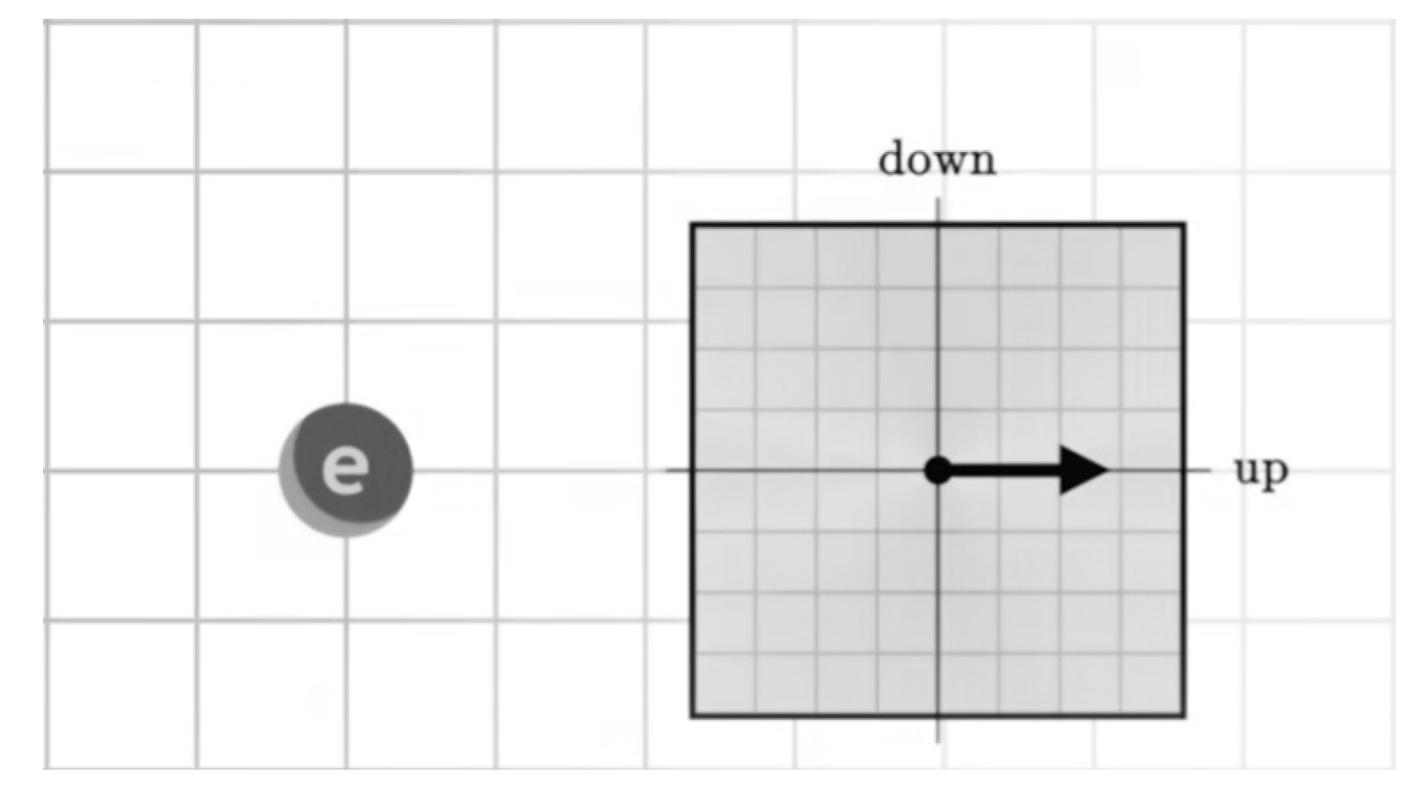
Figure 2.
On the left ,electron rotated (in this case intrinsic rotation is represented by physical rotation for easy of understanding) and on the right State space representation of rotation in Euclidian space.
Figure 2.
On the left ,electron rotated (in this case intrinsic rotation is represented by physical rotation for easy of understanding) and on the right State space representation of rotation in Euclidian space.
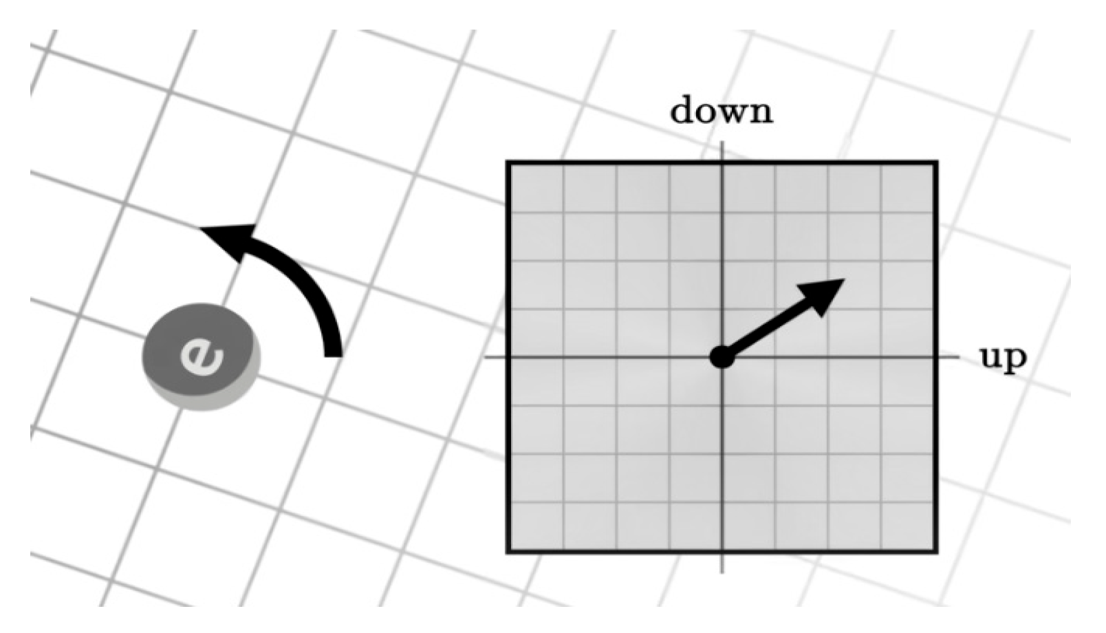
Figure 3.
Spin up electron becomes spin down after one half of a rotation (or a quarter rotation in Euclidean Space).
Figure 3.
Spin up electron becomes spin down after one half of a rotation (or a quarter rotation in Euclidean Space).
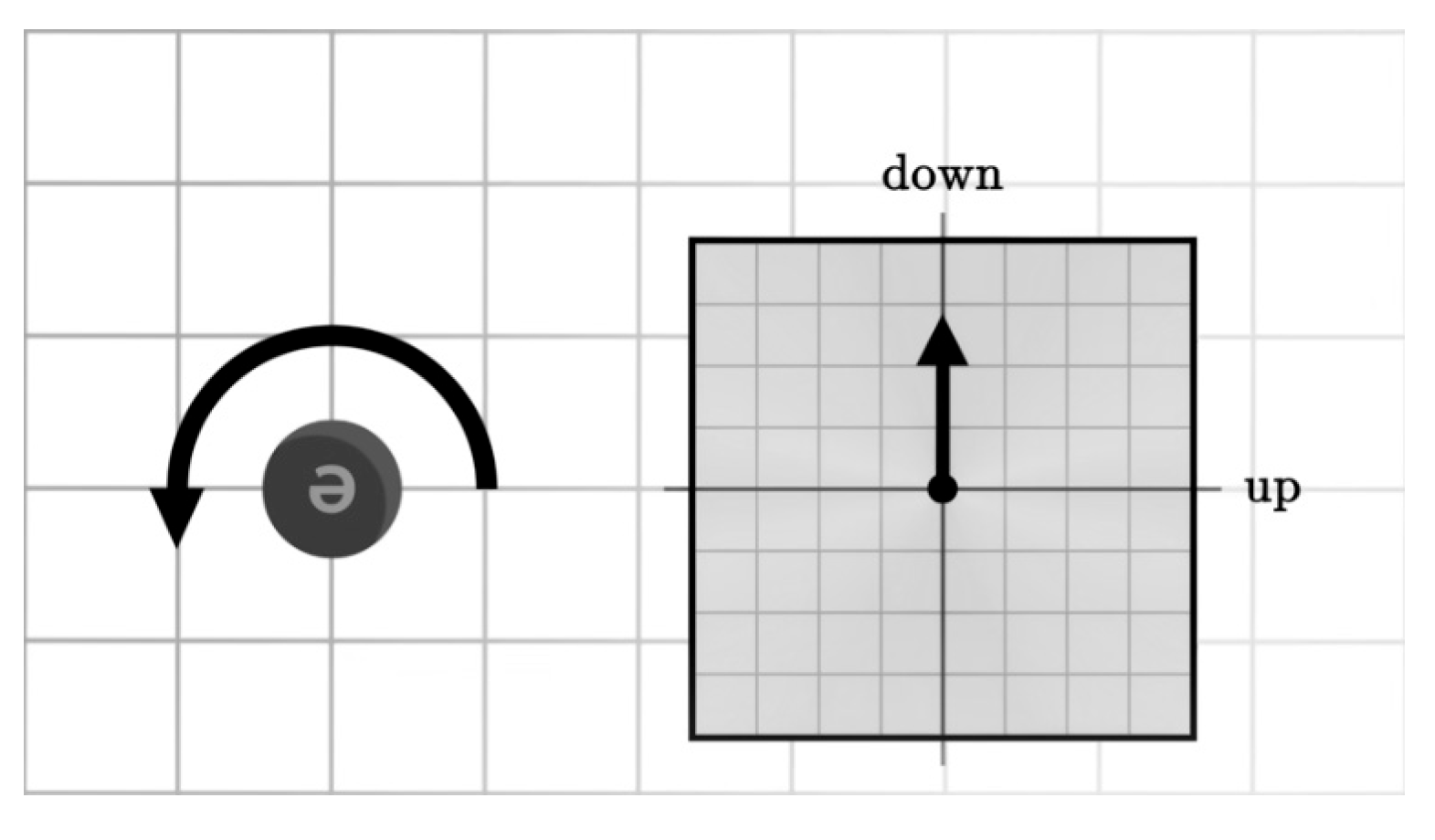
Figure 4.
After a full turn in actual space the electron has returned to its original position. However in Euclidean space the electron has only done through half a turn. For this reason it is called a spin particle.
Figure 4.
After a full turn in actual space the electron has returned to its original position. However in Euclidean space the electron has only done through half a turn. For this reason it is called a spin particle.
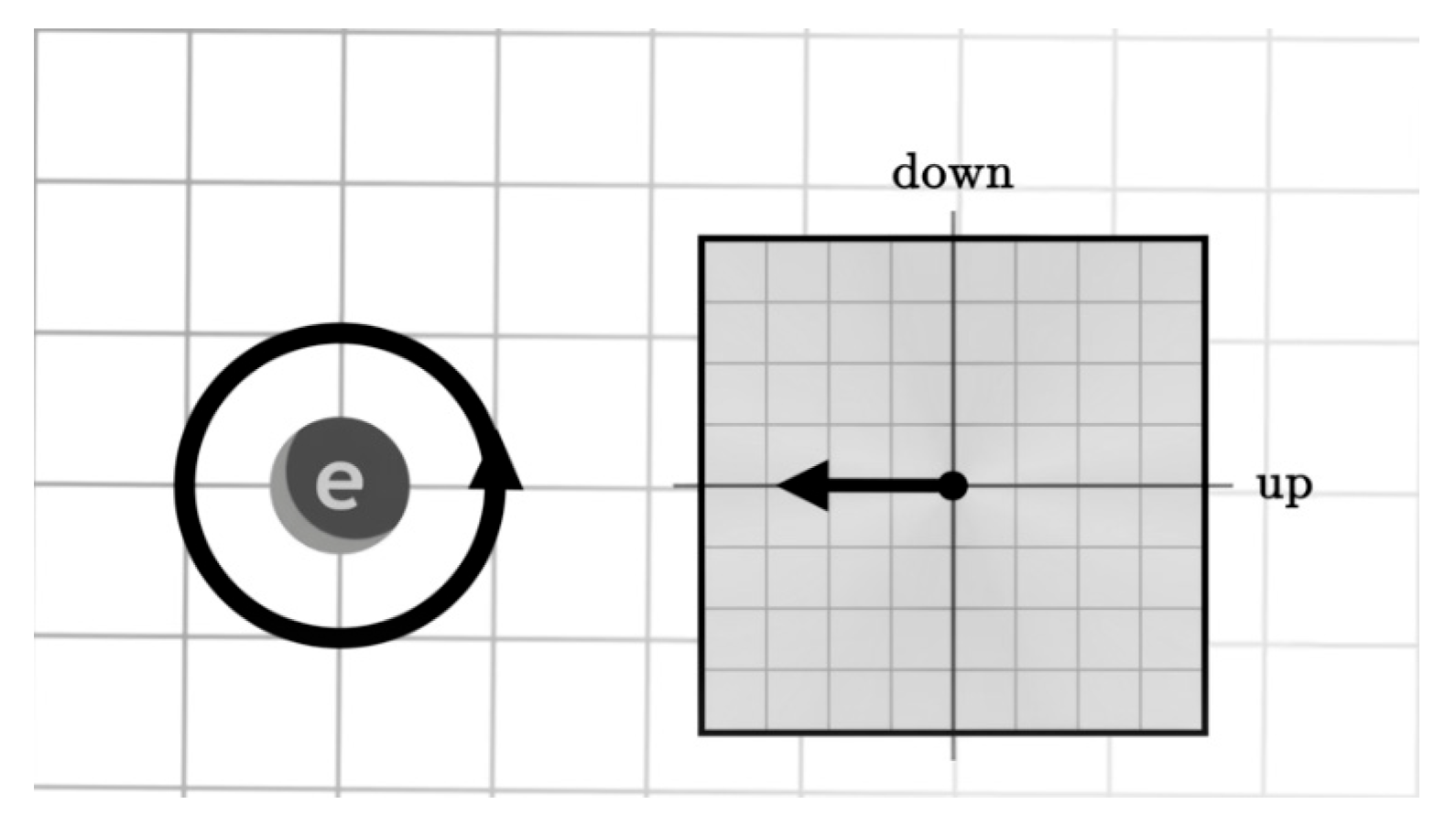
Figure 5.
Depiction of evanescent (or decaying) wave.
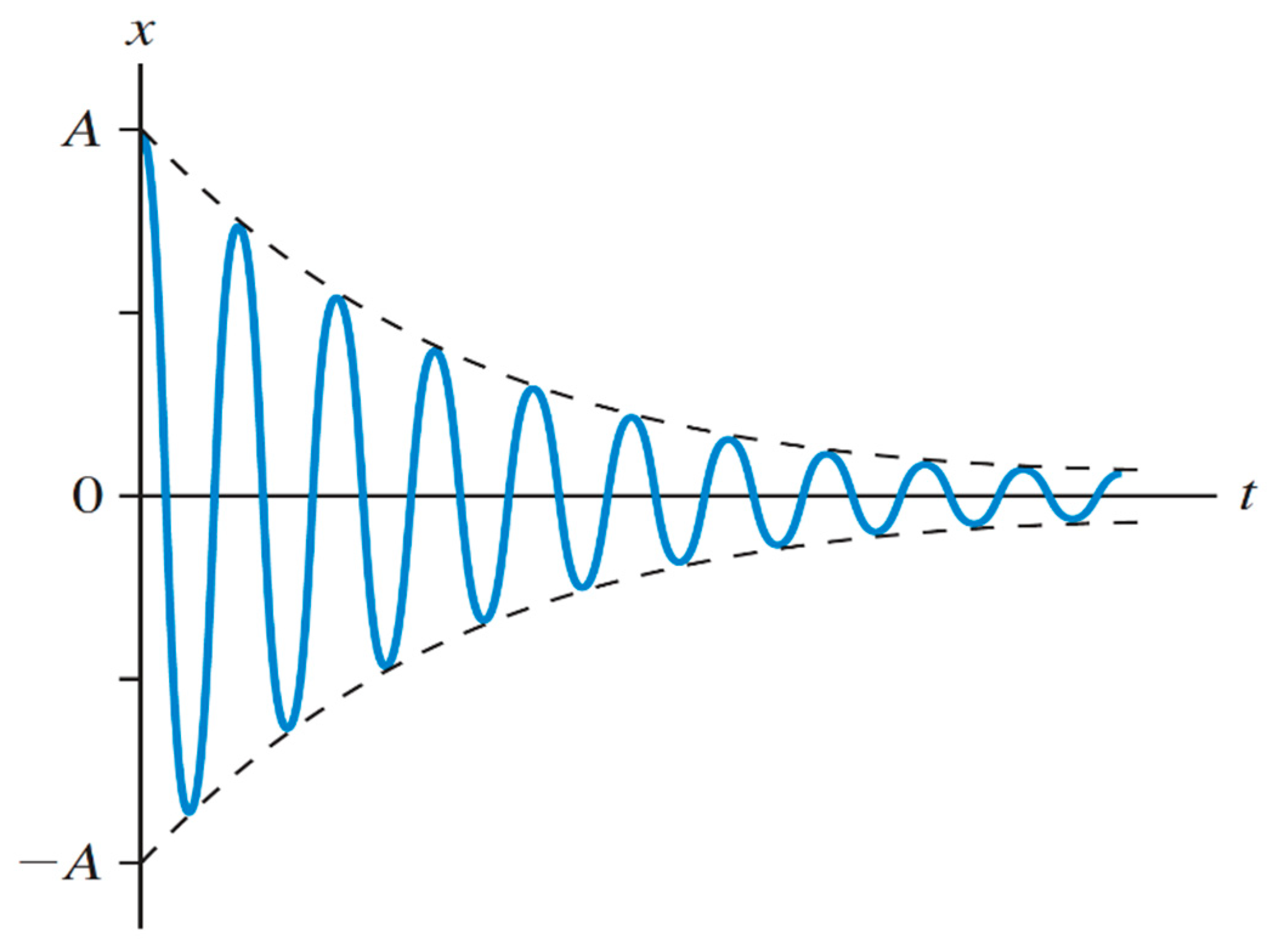
Figure 6.
Types of Dampening.
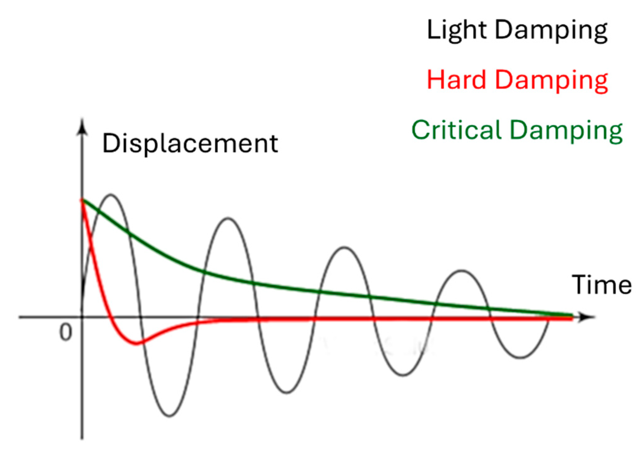
Figure 7.
The procedure for applying the Semi-structured complex framework.
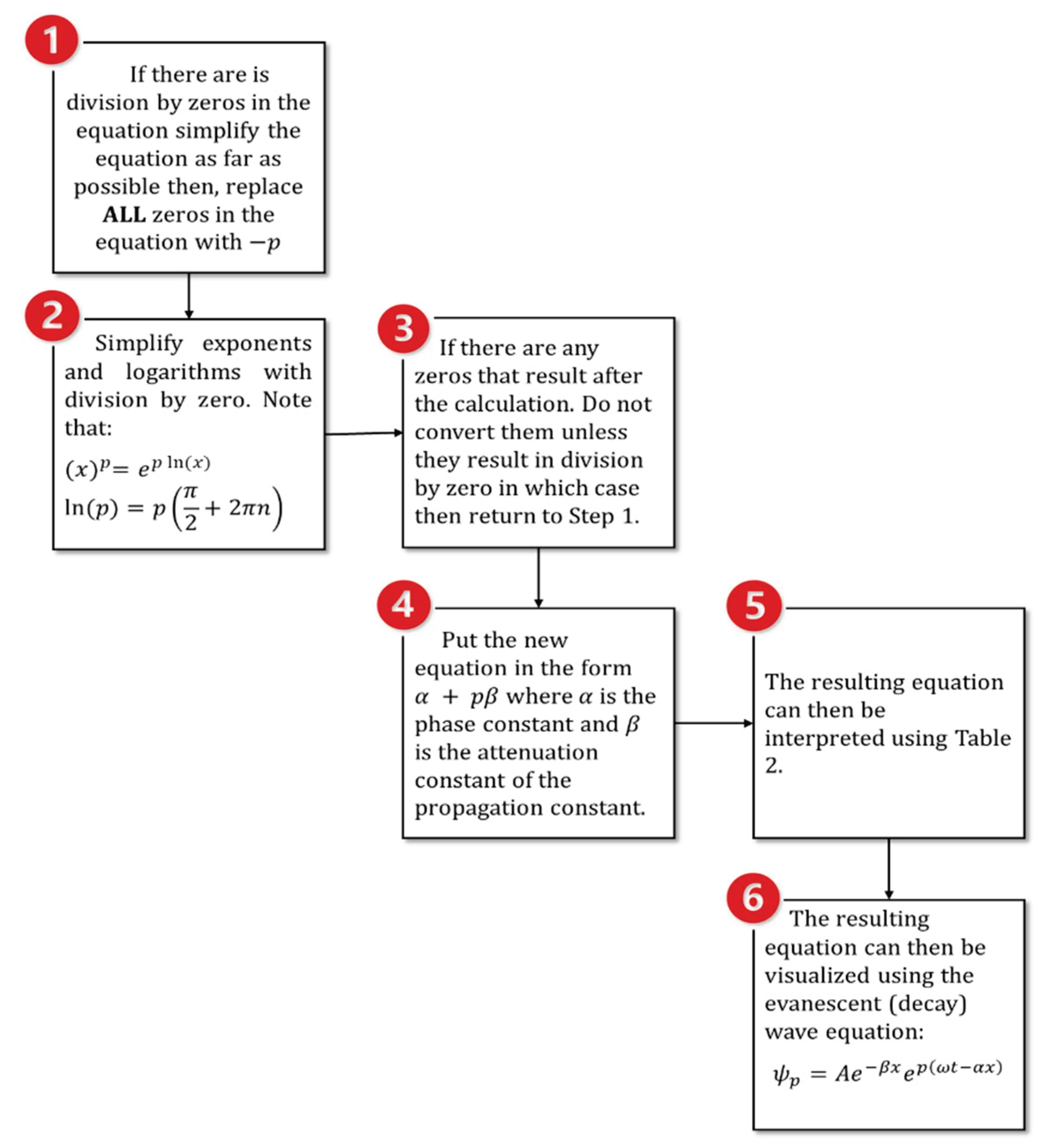
Figure 8.
One-loop scattering diagram.


Table 1.
Type of propagation constants and meaning.
| Damping Type | Equation form | Phase Constant | Attenuation Constant | Description |
|---|---|---|---|---|
| Undampened | The wave form does not experience damping but oscillates (and propagates) with a constant amplitude | |||
| Under-dampened | Waveform oscillates and decays slowly. | |||
| Critically Dampened | has a repeated root | Wave form does not oscillate but decays very quickly returning to equilibrium as quickly as possible without oscillating | ||
| Over-dampened (hard dampening) | has two distinct root | Waveform does not oscillate the system has more damping than critical, so it returns to equilibrium slowly and without oscillation. |
Table 2.
Type of propagation constants and meaning.
| Damping Type | Equation form | Phase Constant | Attenuation Constant | Description |
|---|---|---|---|---|
| Undampened | The wave form does not experience damping but oscillates (and propagates) with a constant amplitude | |||
| Underdampened | Waveform oscillates and decays slowly. | |||
| Critically Dampened | has a repeated root | Wave form does not oscillate but decays very quickly returning to equilibrium as quickly as possible without oscillating | ||
| Overdampened (hard dampening) | has two distinct root | Waveform does not oscillate the system has more damping than critical, so it returns to equilibrium slowly and without oscillation. |
Table 3.
Major results from paper.
| Result 1 | Semi-structured complex number set can be defined as follows:A semi-structured complex number is a three-dimensional number of the general form that is, a linear combination of real (), imaginary () and unstructured () units whose coefficients are real numbers. . |
| Result 2 | The unstructured number was redefined as: (35)where is a composite function such that .Integer powers of yield the following cyclic results: |
| (35) | |
| Result 3 | ). |
| Result 4 | The field of semi-structured complex numbers was defined, and proof was given that this field obeys the field axioms. This implies (1) the number set can easily be used in everyday algebraic expressions and can be used to solve algebraic problems, (2) the number set can be used to form more complicated structures such as vector spaces and hence solve more complex problems that may involve “division by zero”. |
| Result 5 | does not form an ordered field. For the objects in a field to have an order, operations such as greater than or less than can be applied to these objects. This is because in an ordered field the square of any non-zero number is greater than 0; this is not the case with semi-structured complex numbers. |
| Result 6 | Semi-structured complex numbers can be represented by points in a 3-dimensional Euclidean -space. The xyz-space consist of three perpendicular axes: the real -axis, the imaginary y-axis, and the unstructured -axis. These axes form three perpendicular planes: the real-imaginary -plane, the real-unstructured -plane, and the imaginary-unstructured -plane. |
| Result 7 | was used to find a viable solution to the logarithm of zero. The logarithm of zero was found to be: (36)where k is some integer value. |
| (36) | |
| Result 8 | The new definition of provided an unambiguous understanding that simply represents clockwise rotation of the vector from the positive unstructured z-axis to on the positive real x-axis along the real-unstructured -plane. Note that is any real number. |
| Result 9 | Semi-structured complex numbers have both a 3D and 4D representation in the form: (3D form) (4D form)are semi-structured basis units. |
| (3D form) | |
| (4D form) | |
| Result 10 | Two new Euler formulas were developed. 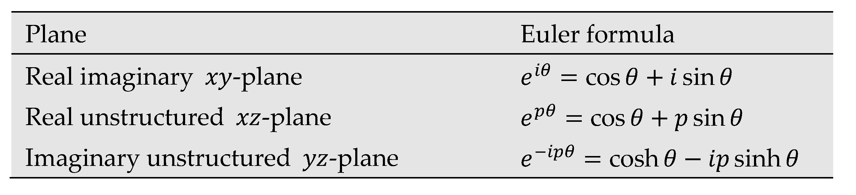 When combined with the original Euler formula describes the relationship between trigonometric, hyperbolic, and exponential functions for the entire semi-structured complex Euclidean -space. When combined with the original Euler formula describes the relationship between trigonometric, hyperbolic, and exponential functions for the entire semi-structured complex Euclidean -space. |
| Plane | Euler formula |
| -plane | |
| -plane | |
| -plane | |
| Result 11 | Semi-structured complex numbers can be used to resolve singularities that may arise in engineering and science equations (because of division by zero) to develop reasonable conclusions in the absence of experimental data. |
| Result 12 | From Result 10 semi-structured complex numbers can present in four forms as given below: 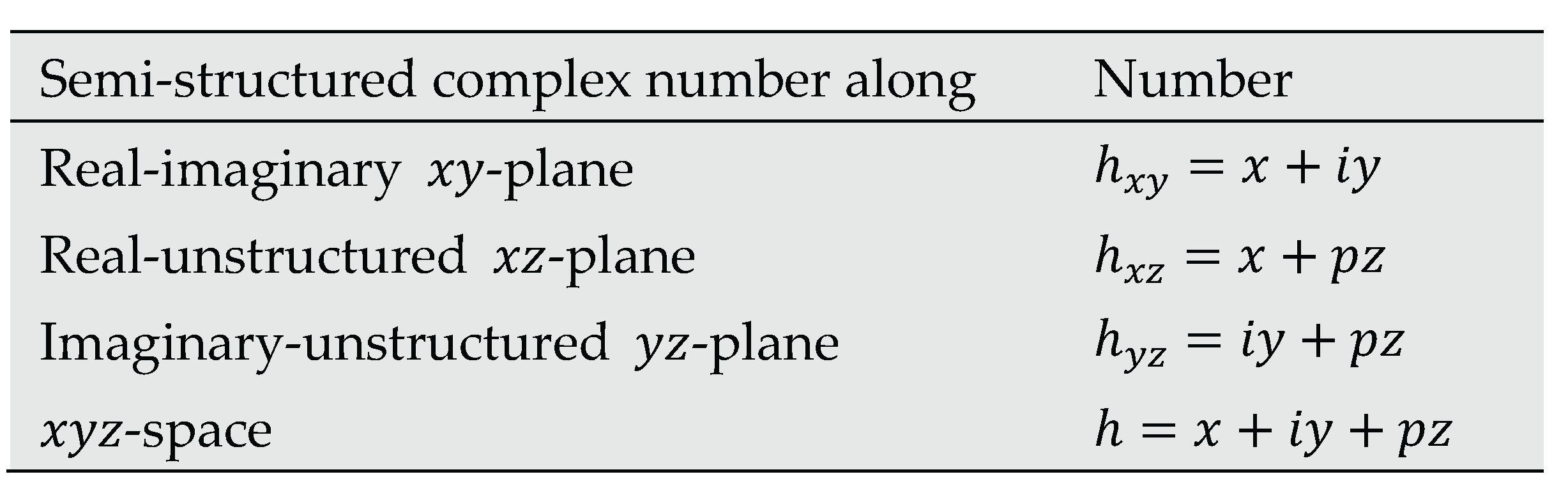 |
| Semi-structured complex number along | Number |
| -plane | |
| -plane | |
| -plane | |
| -space | |
| Result 13 | The zeroth root of a number h can be found using the equation |
| Result 14 | Since this implies that which further implies that |
| Result 15 | can be calculated given enough information) |
| Result 16 | If and measure different (but quantitatively related) aspects of the same object, where is physically measurable but is not, then and can be combined into one equation in the form |
Table 4.
Properties of P-algebra.
| Conjugation: |
Disclaimer/Publisher’s Note: The statements, opinions and data contained in all publications are solely those of the individual author(s) and contributor(s) and not of MDPI and/or the editor(s). MDPI and/or the editor(s) disclaim responsibility for any injury to people or property resulting from any ideas, methods, instructions or products referred to in the content. |
© 2025 by the authors. Licensee MDPI, Basel, Switzerland. This article is an open access article distributed under the terms and conditions of the Creative Commons Attribution (CC BY) license (http://creativecommons.org/licenses/by/4.0/).
Copyright: This open access article is published under a Creative Commons CC BY 4.0 license, which permit the free download, distribution, and reuse, provided that the author and preprint are cited in any reuse.


