Submitted:
05 June 2025
Posted:
06 June 2025
You are already at the latest version
Abstract
Using molecular dynamics simulations, we reveal how confinement in armchair MoS2 nanotubes alters the stability and melting points of hexagonal ice clusters. Ordered and hydrogen-disordered ice is studied inside and between nanotubes, showing a 30 K upward melting point shift for disordered interstitial ice due to hydrogen bond defects. The effects of nanotube diameter and ice impurities are quantified, highlighting MoS2’s potential in modulating phase transitions for applications in cryobiology and materials science.
Keywords:
Molybdenum disulfide (MoS2)
; ice
; nanoconfined
; constrained melting
; hydrogen‐defects
; Gibbs‐Thomson effec
1. Introduction
As is well-known, the behavior of materials in the bulk phase differs considerably from their behavior at the nanoscale [1] due, at least, to the dominance of surface/edge effects given the much larger surface/volume ratio at the nanoscale. Confining matter into a nanoscale cavity allows one to fine-tune several properties [2], as is often done [3], with applications in biology [4,5], Li-ion batteries [6,7], and other fields [8,9,10]. The confinement of water and/or ice and how this can modulate their properties, the subject of this study, is of fundamental and applied interest [11,12]. Solid water, i.e., ice, is the subject of this study [13,14] as a confined material [3,15,16,17]. Ice has many phases [18,19] with a few stable structures, including a ubiquitous one with hexagonal unit cells [14,16,20,21], which this work considers. The effect of ice crystals’ confinement in a nano environment is investigated, focusing on the melting point, which is among a material’s prime characteristics [22]. The factors affecting the melting process at the nanoscale [23] constitute the focal point of this work.
The behavior of confined nanoscale materials is known to depend on the volume of confinement. In this work, this volume is controlled by adjusting the diameter of the confining nanotube, as several other researchers have recently done in different contexts [24,25]. For example, Zheng et al. [26] use MD simulations to investigate the dependence of the diffusion mechanism on the diameter of a confining nanotube, while Erko et al. [27], using Raman scattering, find that decreasing the nanotube size caused significant changes in the core part of the confined water. Other investigations have explored the relation between the diameter of the confining nanotube and properties such as the boiling temperature of confined water nanodroplets [28], static properties of confined water [29], the heat of desorption [15], the density of water [26,30], surface tension [15], and the hydrogen-bonded network [30,31]. In addition to the confinement size, the nanotube material itself has a role in determining the behavior of confined ice. A type of nanotube that has sparked much recent interest is that of MoS₂, which possesses relatively low thermal conductivity compared to carbon nanotubes and, in some respects, may be considered an alternative to carbon nanotubes [32]. Several experimental and theoretical reports have studied these nanotubes’ physical properties, such as hardness [33,34], deformation during contact [33,34], and their uses in batteries [35,36] or as catalysts [37].
This paper uses molecular dynamics (MD) simulations to investigate the behavior of ice encapsulated within a set of packed MoS₂ nanotubes. The study examines the effect of MoS₂ nanotubes on the melting point of ice and explores how the arrangement of ice influences its melting point. Furthermore, the research investigates the impact of structural defects on the melting point, specifically hydrogen-disordered ice compared to hypothetical perfect hydrogen-ordered ice [38]. The important parameters this work determines are the melting points of various confined hexagonal ice nanocrystals in ordered and disordered forms. The effect of the size of the confining space is explored by repeating the calculations with nanotubes having two different diameters. The correlation between water and MoS₂ nanotubes offers a promising path for investigation within diverse scientific and technological fields.
2. Simulation Details
All simulations were performed using the software LAMMPS Molecular Dynamics Simulator. The materials are made using GenIce [38,39]. GenIce is an efficient algorithm written in Python 3 for generating ice structures with hydrogen disorder. Periodic boundary conditions (PBC) have been imposed to repeat the cells and infinitum. Two models of hexagonal ice are examined: An order crystal and one with irregularities and defects introduced by altering the number of hydrogen atoms. This software randomizes the hydrogen atoms in the ice, obeying the basic structural constraints and maintaining the cluster's overall charge neutrality. The NPT ensemble has been implemented in all calculations. Simulation times were modified by changing the heating rate value. The PPPM method is a computational method used in MD simulations to calculate long-range electrostatic interactions efficiently [40]. Two types of potential were used to model non-bonded dispersion interactions. The first is Lenard-Jones (LJ) 12-6 potential [41,42]. The LJ potential has been used for ice and its interactions with nanotubes. The second is the reactive empirical bond-order (or REBO) many-body potential, which we used to describe the Mo-S interactions [36]. It is a bond order potential as an empirical potential energy function used in molecular dynamics simulation to model interactions between atoms in a system. Unlike traditional forcefields, which typically use fixed bond orders and bond lengths, this one considers varying ones. Further, a reactive part is used to account for bond-making and breaking during MD simulations. Combining these force fields can produce a specific type of potential energy function designed to model reactive behavior and bond changes accurately. This potential is known for its predictive ability of chemical reactions and mechanical and thermal properties of materials [36,43,44]. Ahadi et al. [36] describe the analytical form of this potential, while Maździarz [45] has demonstrated its suitability to model MoS2 by comparing its predictions with those of density functional theory (DFT) calculations. These are the rationales for our choice of this potential to study the stability and thermal properties of MoS2 nanotubes with the inter-atomic potential parameters listed in Table 1 a) and b). The effective charges for oxygen and hydrogen are taken (in atomic units (a.u.), i.e., as |e|=1 as -1.1794 and +0.5897, respectively [46]. The mean pressure was kept at about 1 bar during the simulations using a Nose-Hoover thermostat. The time step for all simulations is 0.001 ps (1 fs) and run times are 1 ns to 2 ns depending on heating rate. In addition, Table 2 shows states, nanotube types, the number of water molecules, and CPU time.

Table 1.
a) Lenard Jones potential parameters [35].
Table 1.
a) Lenard Jones potential parameters [35].
| Interaction | ε (eV) | σ (Å) |
| H-O | 0.0 | 0.0 |
| O-O | 0.00914 | 3.1668 |
| H-H | 0.0 | 0.0 |
| H-Mo | 0.0 | 0.0 |
| H-S | 0.0 | 0.0 |
| O-Mo | 0.002314 | 3.6834 |
| O-S | 0.011255 | 3.1484 |
Table 1.
b) REBO potential parameters [36].
Table 1.
b) REBO potential parameters [36].
| Interaction | Q | (Å) | A | B | β |
| Mo-Mo | 3.4191 | 179.0080 | 1.0750 | 716.9465 | 1.1610 |
| Mo-S | 1.5055 | 575.5097 | 1.1927 | 1344.4682 | 1.2697 |
| S-S | 0.2550 | 1228.4323 | 1.1078 | 1500.2125 | 1.1267 |
| state | Nanotube type |
Nanotube total atoms |
x(Å) | y(Å) | z(Å) | Water molecules |
CPU Time/hrs |
| Order-inside | (22,22) | 5643 | 141.4 | 141.4 | 48.9 | 1174 | 205 (rate 0.13) |
| Order-outside | (22,22) | 45633 | 108.6 | 109.4 | 44.4 | 14595 | 236 (rate 0.13) |
| Disorder-inside | (22,22) | 4971 | 141.4 | 141.8 | 42.6 | 1041 | 195 (rate 0.13) |
| Disorder-outside | (22,22) | 33477 | 90.5 | 94.1 | 48.9 | 10455 | 370 (rate 0.13) |
3. Results and Discussion
For simulating dynamic processes such as melting and examining structural changes with proper time resolution, it is more appropriate to use the molecular dynamics method, as it can simulate molecular behaviors more accurately, as demonstrated in studies such as Karim et al. [47]. The effect of two confinement modes on the melting temperature has been considered. One is where the water fills the interstices between the nanotubes, leaving the interiors of the tubes empty, and the second fills the interiors of the nanotubes with water molecules, leaving the interstices empty. The two systems considered are illustrated in Figure 1. In all cases, the initial ice structure is hexagonal, whether in “order” or “hydrogen-defective” cases.
3.1. Structural Stability
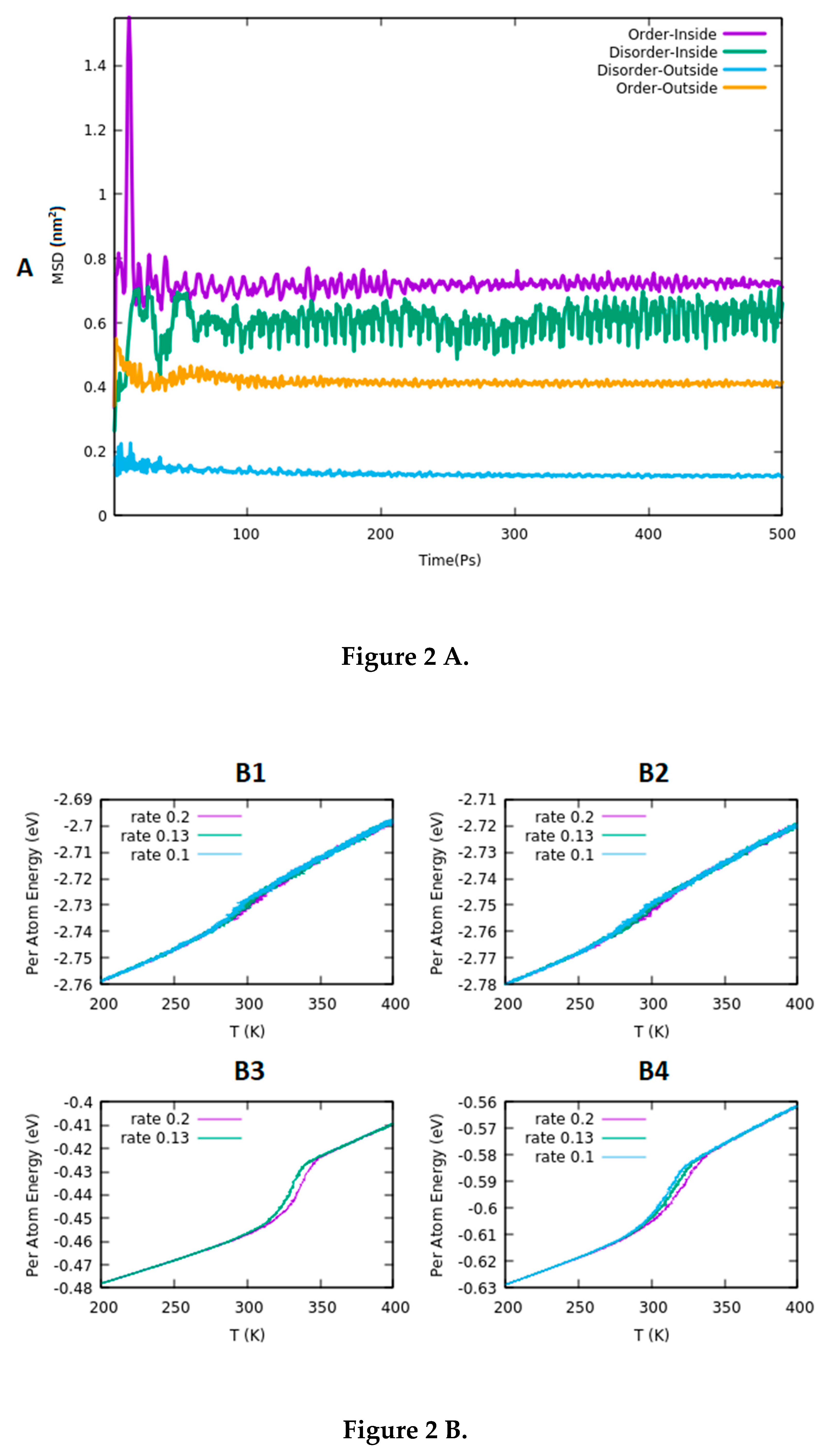
Figure 2a displays the variation of mean square displacement (MSD) as a function of time for four states of confined ice, the arrangements of which are exhibited in Figure 1. In a stable system, particles tend to remain localized around their initial positions or within a confined region. For all states, the figure suggests the temporal stability of the system under study since the patterns appear stable (after ca. 50 ps of initial strong fluctuations) within the remainder of the 500 ps of the simulation. As can be seen, the MSD exhibits relatively flat or plateau-like behavior at longer time scales. This plateau indicates that the displacements of the particles remain limited, with no significant diffusion over time.
3.2. Determination of the Melting Point
The time rate of heating, i.e., power (W = dQ/dt), and its accompanying temperature increase (dT/dt) is important to control in MD studies of melting points. It should be noted that the time rate of heating can control reaction kinetics, phase transitions, and the behavior of materials. Figure 2b shows that three different powers (heating rates) were tested. The results suggest that the slower heating rate produces significant results compared to other ones (higher rates, 0.13 and 0.2) on the structures of crystalline water ice.
The (22, 22) MoS2 nanotube with a diameter of about 66.36 Å was selected first. For this system, Figure 2b displays the energy per atom as a function of the temperature at three different powers. The results suggest a clear phase transition occurs when ice fills the interstices between the nanotubes (plots b3 and b4), as evidenced by the dramatic slope changes. Fernández et al. find that hydrogen-disordered ice melts at a higher temperature than in its order state by ca. 20◦C [48]. These researchers [48] report observing extreme phase transition temperatures of water confined inside isolated carbon nanotubes. In contrast, our results suggest that when ice is inside the MoS2 nanotube, this phase transition is washed out, and the difference between the two ice models (order and disordered) is not distinguishable. In the latter case, both ice structures melt gradually in the range of ca. 280 to 310 K. It can be concluded that confinement causes a dramatic change in the melting behavior of ice, which can perhaps be exploited in future fundamental or applied work due to the importance of ice melting point in the environment. Further, it is noted that reducing the heating rate is accompanied by a marked decrease in the melting temperature range of ice. This is especially visible when ice has the disorder. Since the results obtained from the temperature rate of heating 0.1 K. PS-1 exhibit the best agreement with experimental data, this heating rate will be used subsequently.
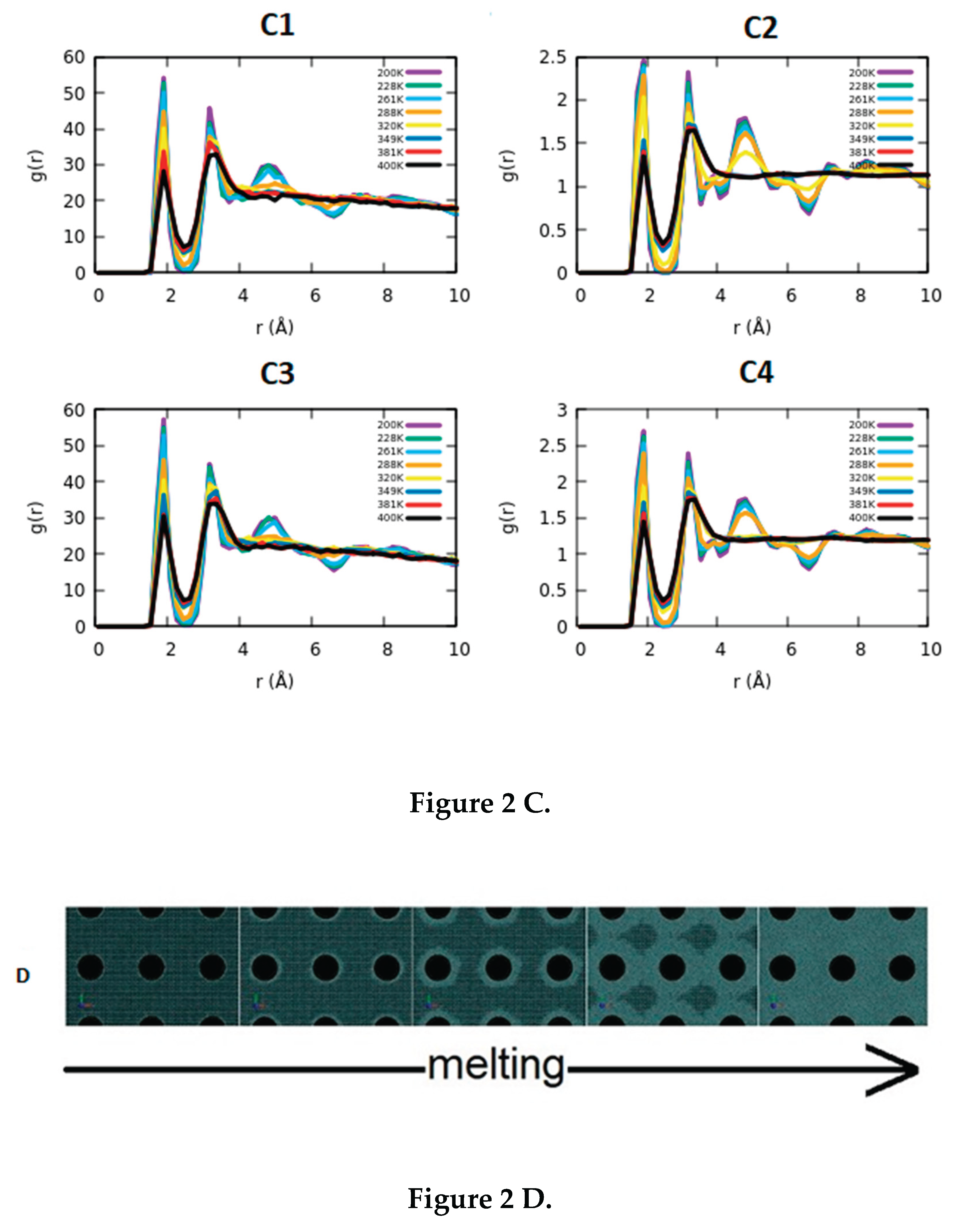
Figure 2c compares the radial distribution function (RDF) at different temperatures. This diagram shows the transition from solid to liquid in various colors. The plots of the RDF in Figure 2c are consistent with the heating curves in Figure 2b. In the state where ice is confined inside the nanotubes, there is not much difference between ordered ice and the hydrogen-defective (disordered), and both start to melt at about 288 K. However, the difference is significant when ice is confined between the MoS2 nanotubes. For hydrogen-defect-free ice, it starts to melt after 288 K and is completely melted at 320 K. However, in the case of ice with hydrogen defects, melting happens at higher temperatures, starting at approximately 320 K. This upward shift of the melting point of water by about 30 K can lead to industrial exploitation. Potential industrial applications stemming from controlling water’s phase behavior include cryobiology, cryosurgery, food processing, thermal energy storage, phase change materials, the pharmaceutical industry, and materials science[49,50,51] . For the MoS2 nanotube of (9,9) (with a diameter of about 18.7 Å), the energy per atom is plotted in Figure 3a. In contrast, the corresponding RDF plots are given in Figure 3b. The focus here is on the state of interstitial ice since it has an interesting phase transition worthy of a closer examination. There appears to be no significant difference in the phase transition in response to changing the radii of the nanotubes from (22,22) to (9,9). A slight difference (of only a few degrees) is found between the two radial distribution functions, indicating that reducing the confinement radius when ice exists in the outer interstitial space and trapped between the MoS2 nanotubes has negligible effect on the melting point.
The Gibbs-Thomson effect is a thermodynamic phenomenon that describes how the equilibrium properties of a phase transition, such as melting and freezing, are influenced by the size of particles or droplets. Specifically, it states that smaller crystals or droplets exhibit a lower melting temperature (or higher freezing temperature) than their larger counterparts due to the increased curvature at their surfaces, resulting in elevated interfacial energy. This heightened energy requirement for smaller structures increases chemical potential, necessitating different equilibrium conditions than those experienced by bulk materials. In confined geometries—such as liquids trapped within porous media—the effect becomes even more pronounced; as pore sizes decrease, the curvature increases, causing significant reductions in melting and freezing temperatures. The implications of this phenomenon are critical across various fields, including materials science, nanotechnology, and geology. Understanding how confinement influences phase behavior can lead to advancements in material design and practical applications like cryopreservation or enhanced oil recovery techniques [52,53,54]. Based on our investigations, the absence of physical ice or real MoS2 in our molecular dynamics simulations, which solely utilize Lennard-Jones and REBO potentials, allows us to neglect the Gibbs-Thomson effect since it is not applicable under these conditions.
Figure 3.
(a) Energy per atom as a function of temperature for two different radii: (9,9) and (22,22). (b) RDFs of the two different radii, respectively.
Figure 3.
(a) Energy per atom as a function of temperature for two different radii: (9,9) and (22,22). (b) RDFs of the two different radii, respectively.
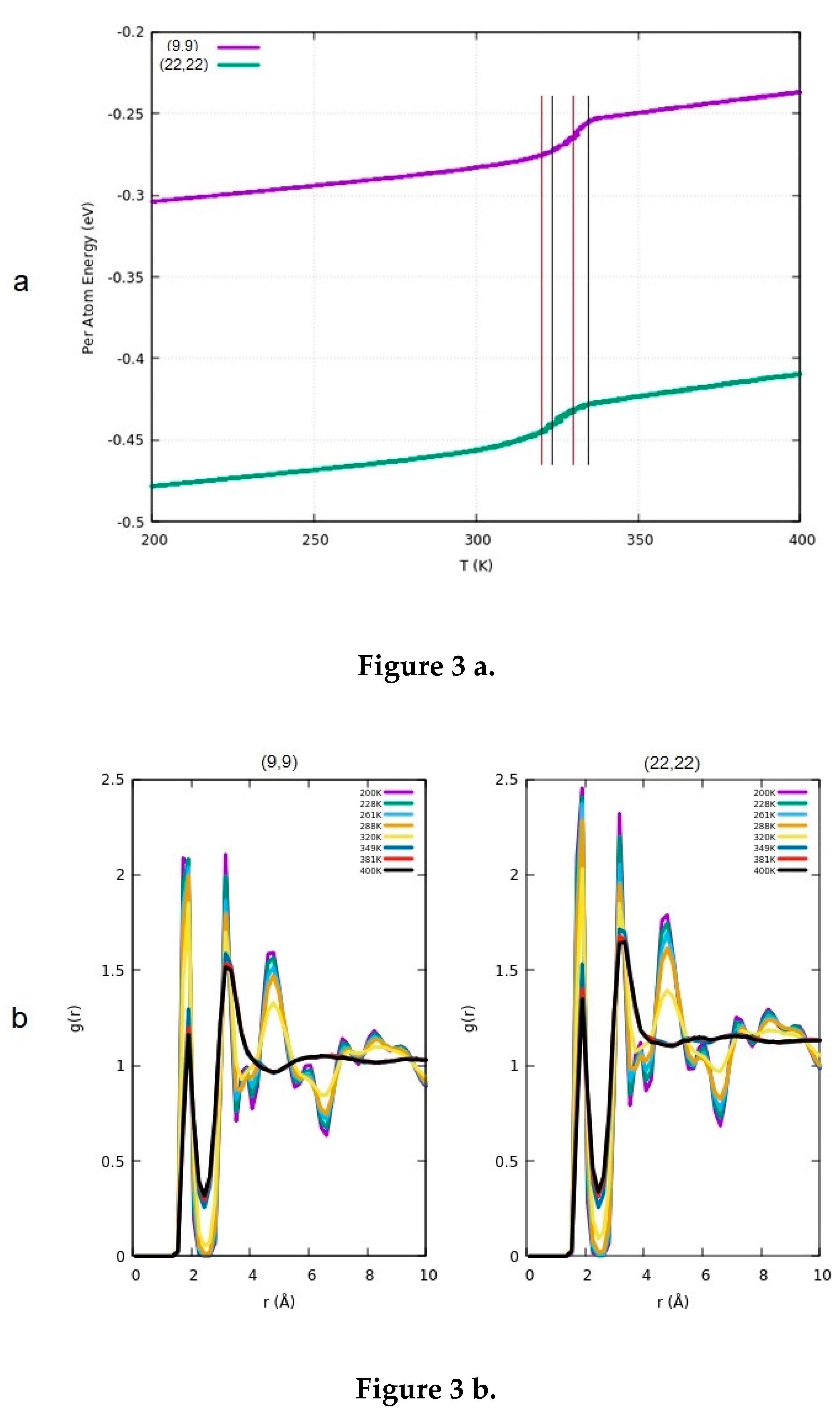
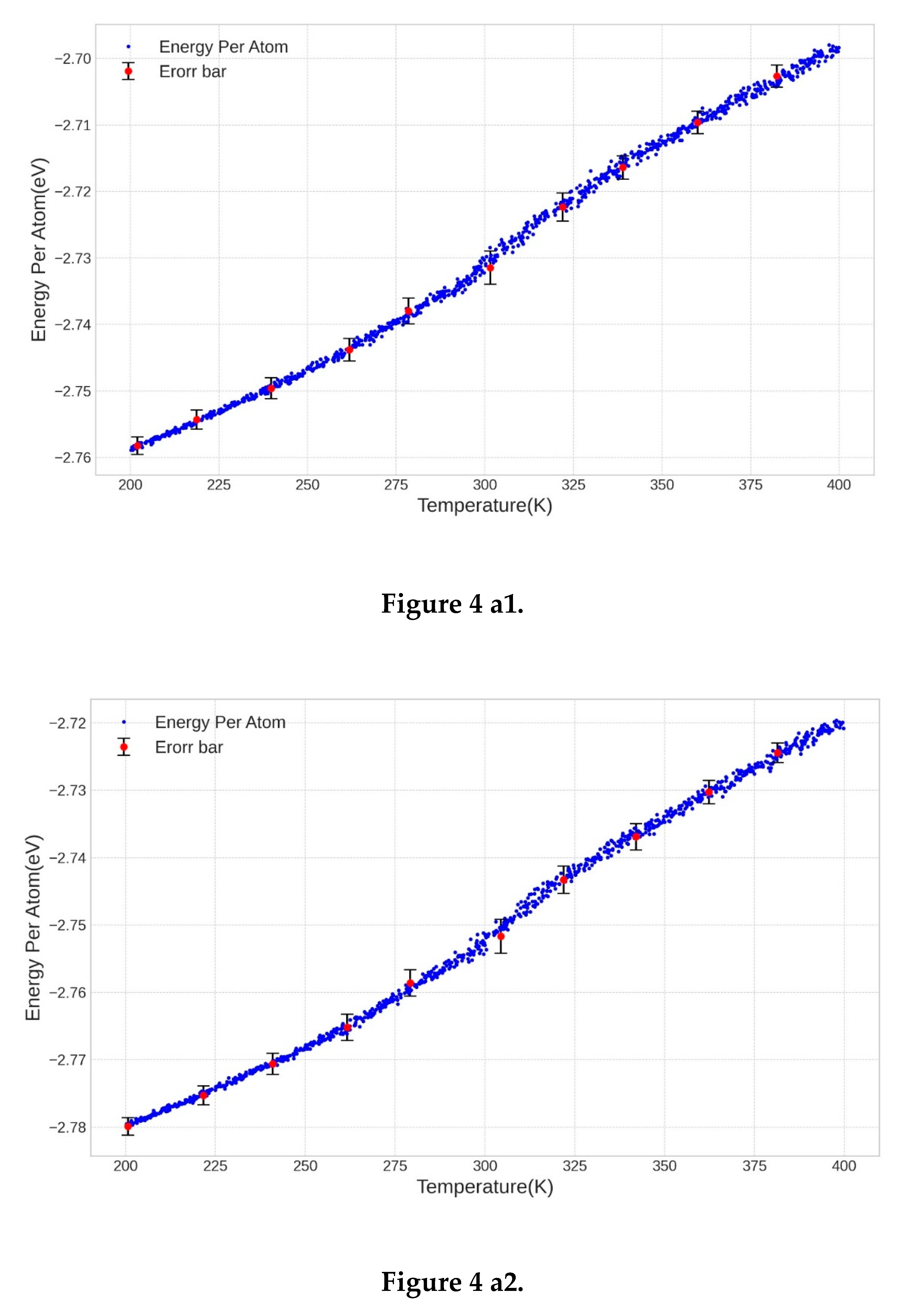
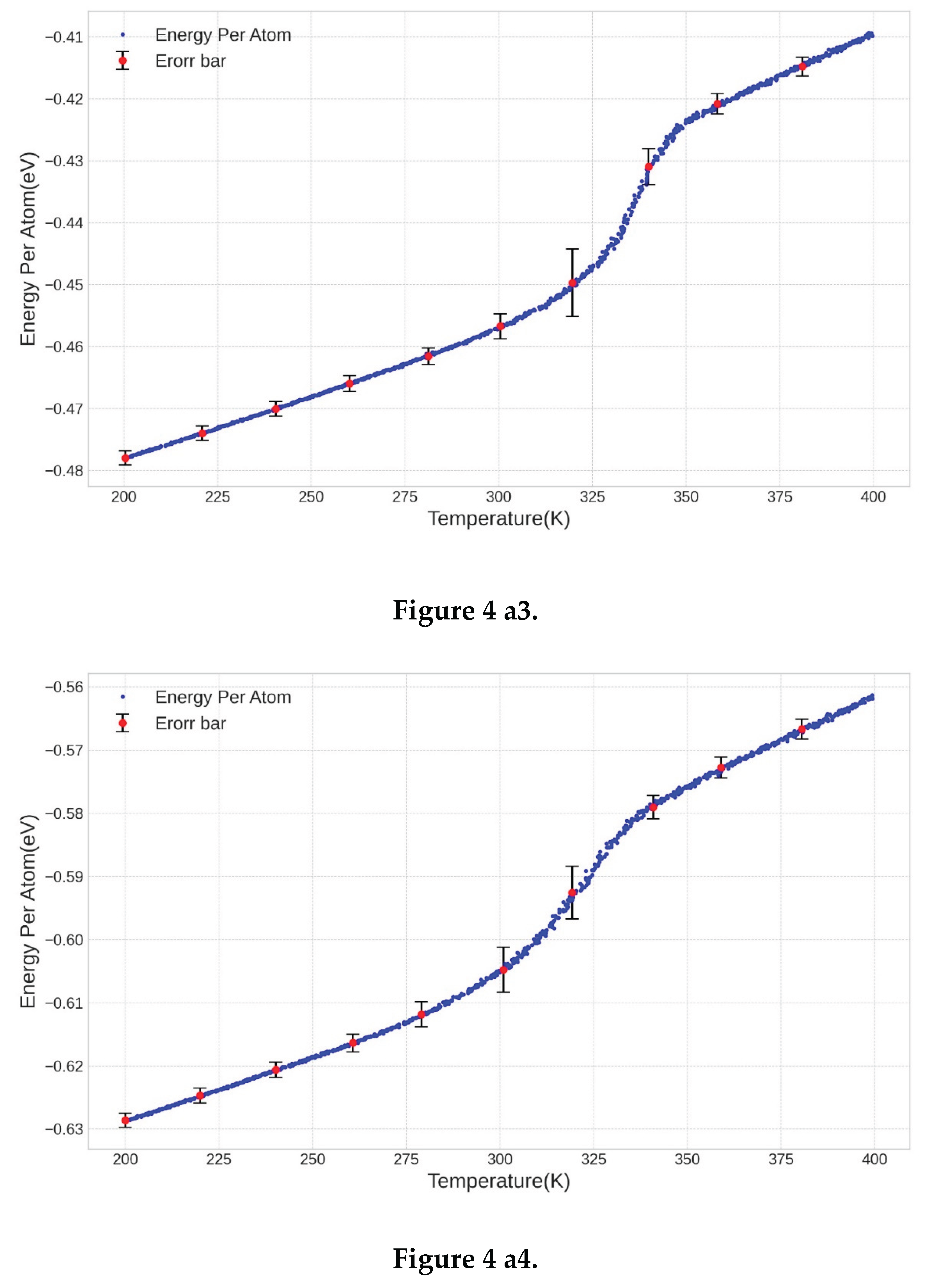
Figure 4.
It is a Figure 2B with error bars for heating rate equal to 0.2. a1 depicts a disordered hexagonal ice confined within a nanotube, a2 depicts an ordered hexagonal ice confined within a nanotube, a3 illustrates a disordered hexagonal ice surrounding the nanotube, and a4 illustrates an ordered hexagonal ice surrounding the nanotube.
3.3. Comparison of the Results
When comparing carbon nanotubes and MoS2 nanotubes, as utilized in this paper, it becomes apparent that the shift in the melting point can also be attributed to the material properties of the nanotubes. Specifically, the interaction between water molecules and the nanotube walls differs between these two substances. For CNTs, the material is nonpolar and hydrophobic, while MoS2 is hydrophilic and relatively more polar. In the case of CNTs, water exhibits lower adhesion to the walls, allowing molecules to move more freely, resulting in a delayed formation of an ordered structure, which in turn lowers the melting point. Additionally, the structural and energy levels differ between the two materials. In MoS2 nanotubes, the presence of S and Mo with relative charges leads to electrostatic effects on the water molecules. In contrast, such effects are absent in CNTs. Furthermore, the effect of spatial confinement and the radius of the tubes must be considered. Even if the tube radii are the same, the atomic layer arrangement differs between the two materials, resulting in a slight variation in the internal space that influences the arrangement of water molecules. All of these factors can contribute to the observed shift in the melting point. In comparing the Gibbs-Thomson effect for both CNTs and MoS2 nanotubes, we find that the change in the melting temperature due to this effect is a decrease of approximately 1.15K for CNTs and a decrease of about 2.21K for MoS2 nanotubes. This Comparison reveals that materials with higher surface energy and more complex structures exhibit a more substantial Gibbs-Thomson effect, resulting in greater changes in melting temperature compared to materials with lower surface energy and simpler structures. Table 3 shows a brief comparison of the results based on references.
Table 3.
Comparison of the results.
| Property | CNT | MoS2 nanotubes | CNT and Graphene | Graphene slit nanopores | CNT | CNT | CNT |
|---|---|---|---|---|---|---|---|
| Surface type | Hydrophobic (non-polar) | Hydrophilic (Semi-polar) | Hydrophobic | Hydrophobic | Hydrophobic | Hydrophobic | Hydrophobic |
| Interaction with water | Week | Moderate to strong | strong | Moderate to strong | strong | strong | strong |
| Melting point of confined water | Lower (~ -20˚C or less) | Higher (~ +10˚C or more) | Higher | - | Higher | Lower | - |
| Ice structure inside tubes | Irregular or ice nanotubes | More ordered, closer to known ice phases | ordered | amorphous | ordered | - | - |
| Water permeability | high | lower | high | lower | lower | - | high |
| Ice stability | Unstable at higher temperatures | More stable compared to CNT | Stable | Stable | Stable | - | - |
| Key References | [55] | [32] | [22] | [14] | [25] | [28] | [29] |
4. Conclusions
By introducing disorder in the ice and by varying its confinement status, it is found that ice melts to a greater extent in the disorder system than in order one. This occurs in ice placed in the interstices between the MoS2 nanotubes rather than inside them. When the ice surrounds the nanotubes, this may be regarded as adding an "impurity," which causes a significant upward shift in the melting point. This effect can be ascribed to a stronger interaction of the nanotube's surface with ice than the strength of the ice-ice (water-water) interaction. In the investigated case outside the (22,22) nanotube (between the nanotube area) and disorder system), this value is increased by about 30 degrees. Radius reduction of the nanotubes from (22,22) to (9,9), with interstitial disordered ice filling the space between the nanotubes, is accompanied by a reduction in melting temperature from 332 K to 338 K. A reduction in the temperature rate (dT/dt) is accompanied by a decrease in the ice melting range by about 20 K. This change is more pronounced when ice is disordered. These findings may lead to applications, such as the eventual development of high-temperature-resistant materials. The observed shift in the melting point between CNTs and MoS2 nanotubes can be attributed to differences in molecular interactions, structural properties, and spatial confinement, with CNTs exhibiting hydrophobic behavior and MoS2 nanotubes showing electrostatic effects on water molecules.
References
- F. Béguin, V. Pavlenko, P. Przygocki, M. Pawlyta, P. Ratajczak, Carbon 169 (2020) 501.
- K. Sotthewes, P. Bampoulis, H.J. Zandvliet, D. Lohse, B. Poelsema, ACS Nano 11 (2017) 12723.
- S. Chakraborty, H. Kumar, C. Dasgupta, P.K. Maiti, Acc. Chem. Res. 50 (2017) 2139.
- D. Han, X. Jin, Y. Li, W. He, X. Ai, Y. Yang, et al., J. Phys. Chem. Lett. 15 (2024) 2375.
- H.R. Corti, G.A. Appignanesi, M.C. Barbosa, J.R. Bordin, C. Calero, G. Camisasca, et al., Eur. Phys. J. E 44 (2021) 1.
- W. Wan, Z. Zhao, S. Liu, X. Hao, T.C. Hughes, J. Qiu, Nanoscale Adv. 6 (2024) 1643.
- A. Serva, N. Dubouis, A. Grimaud, M. Salanne, Acc. Chem. Res. 54 (2021) 1034.
- H. Zou, L. Yang, Z. Huang, Y. Dong, R.-Y. Dong, Int. J. Heat Mass Transf. 220 (2024) 124938.
- D. Dutta, T. Muthulakshmi, P. Maheshwari, Chem. Phys. Lett. 826 (2023) 140644.
- J.N. Bassis, A. Crawford, S.B. Kachuck, D.I. Benn, C. Walker, J. Millstein, et al., Annu. Rev. Earth Planet. Sci. 52 (2024).
- L. Salvati Manni, S. Assenza, M. Duss, J.J. Vallooran, F. Juranyi, S. Jurt, et al., Nat. Nanotechnol. 14 (2019) 609.
- I. Baranova, A. Angelova, W.E. Shepard, J. Andreasson, B. Angelov, J. Colloid Interface Sci. 634 (2023) 757.
- C.A. Angell, Annu. Rev. Phys. Chem. 55 (2004) 559.
- W.-H. Zhao, L. Wang, J. Bai, L.-F. Yuan, J. Yang, X.C. Zeng, Acc. Chem. Res. 47 (2014) 2505.
- A.W. Knight, N.G. Kalugin, E. Coker, A.G. Ilgen, Sci. Rep. 9 (2019) 8246.
- M. Jażdżewska, K. Domin, M. Śliwińska-Bartkowiak, A. Beskrovnyi, D.M. Chudoba, T. Nagorna, et al., J. Mol. Liq. 283 (2019) 167.
- T. Khan, M.-x. Han, X.-w. Kong, D. Qu, J.-l. Bai, Z.-q. Wang, et al., Chem. Phys. Lett. 856 (2024) 141666.
- A. Reinhardt, M. Bethkenhagen, F. Coppari, M. Millot, S. Hamel, B. Cheng, Nat. Commun. 13 (2022) 4707.
- S.L. Bore, F. Paesani, Nat. Commun. 14 (2023) 3349.
- J. Hayward, J. Reimers, J. Chem. Phys. 106 (1997) 1518.
- R. Ma, D. Cao, C. Zhu, Y. Tian, J. Peng, J. Guo, et al., Nature 577 (2020) 60.
- M. Raju, A. Van Duin, M. Ihme, Sci. Rep. 8 (2018) 3851.
- G. Wang, N. Wu, J. Wang, J. Shao, X. Zhu, X. Lu, L. Guo, RSC Adv. 6 (2016) 108343.
- S. Chiashi, Y. Saito, T. Kato, S. Konabe, S. Okada, T. Yamamoto, Y. Homma, ACS Nano 13 (2019) 1177.
- M. Matsumoto, T. Yagasaki, H. Tanaka, J. Chem. Phys. 154 (2021) 094702.
- Y.-g. Zheng, H.-f. Ye, Z.-q. Zhang, H.-w. Zhang, Phys. Chem. Chem. Phys. 14 (2012) 964.
- M. Erko, G.H. Findenegg, N. Cade, A. Michette, O. Paris, Phys. Rev. B 84 (2011) 104205.
- V.V. Chaban, V.V. Prezhdo, O.V. Prezhdo, ACS Nano 6 (2012) 2766.
- J. Wang, Y. Zhu, J. Zhou, X.-H. Lu, Phys. Chem. Chem. Phys. 6 (2004) 829.
- G. Cicero, J.C. Grossman, E. Schwegler, F. Gygi, G. Galli, J. Am. Chem. Soc. 130 (2008) 1871.
- M.K. Tripathy, D.K. Mahawar, K. Chandrakumar, J. Chem. Sci. 132 (2020) 1.
- P. Bampoulis, V.J. Teernstra, D. Lohse, H.J. Zandvliet, B. Poelsema, J. Phys. Chem. C 120 (2016) 27079.
- A.N. Enyashin, S. Gemming, M. Bar-Sadan, R. Popovitz-Biro, S.Y. Hong, Y. Prior, et al., Angew. Chem. Int. Ed. 46 (2007) 623.
- A.O. Pereira, C.R. Miranda, J. Phys. Chem. C 119 (2015) 4302.
- T. Stephenson, Z. Li, B. Olsen, D. Mitlin, Energy Environ. Sci. 7 (2014) 209.
- Z. Ahadi, M. Shadman Lakmehsari, S. Kumar Singh, J. Davoodi, J. Appl. Phys. 122 (2017) 224305.
- D. Maharaj, B. Bhushan, Sci. Rep. 5 (2015) 8539.
- M. Matsumoto, T. Yagasaki, H. Tanaka, J. Comput. Chem. 39 (2018) 2454.
- M. Matsumoto, T. Yagasaki, H. Tanaka, J. Chem. Inf. Model. 61 (2021) 2542.
- R.W. Hockney, J.W. Eastwood, Computer Simulation Using Particles, CRC Press, 2021.
- J.E. Jones, Proc. R. Soc. London, Ser. A 106 (1924) 441.
- J.E. Lennard-Jones, Proc. Phys. Soc. 43 (1931) 461.
- S. Xiong, G. Cao, Nanotechnology 27 (2016) 105701.
- B. Mortazavi, T. Rabczuk, RSC Adv. 7 (2017) 11135.
- M. Maździarz, Materials 14 (2021) 519.
- J. Abascal, E. Sanz, R. García Fernández, C. Vega, J. Chem. Phys. 122 (2005) 234511.
- O.A. Karim, A. Haymet, J. Chem. Phys. 89 (1988) 6889.
- R. García Fernández, J.L. Abascal, C. Vega, J. Chem. Phys. 124 (2006) 144506.
- T. Chang, G. Zhao, Adv. Sci. 8 (2021) 2002425.
- R.P. Bebartta, R. Sehrawat, K. Gul, Advances in Biopolymers for Food Science and Technology, Elsevier, 2024, p. 445.
- J.-R. Authelin, M.A. Rodrigues, S. Tchessalov, S.K. Singh, T. McCoy, S. Wang, E. Shalaev, J. Pharm. Sci. 109 (2020) 44.
- L. Scalfi, B. Coasne, B. Rotenberg, J. Chem. Phys. 154 (2021) 114708.
- J.W. Cahn, J.E. Hilliard, J. Chem. Phys. 28 (1958) 258.
- D.V. Svintradze, Biophys. J. 122 (2023) 892.
- G. Hummer, J.C. Rasaiah, J.P. Noworyta, Nature 414 (2001) 188.
Figure 1.
Top panel: Ice fills the interstices between the nanotubes while the nanotubes' interior remains empty. Bottom panel: Ice is inside a MoS2 nanotube, which is periodically repeated. The melting of ice can be followed from left to right, with the left column at T=200 K, the middle at T=280 K, and the right column at T=350 K for the hydrogen vacancy structure.
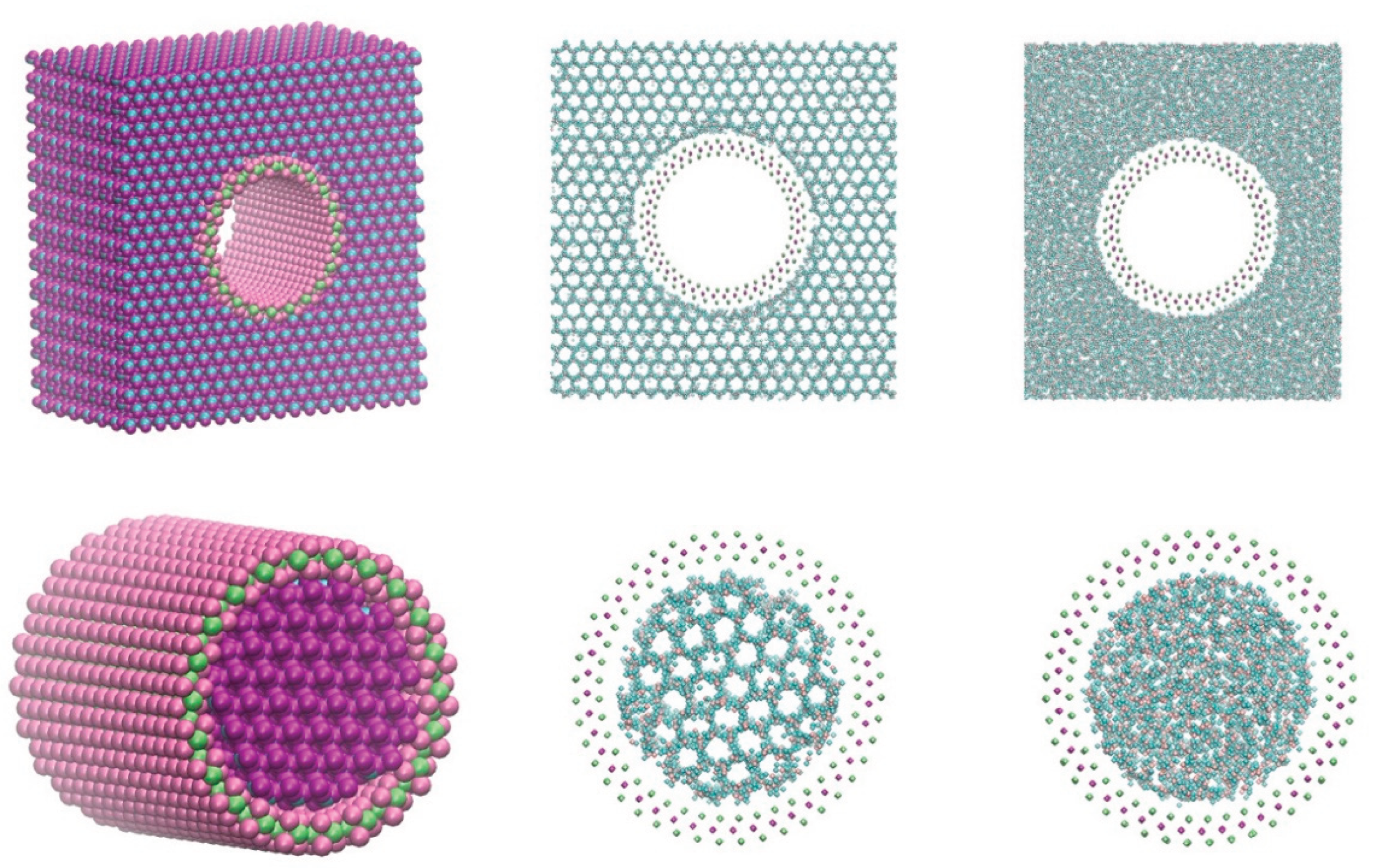
Figure 2.
In section a), the evolution of (MSD) is a function of time for the four states of confined ice structures. The top curve (in purple) represents the time evolution for ordered ice placed inside the nanotube, while green represents disordered ice inside the nanotube. Orange represents the evolution of ordered ice in the interstices outside the nanotube, while blue represents disordered ice in the interstices. Different heating rates are shown in section b. phase change in two systems inside the MoS2 nanotube and surrounded by MoS2 nanotubes for complete and hydrogen-defective hexagonal ice ((22, 22) nanotube). In section c, the system's RDF is visible. Figs. b1 and c1 depict a disordered hexagonal ice confined within a nanotube, b2 and c2 depict an ordered hexagonal ice confined within a nanotube, b3 and c3 illustrate a disordered hexagonal ice surrounding the nanotube, and b4 and c4 illustrate an ordered hexagonal ice surrounds the nanotube. The system's behavior is visible in the bottom snapshots.
Disclaimer/Publisher’s Note: The statements, opinions and data contained in all publications are solely those of the individual author(s) and contributor(s) and not of MDPI and/or the editor(s). MDPI and/or the editor(s) disclaim responsibility for any injury to people or property resulting from any ideas, methods, instructions or products referred to in the content. |
© 2025 by the authors. Licensee MDPI, Basel, Switzerland. This article is an open access article distributed under the terms and conditions of the Creative Commons Attribution (CC BY) license (http://creativecommons.org/licenses/by/4.0/).
Copyright: This open access article is published under a Creative Commons CC BY 4.0 license, which permit the free download, distribution, and reuse, provided that the author and preprint are cited in any reuse.


