
Submitted:
04 June 2025
Posted:
05 June 2025
You are already at the latest version
Abstract
The concept of the static and dynamic reservoirs is presented and their performances are evaluated. The static reservoir is a simple reservoir with constant volume and the dynamic one has a volume which varies in function of the position of an internal piston coupled to a spring. The spring is compressed while the pressure in the chamber rises and exerts a proportional force on it. The two reservoirs are components to be used in compressed air energy storage systems. The study comprises a model of the compression machine as also models of the two reservoirs. The filling processes are simulated and the different variables are represented in function of the time. A reduced scale experimentation set-up is presented and its behaviour is first simulated. Then the results are compared to the experimental records.
Keywords:
Compressed air
; energy storage
; static reservoir
; dynamic reservoir
; modeling of a compressor
; energy of a loaded spring
1. Introduction
In the context of the global warming and climate change alternative energy sources are called upon to replace traditional fossil sources with the aim of significantly reducing greenhouse gas emissions [1]. Renewable energy sources with the examples of wind energy or photovoltaic generators present the character of intermittency and stochastic or unpredictable production and need to be assisted by important energy storage facilities [2,3]. When the possibilities of realizing large pumped hydro storage installations are limited due to geographical and topographical conditions, their energy capacity is in addition a limiting factor when compared to the huge demand of electric power over countries or continents [4]. As a possible solution which goes in the same direction as the decentralized production [5], local and domestic storage equipment are considered where smaller units would assume the function of equalizing the power demand and bridge the fluctuations of the stochastic production or assuming the day-to-night shift of photovoltaic sources. Electrochemical batteries are currently at the top of the list for domestic applications with their high energy density and with a strong trend towards the reduction of acquisition costs. But several questions remain open regarding the quantity of materials available for mass production, the question of recycling techniques, in relation to the limited number of cycles or even the associated aging phenomena.
A possible alternative to the electrochemical batteries is given by the compressed air energy storage CAES which has been studied and proposed for large facilities [6,7,8] and for smaller units [9]. Due to the limited energy capacity of CAES even if the storage pressure is of several hundred of bar, stationary applications have been considered first. But also applications for mobility have been proposed from long time with the example of the Mekarski tramway [10]. More recent realizations for individual mobility and for small range have reached the state of pre-industrialization [11,12].
2. Compressed Air Energy System with Accumulation in a Storage Vessel
A conventional compressed air energy storage system is composed of an air compressor feeding a reservoir in the charging mode and of an expansion machine for the discharging mode. The system is completed by an input and an output interface to the electric system, namely a motor driving the compressor and a generator driven by the expansion turbine (Figure 1). The air reservoir represents the accumulating element of the chain and is the object of the present study.
2.1. Static and Dynamic Reservoirs
Two different systems are evaluated. The first uses a reservoir with constant volume. This system is called the static reservoir and is represented in the Figure 2a. The second system is a reservoir with variable volume as proposed in [14]. The variable volume is obtained by a moving piston inside of the cylindric reservoir and coupled to a spring. The air injected into the reservoir from the compressor moves the piston and compresses the spring where an additional amount of energy is stored. This system is called the dynamic reservoir. A schematic representation is given in Figure 2b. Figure 2c shows the same system in the full state of charge where the space occupied by the spring in its compressed state becomes evident. The two cylindric volumes have the same section. The volume of the dynamic reservoir is equal to the volume of the static reservoir when the position of the piston δ reaches the value of the length l1 of the static reservoir. When the piston is at this position the spring exerts a force equal to the pressure P multiplied by the piston’s surface A.
The pressure P appears in the volume of the cylinder due to the injection of air by the compressor. The pressure is depending on the mass of air inside the volume and its value is given by rel. 2:
where m is the time integral of the massflow imposed by the compressor
2.2. The Model of the Compressor
The compressor is considered as a source of mass in this modelling. Compressors are usually characterized by their nominal volume flowrate . The nominal volume flow rate is expressed in m3 per second from its given value in liter per min. The value of 190l/min is chosen in the considered example and corresponds to the characteristic of the example described in [14].
The real volume flowrate is of a different value due to the effect of the expansion of the dead volume after the end of the discharge when the piston goes in its return stroke. The real volume flowrate is calculated with the help of a so-called volumetric yield defined as
where is the ratio of the top volume to the bottom volume of the compression cylinder.
And the compression ratio or the ratio of the discharge pressure to the suction pressure. It varies from 1 to during a full charging process.
The real volume flowrate becomes
Then, the mass flow rate is calculated as
Numerically, the nominal mass flowrate of the example is calculated
The effect of the expansion of the dead volume is illustrated by the P-V diagram of Figure 3. The piston of the compressor starts to move from the position with the largest volume (Vcyl = Vbott) and the pressure is equal to Psuc (1), (1’). Then when the pressure reaches the discharge value (Pdis, P’dis) (2), (2’) the discharge valve opens and the air is exhausted, the volume decreases down to Vtop = Vd. During the return stroke the suction valve does not open until the pressure of the remaining air in the dead volume decreases under the value of the suction pressure Psuc. The effective suction volume becomes
Vcyl-Vd*Cr,
Leading to the definition of the volumetric yeald
2.3. Modeling the Two Reservoirs
2.3.1. Parameters of the Reservoirs
2.3.2. The Structural Diagram of the Static Reservoir System
Figure 4 gives the structural diagram of the static reservoir system. The real mass flowrate provided by the compressor is accumulated in the reservoir what is represented by the time integral (block 1/s). From the accumulated mass of air the pressure is calculated with an ideal gas law. The actual value of the pressure Pdis is fed back to the calculation of the compression ratio Cr used for the calculation of the volumetric yield.
2.3.3. Structural Diagram of the Dynamic Reservoir System
In the dynamic reservoir system, the pressure exerted on the mobile piston by the injected air produces a displacement of it and a compression of the spring. The system comprises two different energy accumulation elements. First, energy is stored in the form of compressed air in the variable volume of the cylinder and second in the tension of the spring. The calculation of the piston’s position and of the air accumulation volume is realized according to a dynamic model for the association of the mass of the piston and of the spring. The energy accumulated in the form of compressed air is calculated with the same model as for the static piston system described in the previous section, namely via the accumulated mass of air in the chamber and an associated state equation. In this case the accumulation volume varies with the position of the piston.
2.3.4. The Model of the spring-Mass System
The description of the movement of the piston and its impact on the compression of the spring can only be made by using a model based on integral causality [15,16]. So the piston and the storage spring are modelled as a classical damped mechanical oscillator as represented in Figure 5. The spring characteristic and the corresponding differential equation can be written as:
m is the mass of the mobile piston.
The force caused by a thermodynamic effect Ftherm is the difference of the force caused by the pressure in the cylinder’s chamber (absolute value) on the front side of the piston, minus the effect of the atmospheric pressure on the rear side of the piston. K is the spring constant and μ the velocity-dependent friction coefficient.
The structural diagram of the dynamic reservoir system is given in Figure 6. The compressor model is identic to the model used previously and uses the principle of the volumetric yield. The state equation considers the variable volume depending on the piston’s position. The diagram includes the damped mass-spring model.
2.4. Energies Accumulated
2.4.1. Volume of Air
The energy content of the volume of air depends on its volume, pressure and temperature. In the present system where the piston moves slowly the thermodynamic phenomenon can be considered as evolving according to an isothermal characteristic. In the full state of charge, the pressure is of 6bar in a volume of 0.1 m3. The corresponding stored energy is calculated as
This value is in the air volume in both cases, constant volume and variable volume when it reaches its maximum (0.1m3) and when the pressure is identic. The simulation of the charging process presented in the next section will show that this state of the variable volume is reached for t= 340s (Figure 12). It is also the time where the pressure of 6bar is reached. For the constant volume system the pressure of 6bar is reached after a time of 254s.This confirms that the spring model and parameters are right.
2.4.2. Energy Accumulated in the Spring
With
Then
When k=61.7kN/m and x=0.9m
3. Simulation Results
The structural diagrams of the static and dynamic reservoir systems have been implemented in a numeric simulation (Simulink) and produce the evolution of the different variables as functions of the time. In the static reservoir the accumulated mass of air and the pressure in the reservoir are relevant For the dynamic reservoir additional variables as the force exerted on the piston, its displacement and the variable volume are considered.
3.1. Evolution of the Pressures and Masses of Air
The evolution of the pressure in the static and dynamic reservoirs is presented in Figure 7. The blue curve shows the evolution of the pressure in the constant volume system and the red one the pressure in the variable volume with spring.
The evolution of the pressures is the result of the accumulated amount of air in the volumes (Figure 8) due to the injection by the compressor of the corresponding massflows (Figure 9). The blue colour is again associated to the constant volume system and the red to the variable volume. The same masses of air are accumulated at the corresponding instants where the pressures are identical (254s and 340s).
3.2. Evolution of the Mechanical Variables
In opposition to the static reservoir where only the pressure changes, the geometry of the dynamic reservoir evolves according to the change of the pressure. The elevation of the pressure in the variable volume cylinder produces a directly proportional force. The evolution of the force in function of time is represented in Figure 10. From this force the characteristic of the spring produces a displacement of the piston which further increases the active volume of the cylinder. The variation of the position of the piston is also directly proportional to the force as also the variation of the volume. The corresponding curves are given in Figure 11 and Figure 12. On these figures one can see that the values reached at the time where the pressure is equal to 6bar (340s) correspond to the correct design of the system (0.9 m and 0.1m3)
3.3. Evolution of the Energies Stored in the Systems
In the static reservoir energy is only stored in the volume of air. Concerning the dynamic reservoir energy is stored in the volume of compressed air and in addition in the loaded spring. The different values of stored energy are indicated in Figure 13. The content in the static reservoir with constant volume is indicated in blue. The value of 57505 J (rel. 15) is reached at the time t=242s. The same value is reached for the variable volume of the dynamic reservoir at the time t=340s (red curve). The energy stored in the spring reaches the value of 24.9kJ at the same time (black curve). Finaly the total amount of stored energy in the dynamic reservoir (air and spring) is represented by the yellow curve. At the full state of charge the dynamic reservoir has accumulated the value of
This value represents an increase of 43% referred to the static reservoir.
4. Analysis and Experimentation with a Small-Scale System
A small experimentation facility has been realized comprising a compression machine and a fixed volume reservoir. Then the facility is completed with a reduced scale dynamic reservoir. The compression machine is realized on the base of a pneumatic cylinder moved with a crankshaft, itself driven by a geared variable speed electric motor. The compression machine feeds a small reservoir of 0.3dm3 capacity through an anti-return valve. The compression machine together with the small reservoir are represented in Figure 14.
4.1. Numeric Values of the Small Experimental Static Reservoir
The small experimentation set-up is realized with simple components available on the market and which allows to verify the principles of the static and of the dynamic reservoirs in a simple manner. The global set of parameters is a result of using already available components at the author’s facility.
Compression machine
Diameter of the piston : 12 mm
Course du piston : 100 mm
Volumetric ratio (Vtop/Vdown) : 0.12
Reservoir
Volume: 0.3 l
Rotational speed of the drive : 2 revol./sec
The volume of the cylinder of the compressor is calculated (rel. 22)
With the value of the rotational speed the volume flowrate becomes
4.2. The small-Scale Dynamic Reservoir
The reduced scale model of the dynamic reservoir is realized with a classic pneumatic cylinder used as a variable volume. This cylinder is coupled to two parallel running springs outside of the cylinder. This configuration is chosen in dependency of available industrial components. The parameters of the set-up components are listed in Table 2. The realized set-up is shown in Figure 15.
When the volume of the cylinder reaches the same value as of the fixed reservoir (0.3dm3), the piston has moved of xn
The two parallel running springs have the characteristics given in Table 2
For a volume of 0.3l, the force of the spring pair becomes
On the rear side of the piston the atmospheric pressure exerts a counter force of
The pressure in the cylinder must generate a force able to compensate the force of the spring and of the atmosphere.
As indicated in Figure 16 the variable volume of the dynamic reservoir reaches the value of 0.3dm3 at time t=134.7 sec. At that time the pressure in the dynamic reservoir reaches the value of 5.32*105N/m2 (Figure 17). From the same figure one can see that the pressure in the static reservoir reaches the same value earlier at time t=97sec.
4.3. Experimental Results
An experimental verification has recorded the values of the pressure in the reservoirs. They are reported on the same diagram of Figure 17. The pressure in the static reservoir is noted with (X). The pressure in the dynamic reservoir is represented in Figure 17b together with the measured values.
The pressure values indicated in Figure 17 are obtained from the calculation of the accumulated mass of air in the reservoirs. These masses are the result of the time integration of the corresponding massflows provided by the compression machine. The accumulated masses of air are represented in Figure 18 and the corresponding massflows in Figure 19.
Figure 20 shows the evolution of the piston’s position when the variable volume is filled by the compressor. The simulated value of the position reached when the pressure is of 5.32 bar corresponds to the calculated value according to rel. 24. The measured positions from the set-up are also indicated in the figure (x). There is an important difference between the calculated positions and the measured ones. There was also a difference between the measured and calculated pressures (Figure 17b). But the relations between measured pressures and positions correspond to the real values of the system (piston surface and spring constant). This indicates that the differences between simulated and calculated values is due to a not realistic representation of the accumulation process of air in the reservoir. The assumption of an isothermal pressure rise in the reservoir and a not verified value of the dead volume effect can be the main reason for the difference between simulated and measured values. The small dimensions of the experimentation set-up may also have an influence.
To complete the presentation of the simulated variables, the force on the piston is represented in Figure 21.
5. Discussion
The present paper illustrates the behaviour and properties of the so-called dynamic reservoir where a mobile piston and a compression spring are integrated in the reservoir. With an identical accumulation volume as that of a classical constant volume compressed air energy storage system, the new dynamic reservoir presents an increased energy capacity due to an accumulation of mechanical energy in the spring. The calculated benefit of capacity is around 50% (rel. 14 and 19, and as represented in Figure 13. This value should however be compared with the capacity increase when a constant volume reservoir is designed according to the real dimensions and space occupied by the compressed spring. The relation between the lengths of the deployed and compressed spring is supposed to be in a ratio of 3 to 1 (L0 to LN in Figure 2). As a consequence the increased value of the volume adapted to the real dimension occupied by the spring would increase the energy capacity of a static reservoir to nearly the same value as the dynamic reservoir. The augmented static reservoir would have the advantage of a reduced number of components (no spring, no piston no guidance rod and no sealing joints) and would be consequently much cheaper. One advantage of the dynamic reservoir would be to benefit from pressure which is a little higher then the pressure of the static one by a low state of charge.
6. Conclusions
A compressed air energy storage system uses traditionally pressurized reservoir which determines the energy capacity. A new proposal recently made proposes to add inside of a cylindric one a piston compressing a spring to add mechanical storage. This paper has evaluated and simulated and compared the two systems from the point of the storage capacity and the variation of the pressure in dependency of the state of charge. The simulation has included a specific model of a compression stage where the parasitic effects like the expansion of the dead volumes on the mass florate is considered. The limited benefits of the added piston-spring assembly have been discussed in a specific paragraph.
Funding
This research received no external funding.
Conflicts of Interest
The author declares no conflict of interest.
References
- IPCC Intergovernmental Panel on Climate Change (IPCC) Synthesis Report 2024,.
- https://www.ipcc.ch/synthesis-report/.
- Rufer A., Energy storage – Systems and Components,.
- Ruiming Fang, Ronghui Zhang, Advances in Hybrid Energy Storage Systems and Smart Energy Grid Applications, Special issue of the Journal of Energy Storage, Elsevier, 23 September 2021, https://www.sciencedirect.com/special-issue/10GRJ69GC0Q accessed April 4th 2025. [CrossRef]
- World energy outlook 2024 IEA, International Energy Agency.
- https://iea.blob.core.windows.net/assets/a5ba91c9-a41c-420c-b42e-1d3e9b96a215/WorldEnergyOutlook2024.pdf.
- Ali M. Adil a, Yekang Ko, Socio-technical evolution of Decentralized Energy Systems: A critical review and implications for urban planning and policy, Renewable and Sustainable Energy Reviews 57 (2016) 1025–1037, Elsevier.
- Lehmann, J., Air storage gas turbine power plants, a major distribution for energy storage, International Conference on Energy Storage, Brighton, U.K., April 1981, pp.327–336.
- The Mc Intosh CAES Power Plant, http://www.powersouth.com/files/CAES%20 Brochure%20[FINAL].pdf. Accessed on September 22, 2017.
- Bradshaw, D. T., Pumped hydroelectric storage (PHS) and compressed air energy storage.
- (CAES), Power Engineering Society Summer Meeting, Seattle, WA, July 16–20, 2000, Vol. 3, pp. 1551–1573.
- Kermit, A., CAES: The underground portion, IEEE Transactions on Power Apparatus and Systems, PAS-104(4), 809–812, 1985. [CrossRef]
- Electricity storage. Heat. Cold. Compressed air. Combined in a sustainable system, https://www.green-y.ch/en/.
- Radeska, T ., The Mekarski system—Compressed-air propulsion system for trams, The Vintage News, October 17, 2016 [online], https://www.thevintagenews.com/2016/10/17/the-mekarski-system-compressed-air-propulsionsystem for-trams/. Accessed on July 28, 2017.
- L. Blain, “AIRPod: tiny air-powered commuter costs half a Euro per 100km.,” 2009. [Online]. Available:https://newatlas.com/airpod-compressed-air-car-mdi-zeroemissions/11177/ or https://www.mdi.lu/airpod2. [Accessed 27 April 2018].
- MDI.lu,” Motor Development International, 2018. [Online]. Available: https://www.mdi.lu. [Accessed 05 May 2019].
- Kabinga R.K.N., Tartibu L.K., Okwu M.O., Development and performance evaluation of a dynamic compressed air energy storage system, IMECE 2020, International Mechanical Engineering Congress and Expo, November 16-19, 2020, Portland USA, Proceedings of the ASME 2020.
- Yuan Cheng; Keyu Chen; C.C. Chan; Alain Bouscayrol; Shumei Cui, Global modeling and control strategy simulation, IEEE Vehicular Technology Magazine ( Volume: 4, Issue: 2, June 2009). [CrossRef]
- Michael Shaerer, Pierre Gremaud, Periodic motion of a mass–spring system, IMA Journal of Applied Mathematics ( Volume: 74, Issue: 6, December 2009).
Figure 1.
Compressed air energy storage system.
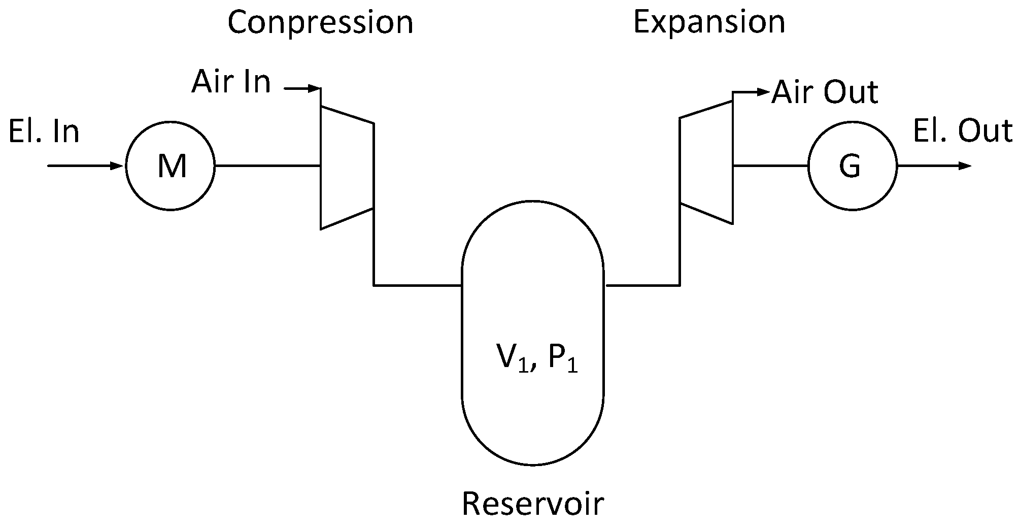
Figure 2.
Static a) and dynamic b) compressed air reservoirs. c) dynamic res. full loaded.
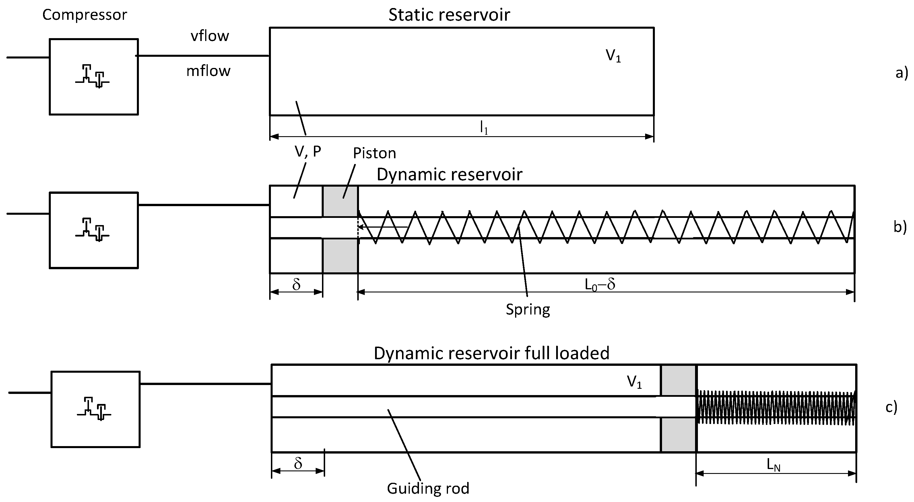
Figure 3.
Effect of the expansion of the dead volume.
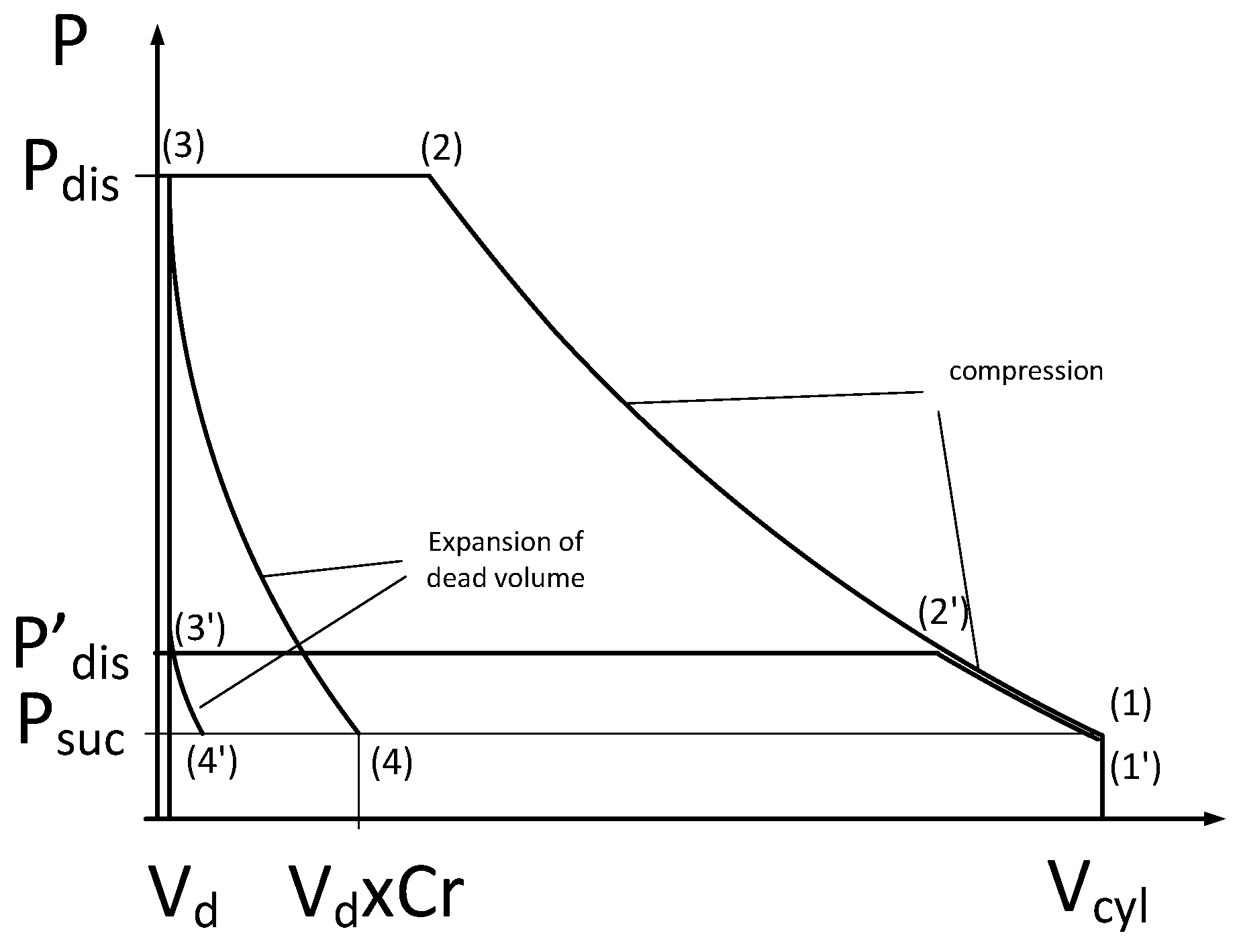
Figure 4.
Structural diagram of the static reservoir system.
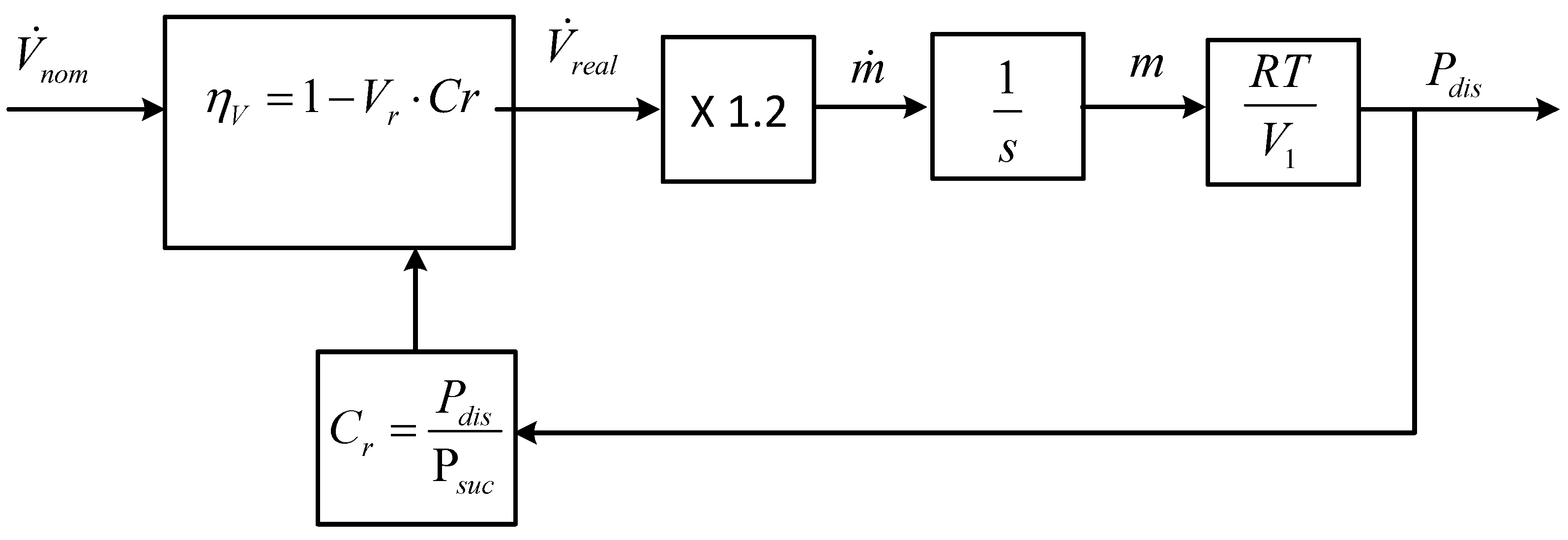
Figure 5.
Schematic representation of the mass-spring system.
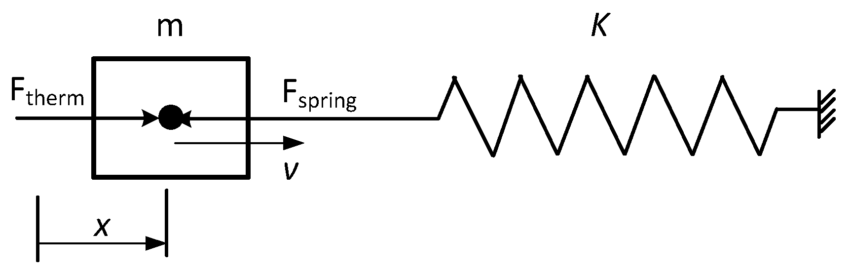
Figure 6.
Structural diagram of the dynamic reservoir system.
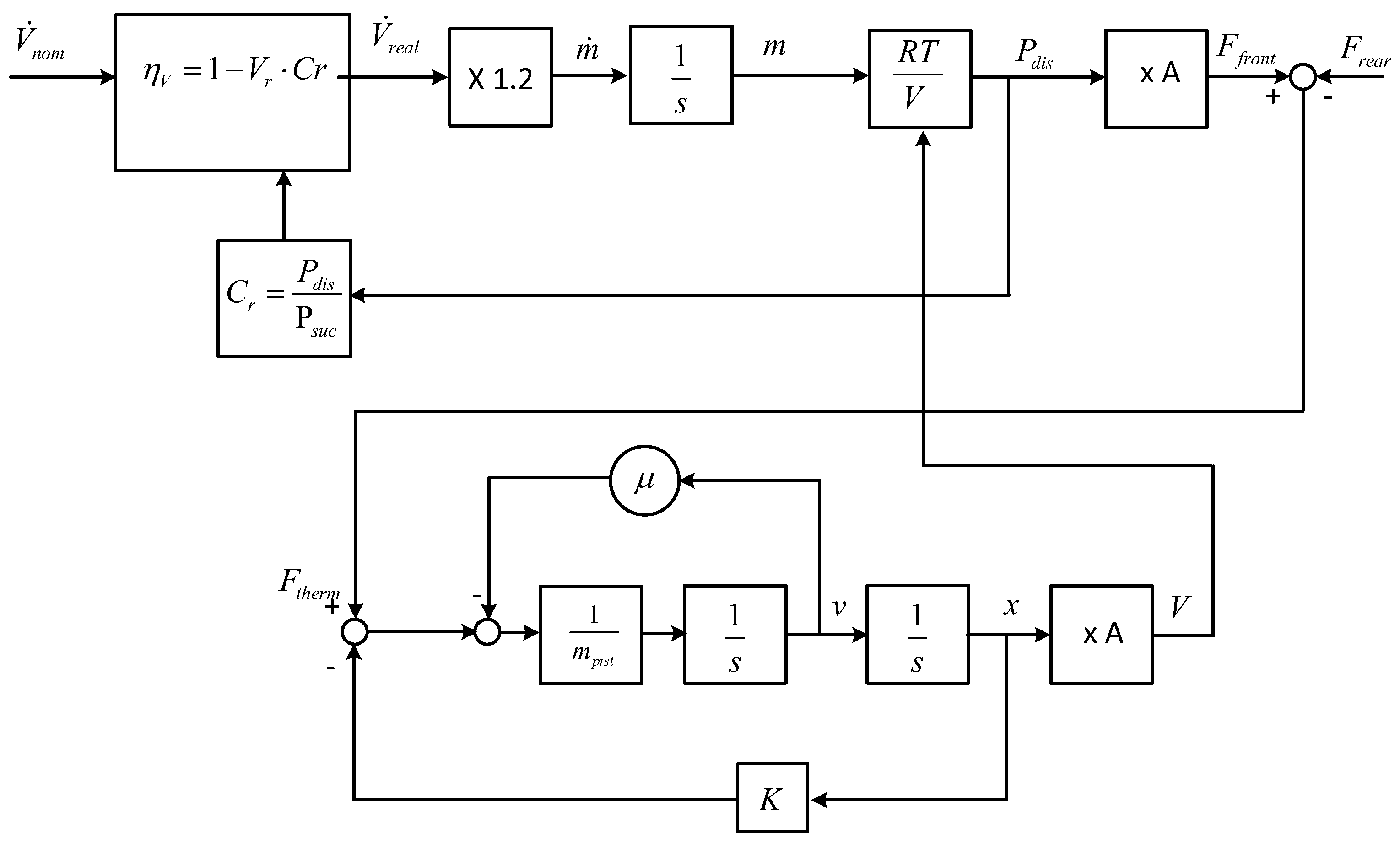
Figure 7.
Pressure in the reservoirs (constant volume : blue, variable volume : red).
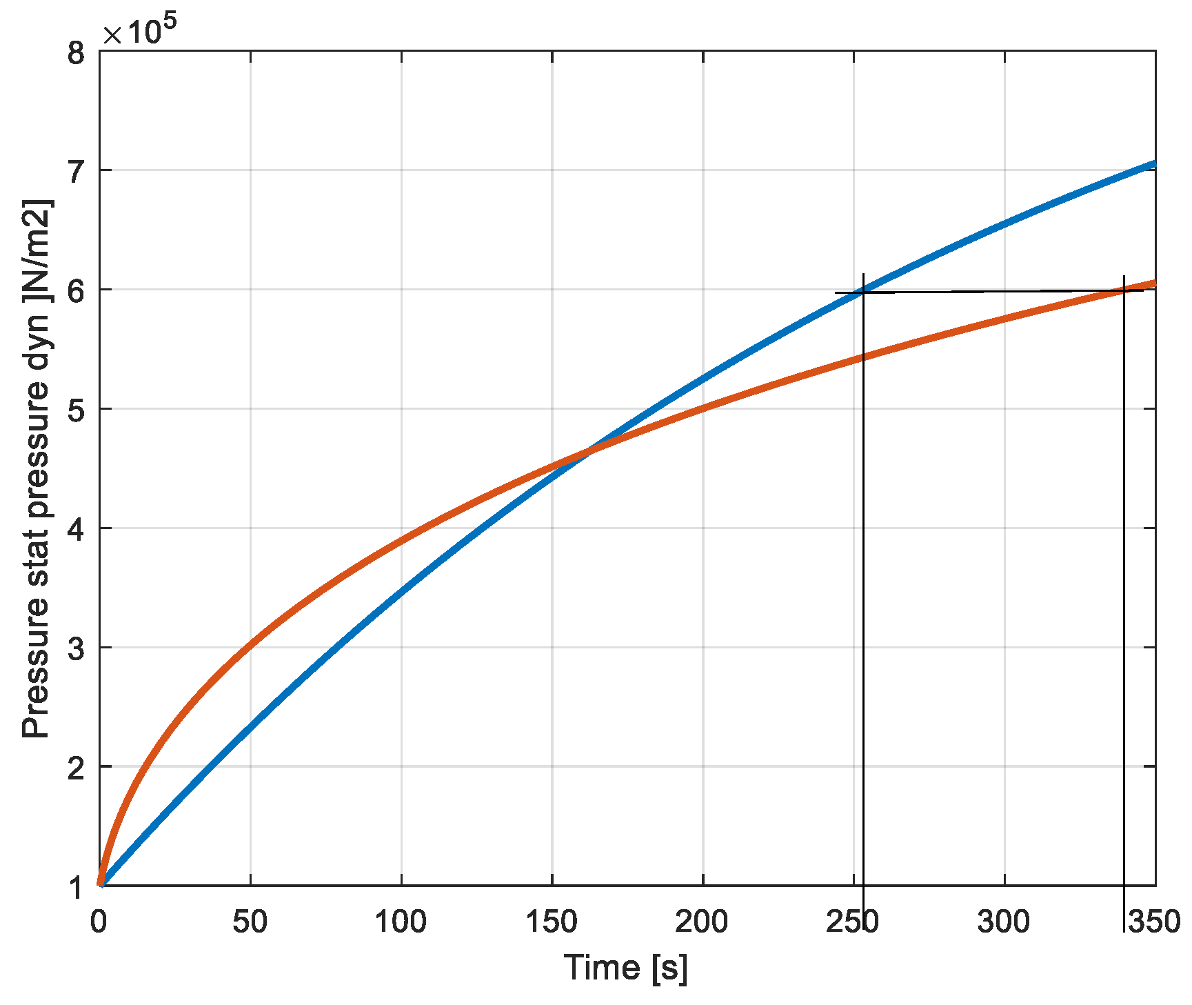
Figure 8.
Mass of air accumulated in the two reservoirs (blue: constant volume, red: variable volume.
Figure 8.
Mass of air accumulated in the two reservoirs (blue: constant volume, red: variable volume.
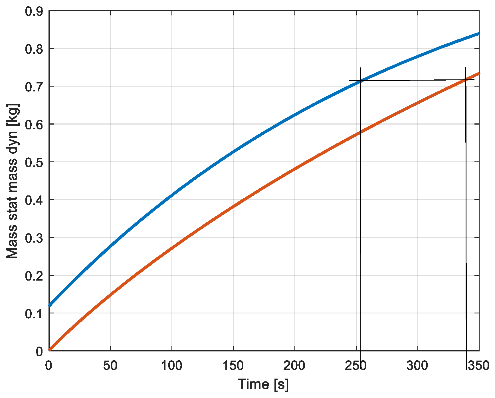
Figure 9.
Massflows to the reservoirs (blue: constant volume red: variable volume).
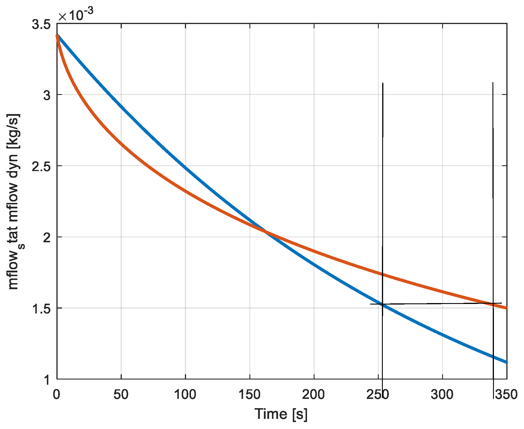
Figure 10.
Evolution of the force in function of time.
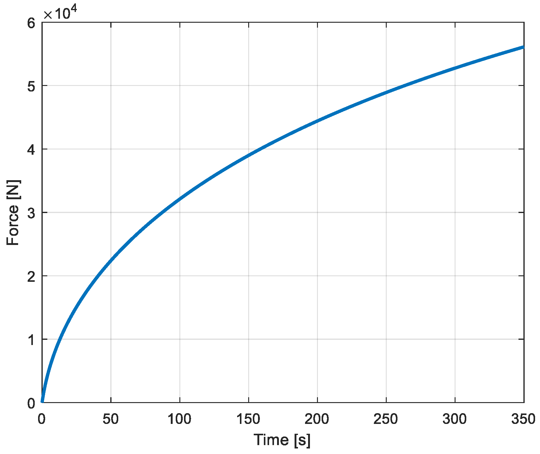
Figure 11.
Position of the piston.
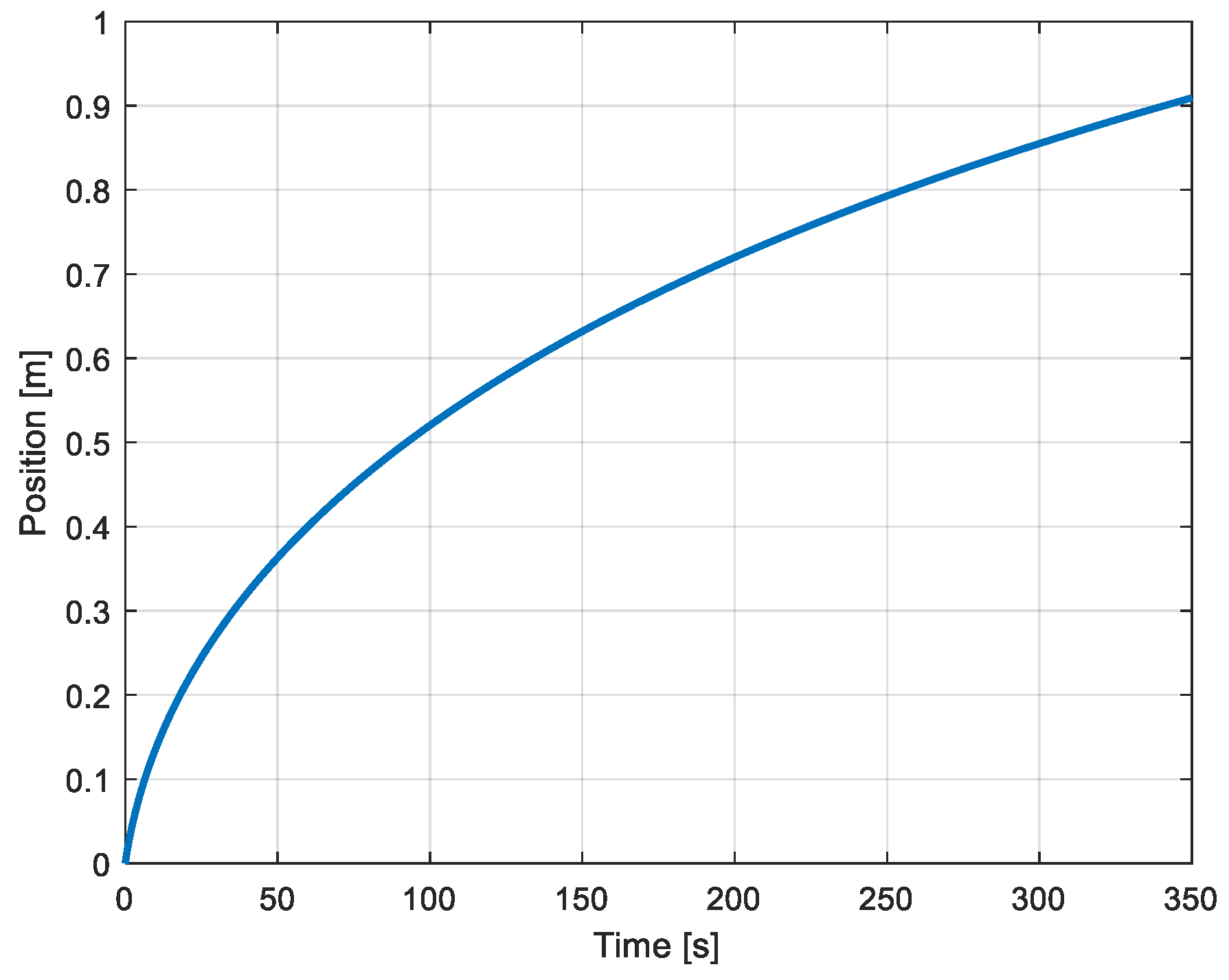
Figure 12.
Volume of the dynamic reservoir.
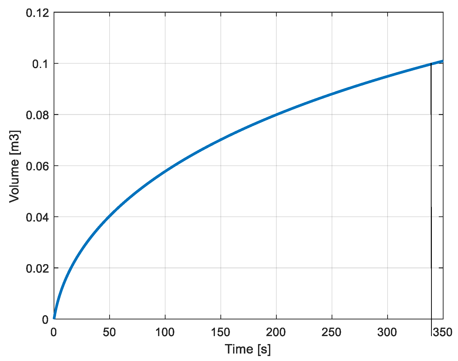
Figure 13.
Energies accumulated in the static and dynamic reservoirs. Compressed air energy in the fixed reservoir (blue curve); compressed air energy in the variable volume (red curve); Energy accumulated in the spring (black curve); total energy of the dynamic reservoir (yellow curve).
Figure 13.
Energies accumulated in the static and dynamic reservoirs. Compressed air energy in the fixed reservoir (blue curve); compressed air energy in the variable volume (red curve); Energy accumulated in the spring (black curve); total energy of the dynamic reservoir (yellow curve).
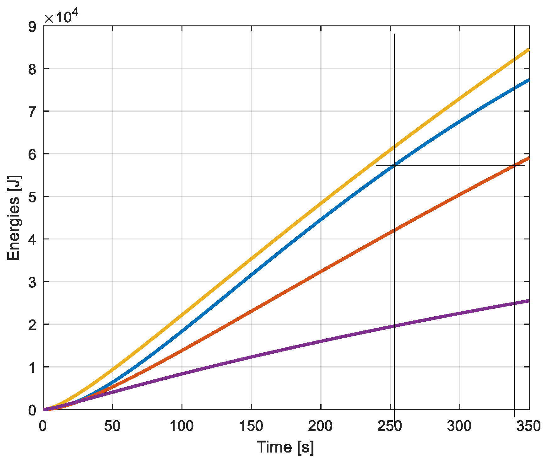
Figure 14.
Small scale of the compression machine and of the fixed volume reservoir.
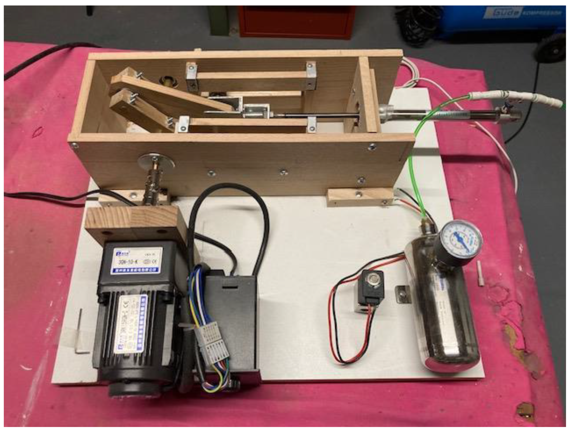
Figure 15.
Reduced scale set-up of the dynamic reservoir. a): unloaded system, b): system loaded at nominal pressure.
Figure 15.
Reduced scale set-up of the dynamic reservoir. a): unloaded system, b): system loaded at nominal pressure.
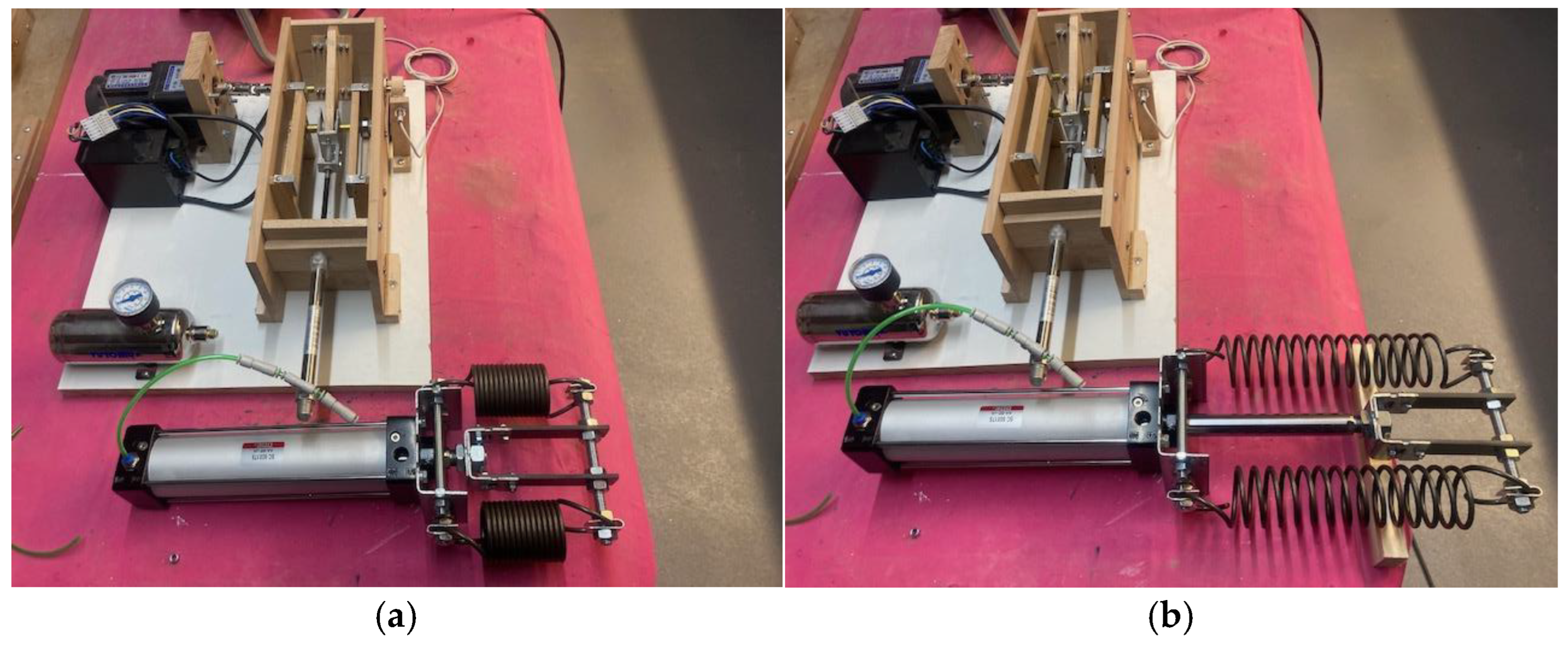
Figure 16.
Volumes of the static (blue curve) and of the dynamic reservoir (red curve).
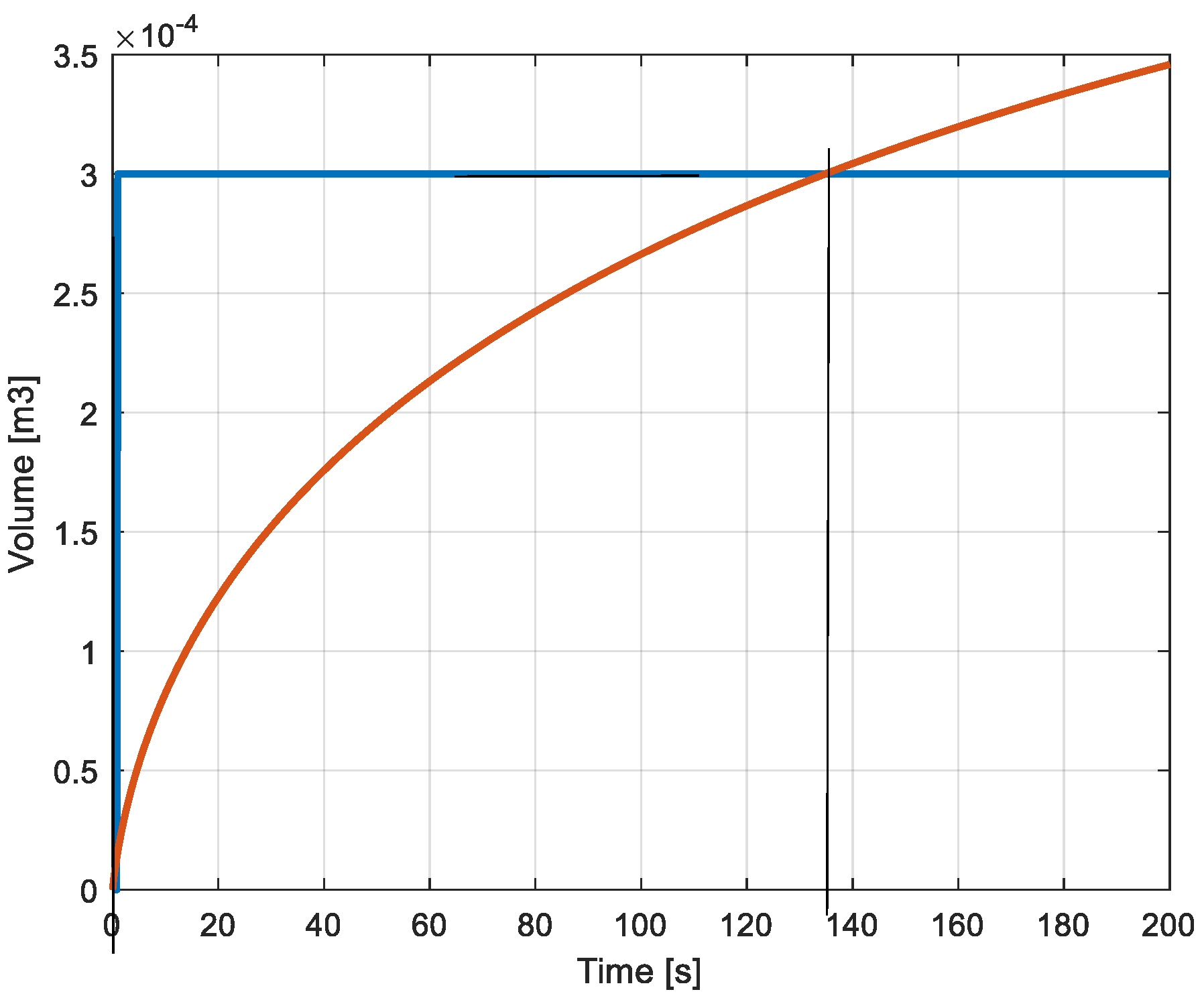
Figure 17.
(a) Pressures in the static (blue) and dynamic reservoir (red). (b) Pressure in the dynamic reservoir -: calculated, x: measured.
Figure 17.
(a) Pressures in the static (blue) and dynamic reservoir (red). (b) Pressure in the dynamic reservoir -: calculated, x: measured.
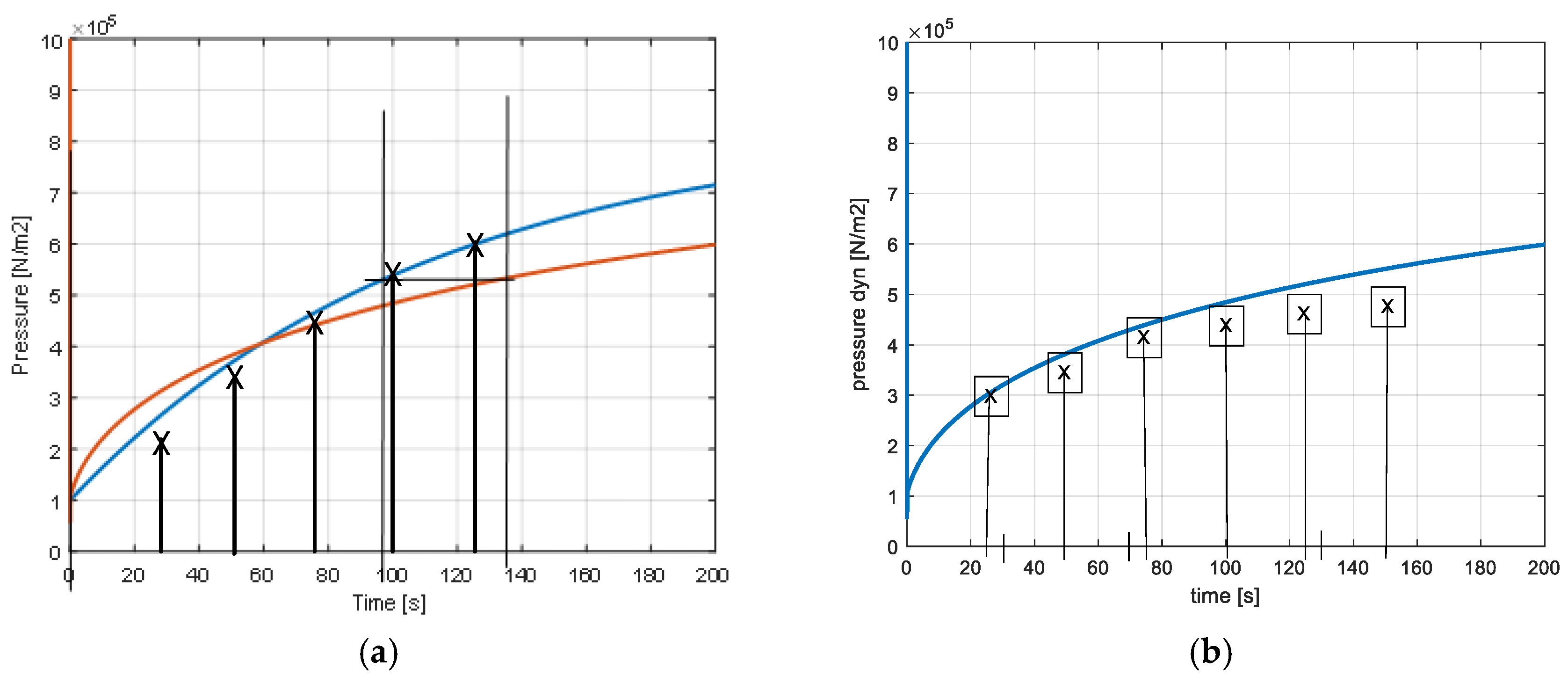
Figure 18.
Masses accumulated in the reservoirs (blue: static res.; red: dynamic res.).
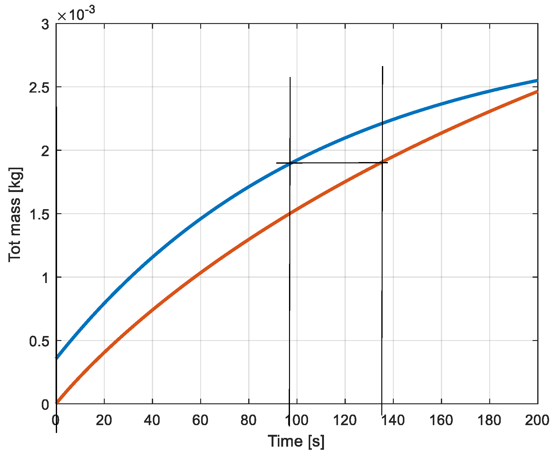
Figure 19.
Massflows provided by the compression machine (blue: static reservoir, red: dynamic reservoir.
Figure 19.
Massflows provided by the compression machine (blue: static reservoir, red: dynamic reservoir.
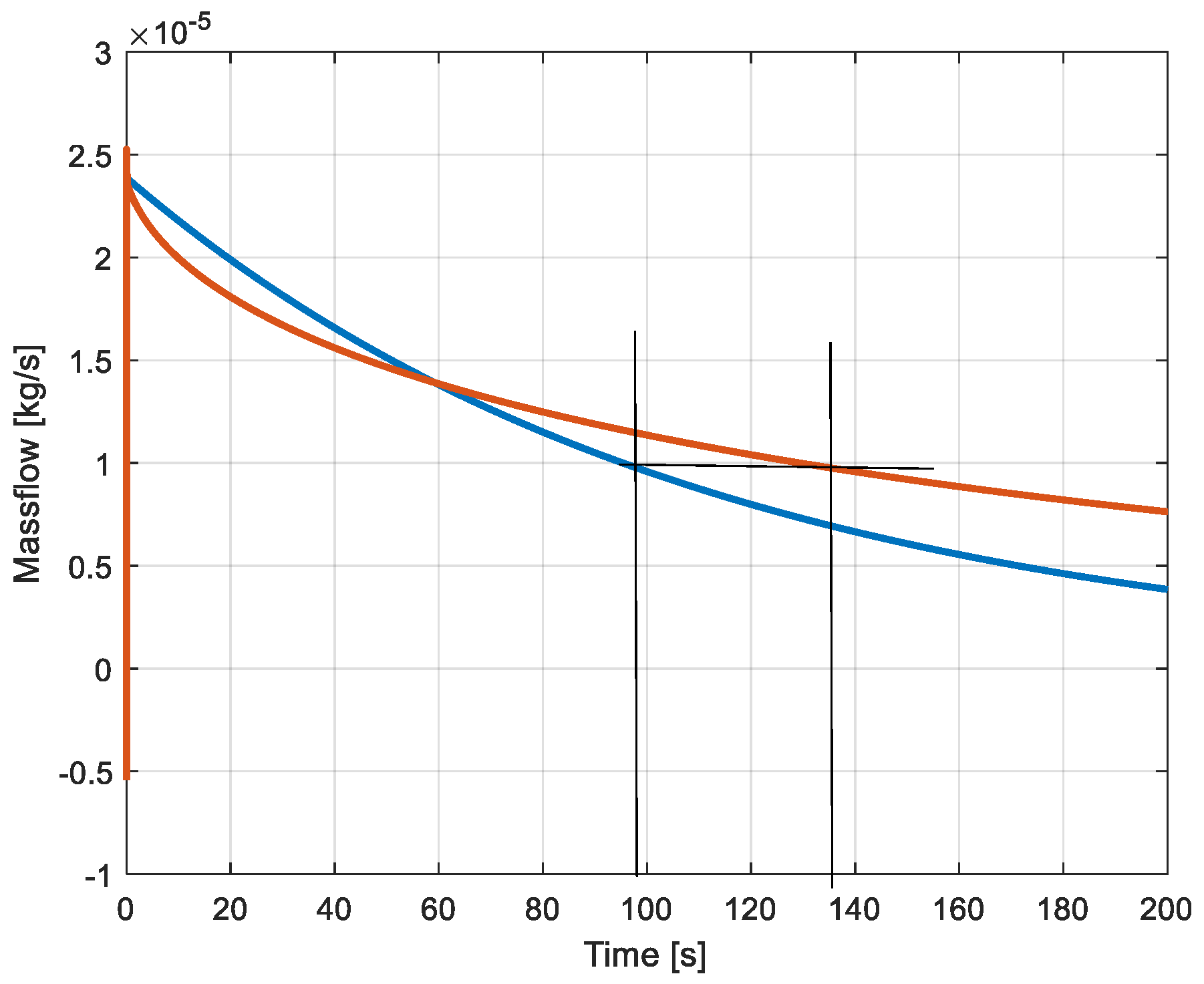
Figure 20.
Position of the piston (dynamic reservoir).
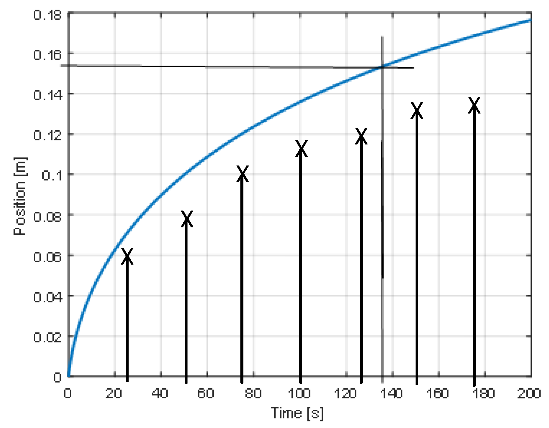
Figure 21.
Force exerted on the piston.
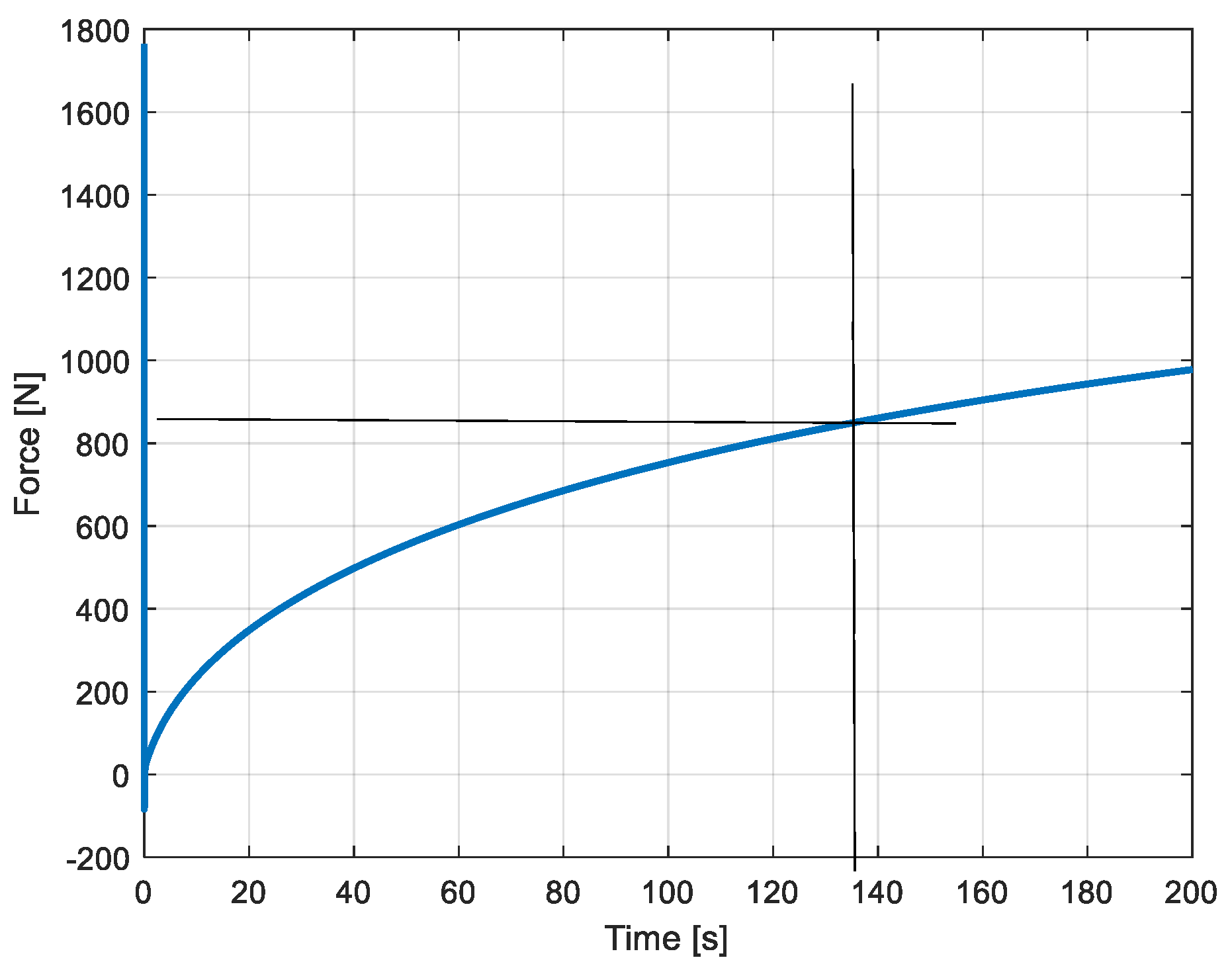

Table 1.
Parameters of the static and dynamic reservoirs.
| Static reservoir | |
| Volume | 0.1m3 |
| Dynamic reservoir | |
| Variable volume | 0 – 0.1m3 |
| Stroke of the piston | 0.9m |
| Surface of the piston | 0.111m2 |
| Constant of the spring | 61.7kN/m |
| Moving mass | 10kg |
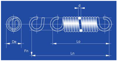
Table 2.
Parameters of the cylinder and of the spring.
| Pneumatic cylinder | SC50X175 |
| Diameter of the piston | 50mm |
| Area of the piston | 0.00196m2 |
| Maximal stroke | 175mm |
| Spring | T33220 |
| De (external diameter) | 50mm |
| D (diameter of the string) | 4.5mm |
| L0 (initial length) | 142mm |
| Ln (length under nominal load) | 280mm |
| Fn (nominal load) | 451N |
| C (spring constant) | 2.77 *103N/m |
| De (external diameter) | 50mm |
 | |
Disclaimer/Publisher’s Note: The statements, opinions and data contained in all publications are solely those of the individual author(s) and contributor(s) and not of MDPI and/or the editor(s). MDPI and/or the editor(s) disclaim responsibility for any injury to people or property resulting from any ideas, methods, instructions or products referred to in the content. |
© 2025 by the authors. Licensee MDPI, Basel, Switzerland. This article is an open access article distributed under the terms and conditions of the Creative Commons Attribution (CC BY) license (http://creativecommons.org/licenses/by/4.0/).
Copyright: This open access article is published under a Creative Commons CC BY 4.0 license, which permit the free download, distribution, and reuse, provided that the author and preprint are cited in any reuse.


