
Submitted:
04 June 2025
Posted:
04 June 2025
You are already at the latest version
Abstract
The Jarzynski’s equality, a remarkable result in modern statistical mechanics, allows us to calculate the free energy of a system, which is a function of state defined only for equilibrium states, from an exponential average of work values resulting from a large number of realizations of a process in which the system goes through, and ends at, out-of-equilibrium states. Limitations to the applicability of this equality are mainly due to the dearth of work values corresponding to infrequent, but dominant, realizations known as rare events. Adopting a heuristic approach, we present a simple example to illustrate the relevance of rare events by analyzing the numerical results of a single-particle stochastic thermodynamic model. We discuss how the applicability of the Jarzynski’s equality depends on the number and distribution of rare events, which in turn are determined by the number of repetitions of a work process and its duration, as well as on the rate at which work is performed on the system. Data explorations similar to the one carried out here can be used to asses if free energies calculated from experimental data or more realistic models are reproducible, typical or random results.
Keywords:
rare events
; Jarzynski’s equality
; stochastic thermodynamics
; out-of-equilibrium processes
1. Introduction
The second law of thermodynamics states that if an amount of work W is performed on a macroscopic system, initially in thermodynamic equilibrium, the following relation is satisfied [1]:
where ΔF is the corresponding increment of the system’s free energy. W – ΔF can be identified as the energy that is dissipated as heat. If no heat is dissipated, we say that work is done reversibly. This occurs when the system and its environment remain in thermodynamic equilibrium during the whole process. Typically, when performing work at a finite rate we have that W > ΔF.
As has been demonstrated experimentally in the last few decades [2,3,4,5,6], Relation (1) is not necessarily obeyed when work is performed on a microscopic or mesoscopic system. (Following Reference 7, we define a mesoscopic system as “… a physical system characterized by energy differences among its states on the order of the thermal energy kBT …” T stands for temperature and kB for Boltzmann’s constant.) In this paper we will use the term small system to refer to either a mesoscopic or a microscopic system. The work performed on a small system displays a fluctuating nature. Multiple repetitions of the same work process will produce a relatively broad distribution of W, which typically would include values smaller and larger than ΔF. (This might lead us to claim that the second law of thermodynamics is broken occasionally at the small scale; however, we can take the position that this is not so, by arguing that the second law was originally established for macroscopic system, for which fluctuations can be ignored.)
Consider a small system, in contact with a thermal reservoir at temperature T, that at time t = 0 is in an equilibrium state i, characterized by an initial free energy Fi. Work is performed on the system by varying an externally controlled work parameter λ from an initial value λi to λf. λ can be a degree of freedom, the system volume, etc. [6,8,9]; in the model presented in Section 3 work will be done by an electric field that acts on a charged particle. If the process is repeated N times the work performed on the system will vary from repetition to repetition, since at the small scale thermal noise is relevant and the system energy has a fluctuating nature [6,7,10,11]. Let us denote these work values by W1, W2, …,WN. Typically, the average of W obeys
In this paper we make use of a curly line on top of a symbol, as in , to indicate that such symbol represents a value that has been calculated using a finite set of data. Since in most work processes of interest here the system is driven out of equilibrium, at the end of such processes the system will be in a non-equilibrium state. Ff is the free energy of the system achieved at the completion of a relaxation process that begins at the moment the work parameter has reached its final value λ = λf.
It is important to emphasize that while the initial and final free energies Fi and Ff are functions of state [1], thus defined only for equilibrium states, the work values in Equation (2) correspond, in the cases we are interested in, to processes in which the system is driven out of equilibrium.
The experimental and theoretical determination of ∆F is of fundamental importance in fields such as phase transitions and chemical reactions. One method that has been developed to determine ∆F for processes in which a system is driven through close-to-equilibrium states is thermodynamic integration [11,12]; another is Zwanzig’s perturbation formula, which follows a different approach [11,13]. The challenge has been greater for far-from-equilibrium processes [11]. Thus the relevance of Jarzynski’s nonequilibrium work theorem, a theoretical breakthrough in modern statistical mechanics. In 1997 Jarzynski demonstrated theoretically [6,7,8,9,11] that a relation exists between W and ΔF:
where β = 1/(kBT). Equation (3) is known as the Jarzynski equality (JE). The brackets represent an ensemble average over all possible paths in phase space of the processes with a work parameter varying from λi to λf [9]. Unlike the average work of Relation (2), here we are dealing with averages over infinite number of trials or repetitions and we will call them infinite ensembles. The JE applies to systems of any size. Furthermore, it is valid for any work rate: remarkably, it applies to processes that drive a system through far-from-equilibrium states. However, for macroscopic systems it is practically impossible (experimentally or computationally) to obtain a collection of work distributions complying with the JE. As we will illustrate, this would require that at least a fraction of the repetitions violate Equation (1), which in most cases would constitute extremely unlikely events. On the other hand, for certain small systems, where system energy and work show a fluctuating nature, the JE has been corroborated experimentally. Liphardt and co-workers did just that by mechanically stretching a single RNA molecule reversibly and irreversibly between two conformations; Hummer and Szabo employed the JE to obtain equilibrium free energy profiles from single-molecule non-equilibrium force measurements using a laser tweezer and an atomic force microscope. Computationally the JE has been demonstrated with simple, small systems [14,15].
It is difficult to overemphasize a noteworthy feature of Equation (3): it allows us to quantify an increment or decrement of the free energy F, which is only defined at equilibrium, from work values derived from processes that might drive a system far from equilibrium.
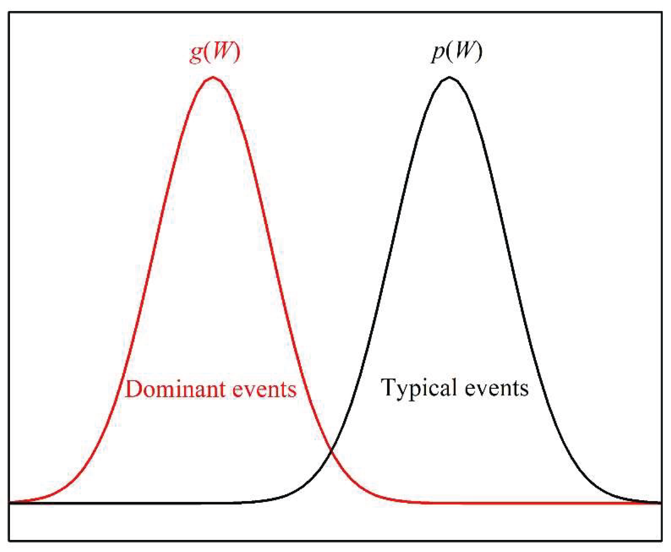
Let us consider the infinite ensemble of all possible processes where work is done on a system by varying a parameter λ from λi to λf. If p(W) represents the corresponding normalized distribution of W, following Reference 16 we can express Equation (3) as
where Wmax and Wmin are the maximum and minimum work performed on the system, respectively, and g(W) = p(W)exp(–βW). Whereas the ensemble average of W, given by is mostly determined by values of p(W) in the proximity of <W> (region of typical events in Figure 1), the ensemble average of the exponential expression g(W) is mostly determined by values at the left tail of p(W) (region of dominant events in Figure 1). For work processes that drive a system out of equilibrium, the events corresponding to the dominant region represent a very small fraction of the total number of events and thus are known as rare events [11,16].
In Reference 16 Jarzynski pointed out that, since the exponential integral in Equation (4) is dominated by rare events, it very often converges poorly. This cannot be ignored when considering practical applications of the JE, because our ability to obtain a good numerical approximation to ΔF depends on the feasibility of performing a large number of experiments or numerical simulations in order to have a large number of rare (dominant) events to achieve a statistically sound evaluation of the integral in Equation (4). To better understand how these experimental or computational limitations affect the applicability of the JE, a single-particle stochastic thermodynamic model is introduced to illustrate, by means of simple numerical calculations, how diverse factors, for example number of repetitions N, work rate, and work process duration, determine the applicability of the JE. In doing so, we discuss concepts relevant to the modern theories of out-of-equilibrium processes, such as system trajectories.
Figure 1.
Schematic representation of the distribution functions p(W) and g(W) = p(W)exp(–βW).
2. Free Energy Calculations from Finite Sets of Data
Since Equation (3) is a theoretical limit that formally applies to an infinite ensemble of work processes, in this section we introduce the formulae used in this paper to discuss the application of the JE to work distributions derived from a finite number of events.
Consider a set of N repetitions of a process in which work is performed on small system, initially in an equilibrium state, by varying a work parameter λ from λi to λf. Let n(Wl) be the number of experiments, or numerical simulations, in which the work done on the system is Wl. Thus,
will be the fraction of experiments or simulations that result in Wl being the work performed on the system. The larger N is, the better will approximate the theoretical limit p in Equation (4):
Likewise, we can define a finite-set case approximation for the exponential expression g(W) in Equation (4):
which in turn has the limit
The average work for this finite-set of experiments or simulations will be given by
We can also establish a finite-set JE relation [see Eq. (3)]:
where lmin and lmax are the subscripts corresponding to the minimum and maximum values of the work done on the system, respectively. is a finite-set approximation to ΔF. In the limit of an infinite number of repetitions we have:
We will show with concrete numerical examples that the difference between and ΔF will depend, among other factors, on the number of repetitions used in Eq. (10) and on the rate at which work is done.
3. Stochastic Thermodynamic Model
Our model consists of a driven Brownian particle p with a positive electric charge q that is immersed in a fluid comprised of charge-less, much smaller molecules or atoms (see Figure 2). Work is done on p by a constant electric field E pointing to the right along the x-axis. Particle p and fluid are in contact with a thermal bath at temperature T. Time t and distance x are discretized quantities. p moves in one dimension along an x-axis and its distance to the origin is given by x=iΔx, where Δx is the length unit and i is an integer number. p is subjected to two forces: a random Brownian force, η, produced by the incessant and chaotic collisions with the molecules or atoms of the fluid (in Figure 1, the red arrow represents the resultant of these random forces), and a second force, fe = qE, produced by the electric field of constant magnitude E, parallel to the x-axis and pointing to the right. (Though Figure 2 is two-dimensional, we only consider the projection of motion of p along the x-axis.)
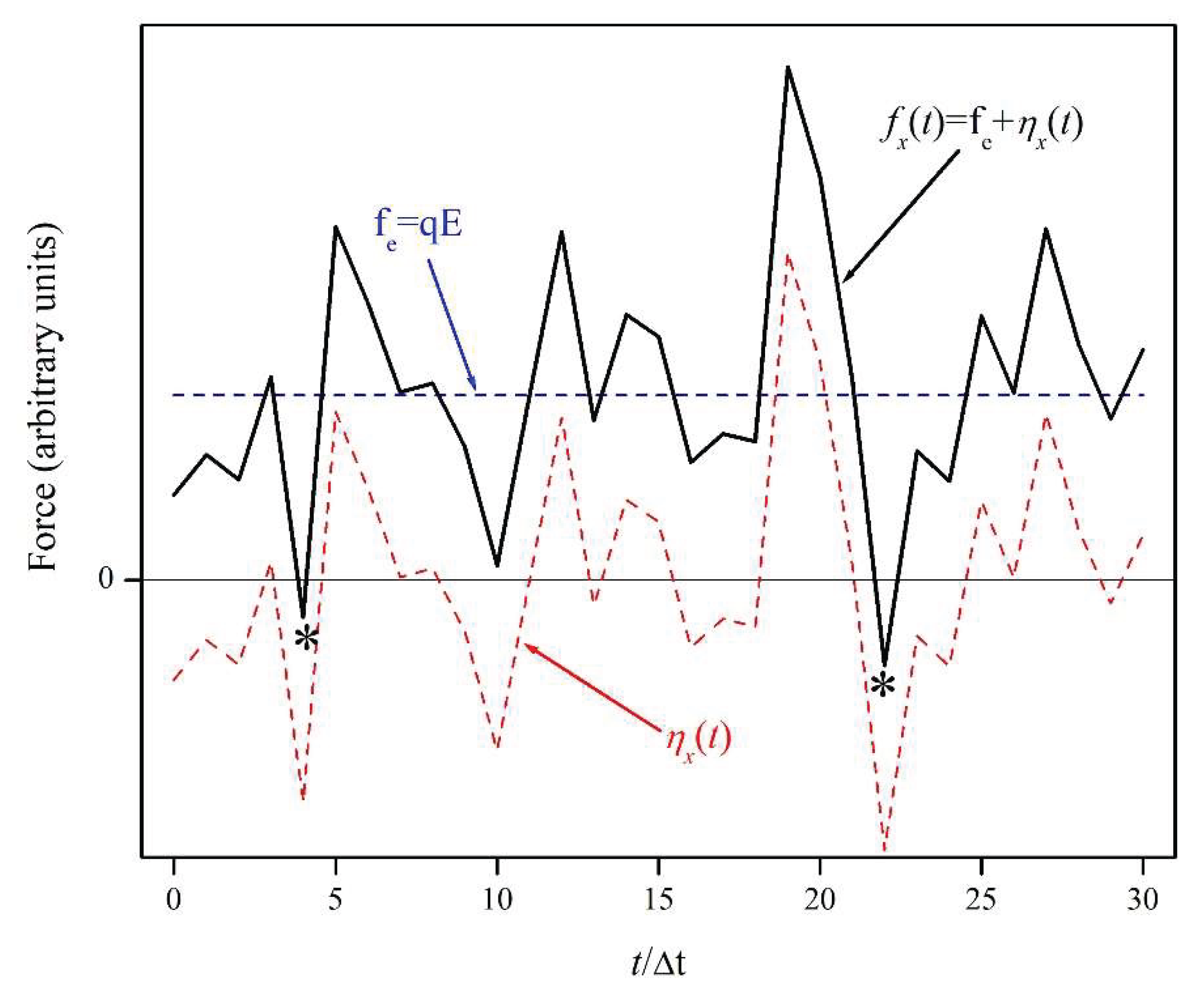
For illustrative purposes, in Figure 3 we plot a possible scenario for the evolution of the forces. The red dashed curve indicates the x-component of η as a function of time, ηx(t), while the blue dashed straight line corresponds to constant electric force; the solid black line represents the x-component of the net force fx(t) = fe + ηx(t). For long times t’, it is expected that the time averages of ηx(t) and fx(t) would be given by
and
Thus, there will be a tendency for p to move to the right. However, due to the random interactions between p and the much smaller particles comprising the fluid, at any time there is a possibility that the net force fx(t) be negative (pointing left), as indicated by the two asterisks.
Figure 2.
A stochastic thermodynamic model consisting of an electrically charged Brownian particle p surrounded by atoms or molecules. An electric field E acts upon p, producing the electric force fe. The collosions between p and the other, much smaller, particles result in the random force η.
Figure 2.
A stochastic thermodynamic model consisting of an electrically charged Brownian particle p surrounded by atoms or molecules. An electric field E acts upon p, producing the electric force fe. The collosions between p and the other, much smaller, particles result in the random force η.
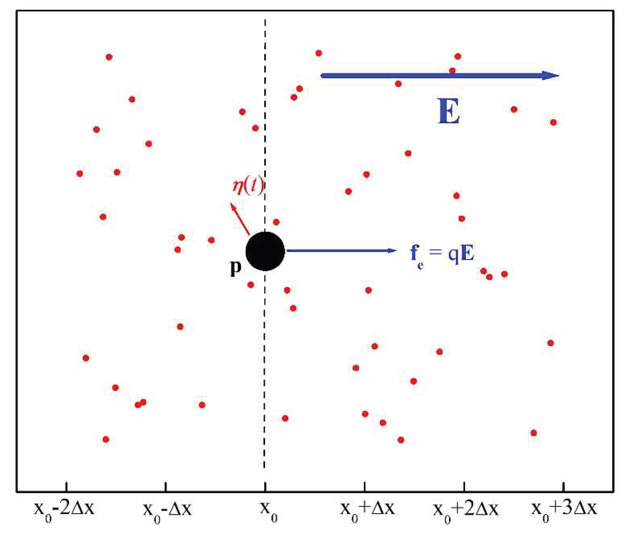
Figure 3.
The x-axis component of the net force acting upon particle p has two components: fe, due to the electric field, and ηx, due to the thermal noise.
Figure 3.
The x-axis component of the net force acting upon particle p has two components: fe, due to the electric field, and ηx, due to the thermal noise.
We assume that particle p is initially at the origin: x(t = 0) = 0. Every time unit Δt, p’s position x is updated: it can move one length unit Δx to the left or to the right, or stay put. Since the work done by the electric force qE on the particle as it moves from site x0 to site (x0 ± ∆x) is ±qE∆x, we adopt the following probabilistic, Markovian rule of motion: If p is located at site xo at time t0, then at time t0 + ∆t, it can remain at x0, with probability
or it can move left to xo – ∆x, with probability
or it can move right to xo + ∆x, with probability
where Z = 1 + exp(+ε/2) + exp(-ε/2), and
ε is a dimensionless energy unit, proportional to the electric field strength, and gives us the electric potential energy difference between two adjacent sites in kBT (= 1/β) units. We also have that P0 + P+ + P– = 1.
Though particle displacements are possible in both directions, the above motion rules introduce a tendency for p to move to right for a non-vanishing electric field.
From Equations (15) and (16) we have that
We will see in the Appendix that this probability ratio can be viewed as a consequence of the fluctuation theorem. This lends theoretical support to our choice of motion rules.
4. Trajectories and Work Distributions
In this section we calculate the work done by the electric field on particle p of the model presented in the previous section. Every realization of this process will give us the position of p as a function of time, what will be termed a trajectory. In contrast to the well-defined thermodynamic properties of a macroscopic system, the microscopic trajectories of p vary from simulation to simulation and manifest a fluctuating, random nature. We will show that the work distributions resulting from large number of simulations often result in smooth curves. By applying the formulae presented in Section 2 to the work distributions obtained with our stochastic model, in Section 5 we calculate .
Suppose that particle p, initially at the origin, is subjected to the random force η(t) and the electric force qE. After τ time units, p will occupy, according to the probabilistic rules of motion of the previous section, a position x(t = τ∆t) = l∆x, where l can take any of the values: -τ, -τ + 1, …, -1, 0, +1, …, +τ. The work done by the electric field will be
We can consider l as a dimensionless distance to the origin and τ a dimensionless time.
Figure 4 shows 20 trajectories of p obtained by running our model with ε = 1 for 20 time units (τ = 20). Recall that ε is proportional to the magnitude of the electric field E (see Equation (17)). The fluctuating nature of the trajectories is expected here because the thermal and electric forces are of comparable magnitude, since for ε = 1 the electric potential difference between two adjacent sites, qEΔx, is equal to kBT. Though in this figure it is difficult to follow individual trajectories, these 20 repetitions clearly show that there is a tendency for p to move in the positive direction. However, in order to obtain distributions from where we can calculate a statistically meaningful free energy, below we resort to much larger number of repetitions N.
Let n(l) = n(Wl) be the number of instances in which the particle ended up, after τ time units, at position x = lΔx, or, what is the same, when the work done by the electric field on p is Wl = εl(kBT) (see Equations (17) and (19)). Illustrating the effect of the electric field strength on p trajectories, Figure 5 shows plots of l versus n(l) for various ε’s, when τ = 20 and N = 106 repetitions. The left-most curve (in black) corresponds to ε = 0 (no electric field). In such case, what we observe is a symmetric Gaussian distribution, as it would be expected for the classical Brownian motion [17]. For the non-vanishing E cases ε = 0.5, 1, and 2, the Gaussian-like distributions are shifted to the right, as p is now more likely to move to the right than to the left. The red curve represents the distribution obtained under the same conditions as in Figure 4 (ε = 1). The most asymmetric distribution (in dark blue) corresponds to ε = 5.
Figure 4.
20 trajectories of p obtained by running our model with ε = qEΔx1 and τ = 20.
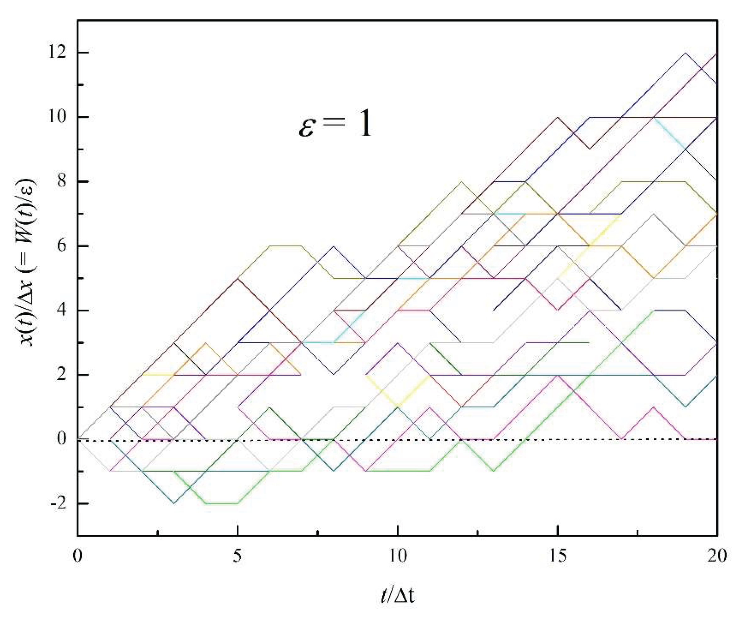
Figure 5.
l vs. n(l) for t = 20Δt and N = 106, for various electric field strengths. ε = βqEΔx.
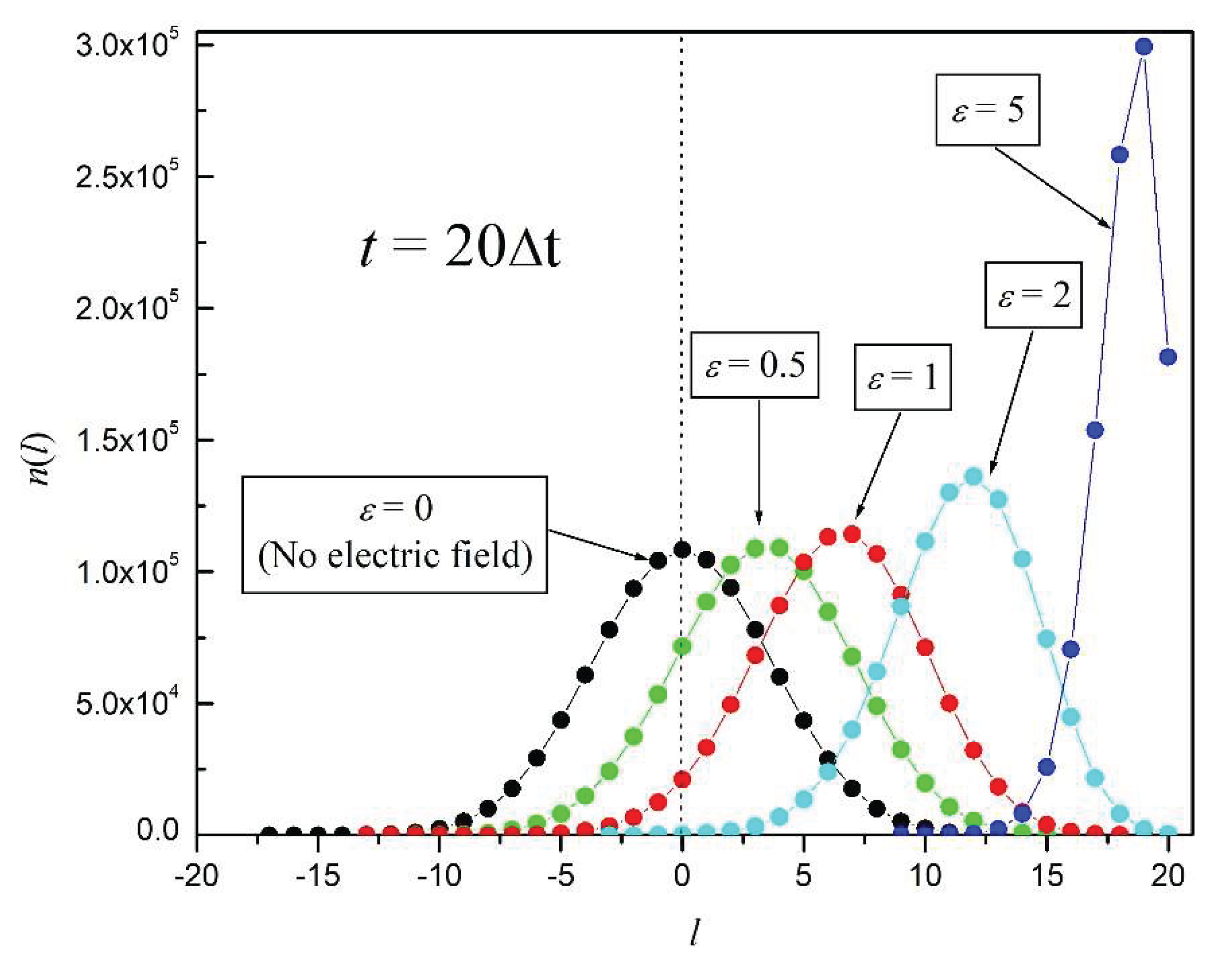
Figures 6a – 6e show the time evolution of n(l) for ε = 0, 0.5, 1, 2, and 5, respectively. The plots correspond to times t = 5Δt, 10Δt, 15Δt, and 20Δt, in each figure. The number of repetitions in each case is N = 106. In the absence of electric field (ε = 0), in Figure 6a we observe a typical Brownian evolution: the distributions n(l) are Gaussian distributions that spread about the origin with time [17]. For the case of a relatively small electric field (ε = 0.5), Figure 6b shows that the broadening of the distribution with time is accompanied by a slight shift to the right. As ε increases, the shift to the right increases as well. Note that for ε = 1 and 2 (Figures 6c and 6d) the shape of the distributions remains fairly symmetric. However, this is not the case for ε = 5: with this relatively large electric field, there is a marked predominance of particle translations to the right over translations to the left: the electric force clearly outweighs the Brownian force (thermal noise). The further the peak of a distribution moves to the right, the more pronounced the distribution asymmetry becomes and the larger the energy dissipation. This last point is true because in our model we can assume that all work performed on p is dissipated as heat, since its average kinetic energy does not increase with time: as dictated by the model’s motion rules, p does not move more than one site every unit time.
5. Applicability of the JE: A Case Study
In the previous section we have illustrated, by varying ε, the effects of the electric field magnitude on the work distributions. From this point on we will limit our attention to the ε = 1 case. As we saw above, this is a situation in which the electric field force and the random thermal noise would have similar effects.
Suppose that from t = 0 to t = τΔt the electric field acts upon particle p. If this process is repeated N times, the average work, according to Equations (5) and (9), will be
By applying Eq. (10) we get:
As explained above, all work performed on p is dissipated as heat, since the average kinetic energy of p does not increase with time. Furthermore, we can consider that all sites are equivalent. Thus, we can assume that the free energy of our system remains constant. We have then that , which is a theoretical result that is valid in the limit of an infinite number of repetitions. In contrast, for a finite number of repetitions we claim that the JE is applicable to our model only if the sum of Eq. (21) is close to unity: . In particular, we define, arbitrarily, the applicability range for the JE as which corresponds to an error tolerance of ± 0.05ε for our estimation of . (Recall that ε is the dimensionless energy unit of our system.)
According to Equations (7) and (21), and to the fact that n(Wl) = n(l), if ε = 1, then
Table 1 shows the values of obtained by using Equation (22) for times τ = 5, 10, 15, 20, 25, and 30, and for number of repetitions N = 102, 103, 104, 105, and 106. In the N = 106 case, the JE is applicable for τ = 5, 10, 15, and 20; however, for τ = 25 and 30, falls outside the applicability range (shaded values indicate that JE is not applicable). The corresponding distributions for τ = 5, 10, 15, and 20 are shown in Figure 6c, and those of τ = 25 and 30 will be presented in the following section. For N = 105 and 104 the JE applicability is limited to τ = 5 and 10. For N = 103 and 102 the JE is not applicable for the times shown.
In Table 1 we have followed the rule that if for a given N the JE is not applicable for τm, then it is assumed that the JE is not applicable for any τ larger than τm, regardless of its value. We can get a 1.00 in any instance just by chance. That is the case in the N = 104 column for τ = 30, and in the N = 103 column for τ = 15.
It is important to stress that the values shown in Table 1 are typical, and that, due to the randomness inherent to the rules of motion of our model, the applicability results might not be the same if a different set of simulations were used (we give an example of this in Section 7). Thus, we limit ourselves to say that the following trends are typically followed: 1) for a given N, the JE is not applicable above a certain τmax; and 2) this τmax decreases as N decreases.

Table 1.
for various τ’s and N’s (ε = 1). Shaded values indicate that JE is not applicable.
| τ | Number of repetitions, N | ||||
| 106 | 105 | 104 | 103 | 102 | |
| 5 | 1.00 | 1.01 | 1.02 | 0.85 | 1.68 |
| 10 | 1.02 | 1.03 | 1.00 | 1.38 | 1.09 |
| 15 | 1.01 | 1.67 | 0.68 | 1.04 | 0.34 |
| 20 | 0.97 | 1.84 | 0.66 | 0.54 | 0.61 |
| 25 | 1.19 | 2.51 | 2.54 | 0.32 | 0.25 |
| 30 | 0.77 | 0.84 | 1.05 | 0.23 | 0.30 |
6. Dominant and Typical Distributions
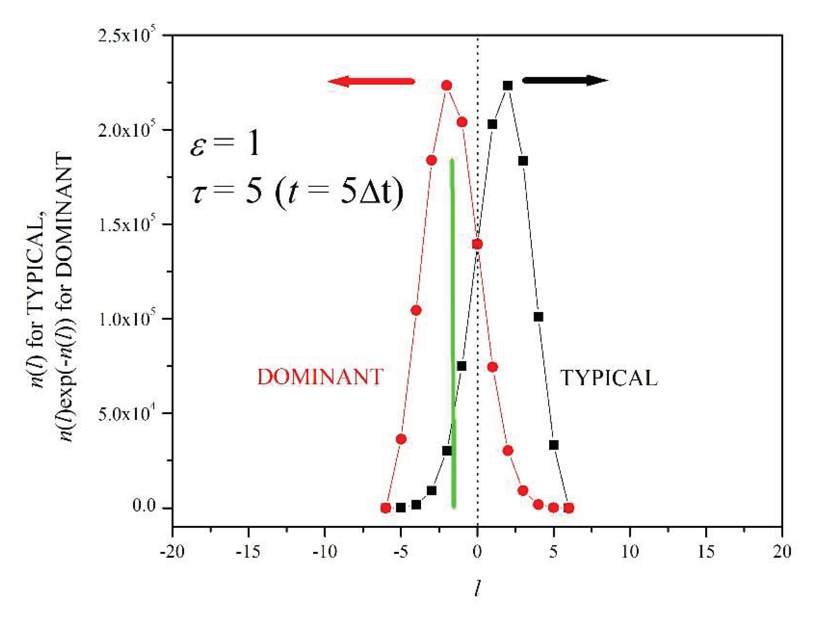
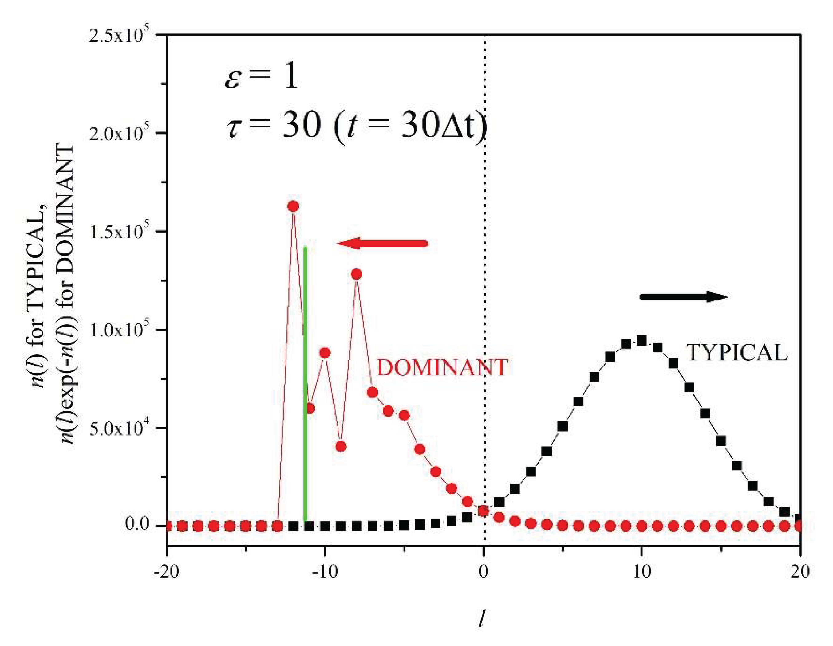
In this section we study the time evolution of the typical and dominant distributions for ε = 1 and N=106. The N = 106 column of Table 1 lists the corresponding values. The black curves (right) in Figures 7a-f represent the n(l) distributions for dimensionless times τ = 5, 10, 15, 20, 25, and 30, respectively (Figure 6c shows the same curves for τ = 5, 10, 15, 20). These curves will be called typical distributions because they peak approximately at l’s that correspond to the average work value, given by Equation (20) [11,16]. The red curves (left) correspond to the exponential expression
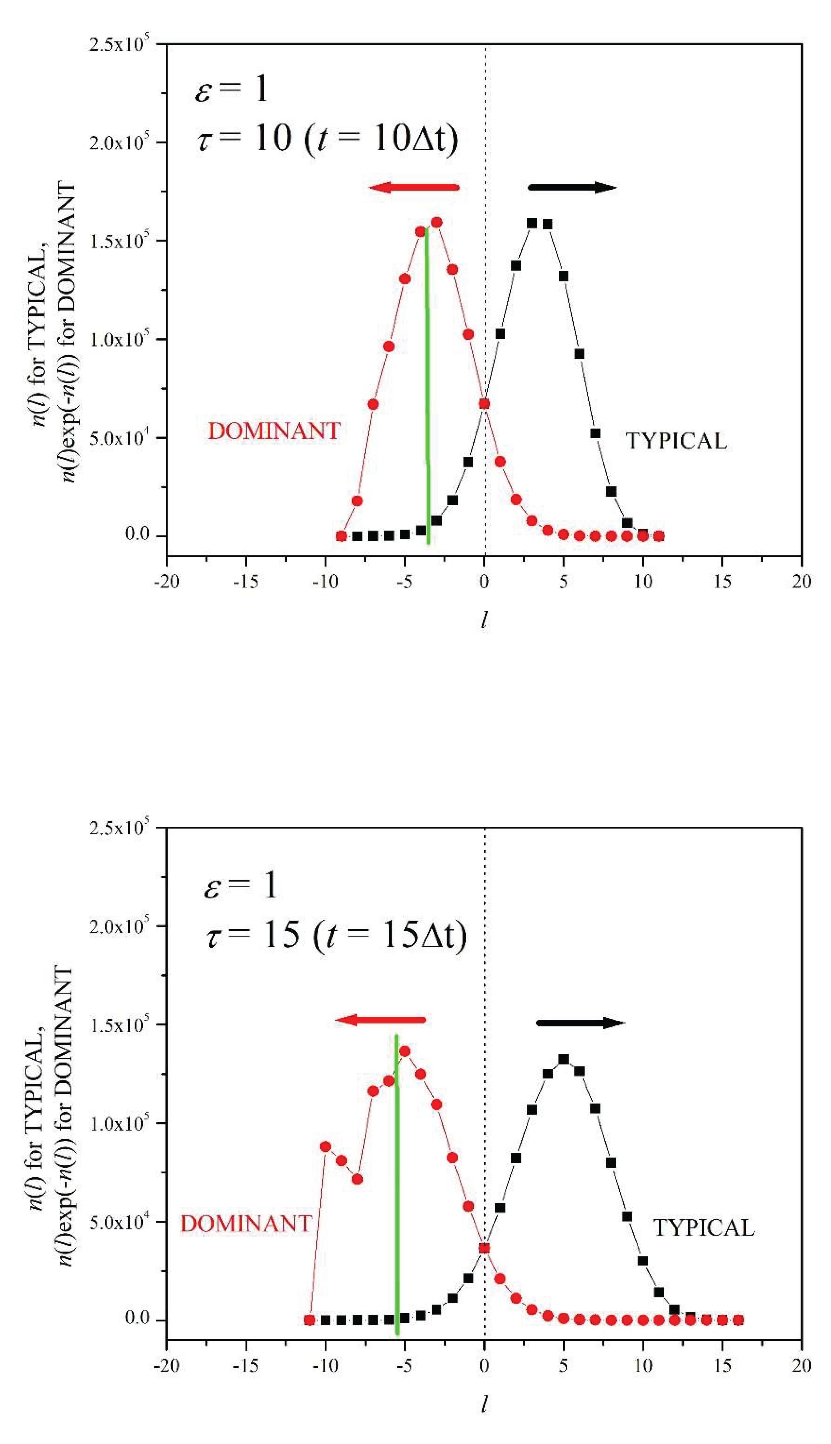
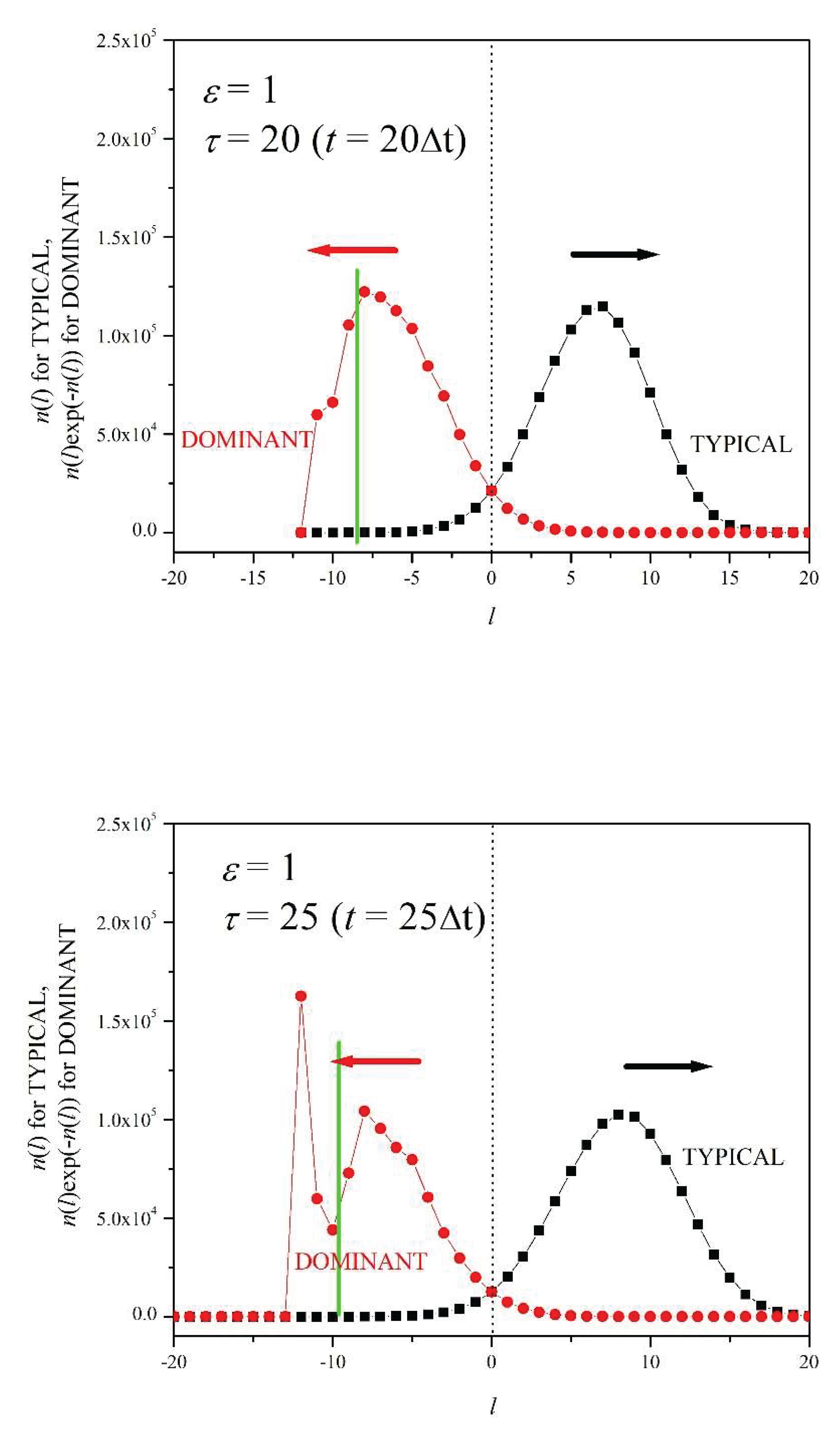
where we have used Equations (7) and (19). The work values Wl (= lε/β) at which peaks are the most important in the evaluation of the sum in Equation (21), as explained in the Introduction. Thus, we will denote the red curves (left) as dominant distributions [11,16]. Figures 7a – f show that, as τ increases, typical and dominant distributions move apart, and that the number of events, n(l), within the dominant distribution becomes a smaller fraction of N = 106. As we will see, the number of events within the dominant distribution can become several orders of magnitudes smaller than number of events within the typical distribution. That is why dominant events are known as rare events [11,16]. Figure 7a shows that at τ = 5, both the dominant and typical distributions have a nearly symmetric shape (for the dominant distribution this symmetry is highlighted by the green line at its center). At τ = 10 (Figure 7b) the distributions continue to separate, moving in opposite directions with time, as indicated by the arrows. For τ = 15, the dominant distribution has taken a noticeably asymmetric shape: its left half is irregular, since in this region n(l) is quite small. As the number of instances under the dominant distribution becomes smaller, the randomness implicit in our model becomes more evident. Figures 7d, 7e, and 7f show that both distributions keep separating as time passes and that the dominant distribution becomes increasingly more irregular; here, the green line simply indicates an estimation of where the center of symmetry would be had the symmetry not been destroyed.
We see that the more symmetric the dominant distributions are, the better the approximation by the JE to ΔF is (see column N = 106 in Table 1). The dearth of instances that qualify as rare events (those close the peak of the dominant distribution) is responsible for the unevenness of the left half of the dominant distributions for τ = 25 and 30. Accordingly, Table 1 shows that if the number of repetitions is reduced, then the maximum τ for which the JE is applicable decreases. As we have pointed out, if we use another set of repetitions (with same ε and τ), most likely we will obtain a different dominant distribution curve; this will be more noticeable in the case of an irregular distribution.
Figure 7.
Figure 7. a. Typical and dominant distributions for τ = 5 (ε = 1 and N = 106). b. Typical and dominant distributions for τ = 10 (ε = 1 and N = 106). . Typical and dominant distributions for τ = 15 (ε = 1 and N = 106). d. Typical and dominant distributions for τ = 20 (ε = 1 and N = 106). e. Typical and dominant distributions for τ = 25 (ε = 1 and N = 106). f. Typical and dominant distributions for τ = 30 (ε = 1 and N = 106).
7. The Significance of Rare Events
We have seen that a key difficulty in evaluating ΔF by means of the JE is the poor convergence of the exponential integral in Equation (4) [16]. From a practical point of view, the events pertaining to the dominant distribution (rare events) might be too few to provide us with a statistically solid evaluation of the sum in Equation (21), considering the random nature of the processes under consideration.
To illustrate the significance of rare events in evaluating by means of Equation (21), let us consider the case with ε =1, τ = 20, and N =106 (Figure 7d). Table 2 lists the values of l and the corresponding n(l) (the range -20 ≤ l ≤ 20 encompasses all possible values of l for τ = 20). Notice the great difference between the number of events around the typical peak, say n(l=6) + n(l=7) + n(l=8) = 334207, and the number of events around the rather uneven dominant peak, say n(l=-11) + n(l=-10) + n(l=-9) = 17. Thus, in this example it is about 20000 times more likely that a simulation results in an l within the typical peak than within the dominant peak: the events belonging to the dominant peak are truly rare, and their outsized effect on the JE calculation originates from the exponential in Equation (22). A point we wish to highlight here is that, in contrast to the typical peak, a small variation in the dominant peak will have a large effect on the calculation of . To illustrate this, let us move the four counts belonging to l = -11 and -10 to l = -9. Thus, now we have n(l=-9)=17, n(l=-10)=0, and n(l=-11)=0. Recalculating we obtain 0.85, and not 0.97 (see Table 1). Reshuffling four counts (out of a total of one million) within the dominant peak results in a big change on the value of ! It is in this sense that rare events are dominant. The random nature of rare events is responsible for large statistical inaccuracies.
If we ran several more sets of N = 106 repetitions of the same process, we would likely obtain n(l) distributions that would differ, to varying extents, from the one shown in Table 2. (We ran five more sets of N = 106 simulations, with ε = 1 and τ = 20, and obtained the following values for : 1.06, 0.92, 0.89, 1.06, 1,03; that is, two of these lie outside the applicability range.) Therefore, as we have indicated, the data shown in Table 1 must be considered as typical. The probability of reproducing Table 1 by repeating the whole set of simulations multiple times is very low; however, most likely the new tables would display similar patterns of shaded areas (indicating the applicability or not of the JE). If we were to increase N by several orders of magnitude, we would observe that the shaded area would recede, and that would approach unity in more cases. By increasing N we obtain a more robust statistics at the dominant peak (the relative error of n is proportional to ). But regardless of how large N is, we can always find a larger τ for which the JE is not applicable.
8. Conclusions
The Jarzynski’s equality is a theoretical result that allows us to calculate free energy differences from exponential integrals of work values. These work values can result from processes that drive a system through far-from-equilibrium states. A main difficulty in applying this equality to practical situations is the poor convergence of the aforementioned exponential integral. This is due to the relatively small number of work values from realizations known as rare events, which in spite of being significantly outnumbered by typical events, have a dominant role in the numerical evaluation of free energies.
To have a simple picture of rare events, we have used a stochastic thermodynamic model of an electrically charged Brownian particle. Work was done on the particle by a constant electric field. The simplistic rules of motion made it possible to generate work distributions of large number of work values. Graphical and numerical analyses of work distributions permitted us to demonstrate the dominant role of rare events, as well as their dependance on the number of realizations, work rate, and duration of the work process. The same type of analysis along the lines followed in this paper can be applied to calculations of free energy differences from experimental data or simulations with more realistic models to assess their reliability. Are they reproducible results? Are they just typical? Or merely random?
Appendix
In Section 3 we have shown that the probability ratio P+/P– is given by Equation (18). Here we present a sketchy derivation of this ratio, based on the assumption of the validity of the fluctuation theorem (FT). There exist slightly different versions of the FT, though all of them are a direct consequence of the principle of microscopic reversibility [6,7,10,18]. The first derivations of the FT were of a dynamical nature, where a reversible system is in contact with a thermostat [18,19,20]. However, as Crooks points out in Reference 18, a derivation based on stochastic dynamics presents fewer difficulties. We have followed such stochastic dynamical approach in defining the Markovian rules of motion of our model.
Consider a system with a dynamics that obeys the principle of microscopic reversibility, in contact with a thermal bath at temperature T [6,7,10,18]. Assume that the system releases to the thermal bath an amount of heat Q when it transitions from a state A to a state B. The reverse process, where the system retraces the exact trajectory in the opposite B-to-A direction, involves the same amount of heat but now being transferred from the heat bath to the system (a consequence of microscopic reversibility). Let PA→B be the probability of the system going from state A to state B and let PB→A be the probability of the opposite transition. By assuming microscopic reversible dynamics, the FT asserts that these probabilities are related by the following expression:
In our model, we regard the system as the positively charged particle p and the thermal bath consists of the surrounding atoms or molecules. The forces acting on p originate from the thermal noise and the electric field. Assume that p is at site x’ at t = t’. Let P+ be the probability of p moving to x’+∆x at t = t’+∆t, and let P– be the probability for the reverse transition. The dissipated energy, as heat transferred to the thermal bath, when the p moves one unit length ∆x to the right (left) is equal to qE∆x (–qE∆x). Thus, from Equation (24):
where we have used Equation (17).
Adopting symmetric expressions for the probabilities that obey Equation (25), we arrive at Equations (15) and (16).
Funding
This research received no external funding.
Data Availability Statement
Not applicable.
Conflicts of Interest
The author declares no conflict of interest.
References
- Callen, H.B., Thermodynamics and Introduction to Thermostatics, 2nd Edition, John Wiley & Sons, USA (1985).
- C. Bustamante, J. Liphardt, F. Ritort, “The nonequilibrium thermodynamics of small systems,” Phys. Today 58(7), 43 – 48 (2005). [CrossRef]
- G. Hummer, A. Szabo, “Free energy reconstruction from nonequilibrium single-molecule pulling experiments,” Proc. Natl. Acad. Sci. USA 98, 3658 – 3661 (2001). [CrossRef]
- J. Liphardt, S. Dumont, S. B. Smith, I. Tinoco Jr, C. Bustamante, “Equilibrium Information from Nonequilibrium Measurements in an Experimental Test of Jarzynski Equality,” Science 296, 1832 – 1835 (2002). [CrossRef]
- G. M. Wang, E. M. Sevick, E. Mittag, D. J. Searles, D. J. Evans, “Experimental Demonstration of Violations of the Second Law of Thermodynamics for Small System and Short Times Scales,” Phys. Rev. Lett. 89, 050601 (2002). [CrossRef]
- C. Jarzynski, “Equalities and Inequalities: Irreversibility and the Second Law of Thermodynamics at the Nanoscale,” Annu. Rev. Condens. Matter 2, 329 – 351 (2011). [CrossRef]
- L. Peliti and S. Pigolotti, Stochastic Thermodynamics, an Introduction (Princeton Academic Press, Princeton, 2021).
- C. Jarzynski, “Nonequilibrium Equality for Free Energy Differences,” Phys. Rev. Lett. 78, 2690 – 2693, 1997. [CrossRef]
- G.E. Crooks, “Nonequilibrium Measurements of Free Energy Differences for Microscopically Reversible Systems,” J. Stat. Phys. 90, 1481 – 1487, 1998. [CrossRef]
- P. Gaspard, The Statistical Mechanics of Irreversible Phenomena (Cambridge University Press, Cambridge, 2022).
- M.E. Tuckerman, Statistical Mechanics: Theory and Molecular Simulations (Oxford University Press, Oxford, 2010).
- J.G. Kirkwood, “Statistical Mechanics of Fluid Mixtures,” J. Chem. Phys. 3, 300 – 313, 1935. [CrossRef]
- R.W. Zwanzig, “High-Temperature Equation of State by a Perturbation Method,” J. Stat. Phys. 9, 1420 – 1426, 1954. [CrossRef]
- R.C. Lua, A.Y. Grosver, “Practical Applicability of the Jarzynski Relation in Statistical Mechanics: A Pedagogical Example,” J. Phys. Chem. B 109, 6805 – 6811, 2005. [CrossRef]
- H. Hijar, J.M. Ortiz de Zárate, “Jarzynski’s equality illustrated by simple examples,” Eur. J. Phys. 31, 1097 – 1106, 2010.
- C. Jarzynski, “Rare events and the convergence of exponentially averaged work values,” Phys. Rev. E 73, 046105, 2006. [CrossRef]
- P.K. Pathria, Statistical Mechanics, 2nd Edition, Butterworth-Heinemann, Oxford, UK, 1996.
- G.E. Crooks, “Entropy production fluctuation theorem and the nonequilibrium work relation for free energy differences,” Phys. Rev. E 60, 2721 – 2726, 1999. [CrossRef]
- D.J. Evans, D.J. Searles, “Equilibrium microstates which generate second law violating steady states,” Phys. Rev. E 50, 1645 – 1648, 1994. [CrossRef]
- G. Gallavotti, E.G.D. Cohen, “Dynamical Ensembles in Nonequilibrium Statistical Mechanics,” Phys. Rev. Lett. 74, 2694 – 2697, 1995. [CrossRef]
Figure 6.
Figure 6. a. Evolution of n(l) with time for ε = 0 (N = 106). b. Evolution of n(l) with time for ε = 0.5 (N = 106). c. Evolution of n(l) with time for ε = 1 (N = 106). d. Evolution of n(l) with time for ε = 2 (N = 106). e. Evolution of n(l) with time for ε = 5 (N = 106).
Figure 6.
Figure 6. a. Evolution of n(l) with time for ε = 0 (N = 106). b. Evolution of n(l) with time for ε = 0.5 (N = 106). c. Evolution of n(l) with time for ε = 1 (N = 106). d. Evolution of n(l) with time for ε = 2 (N = 106). e. Evolution of n(l) with time for ε = 5 (N = 106).
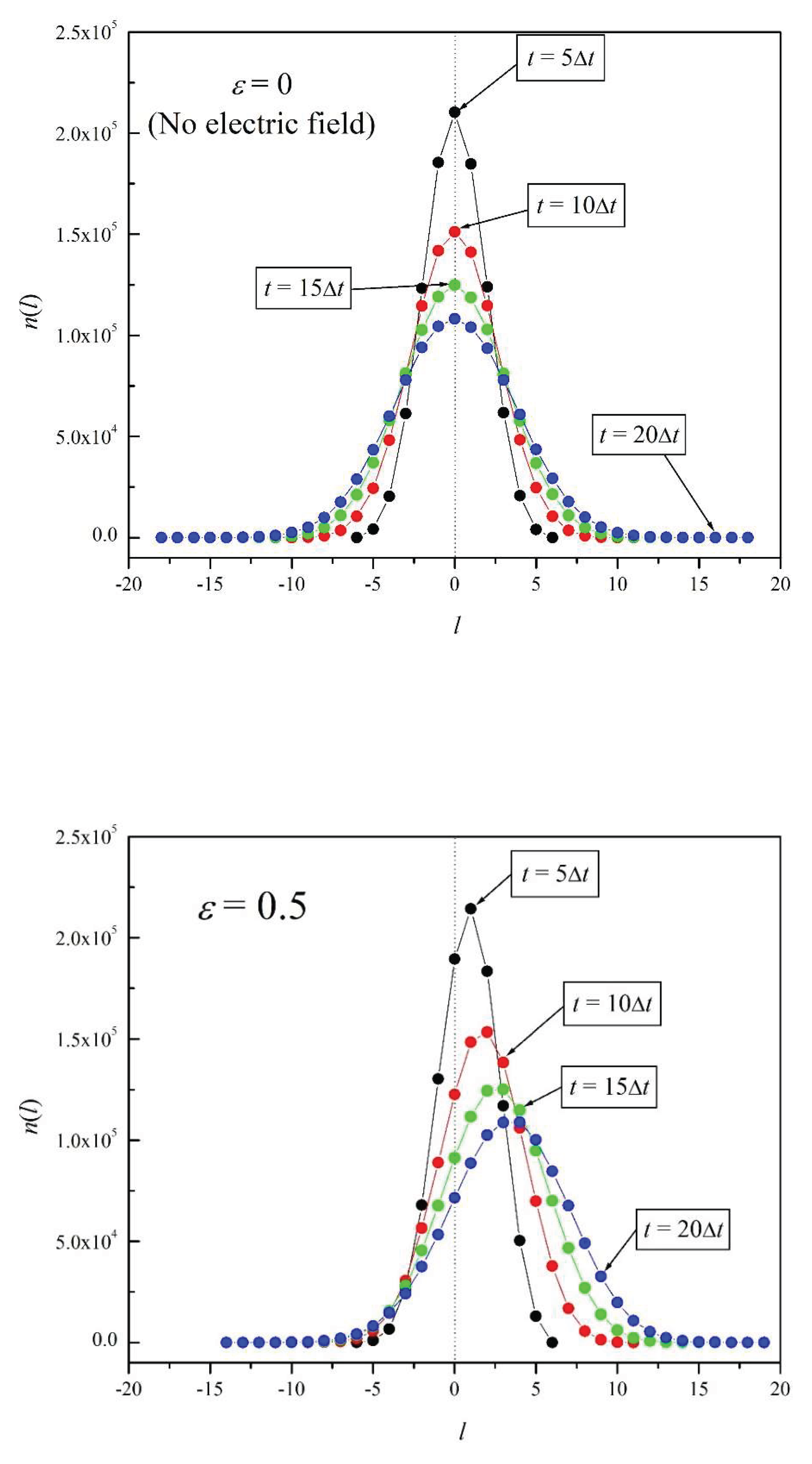
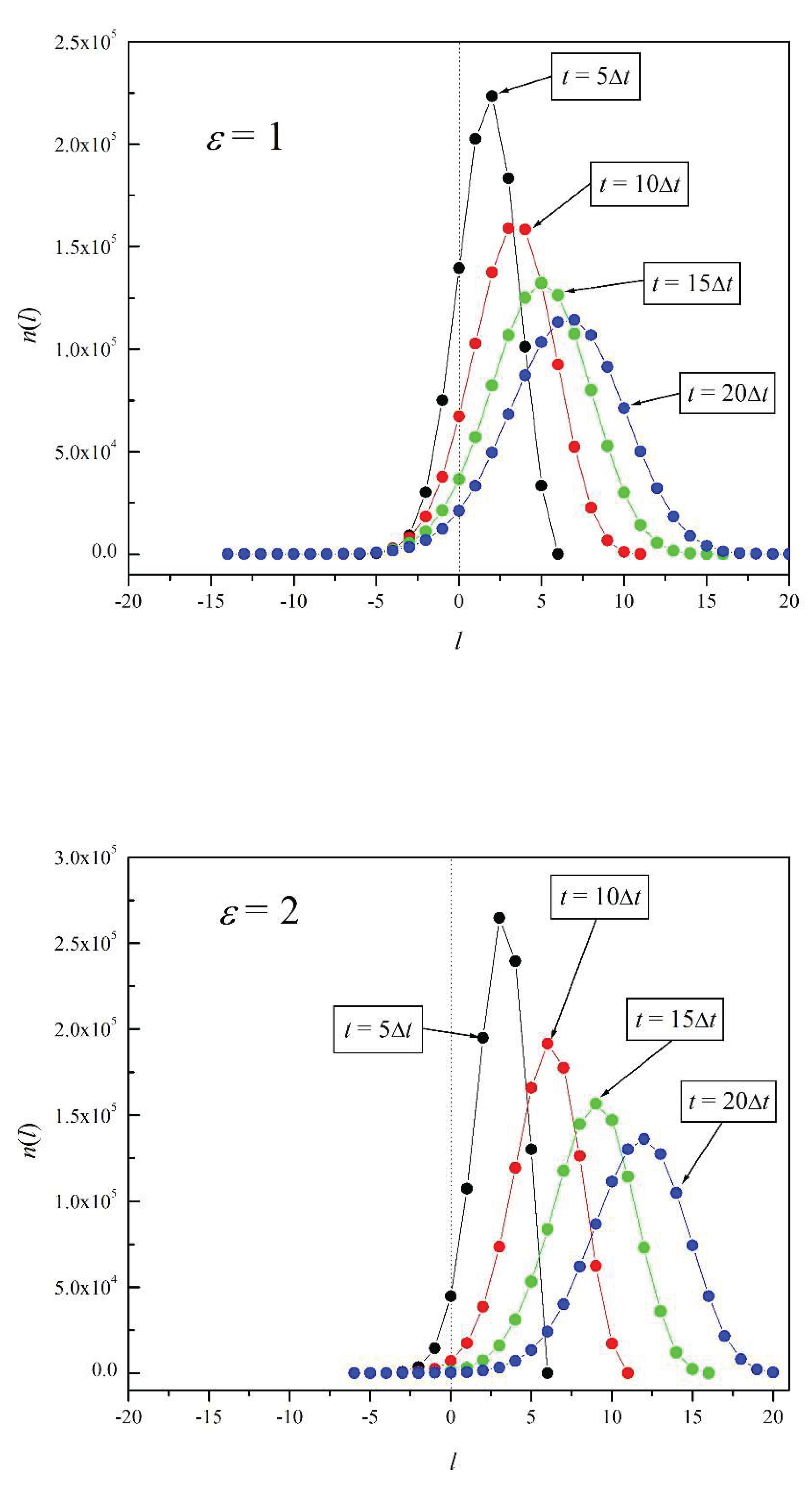
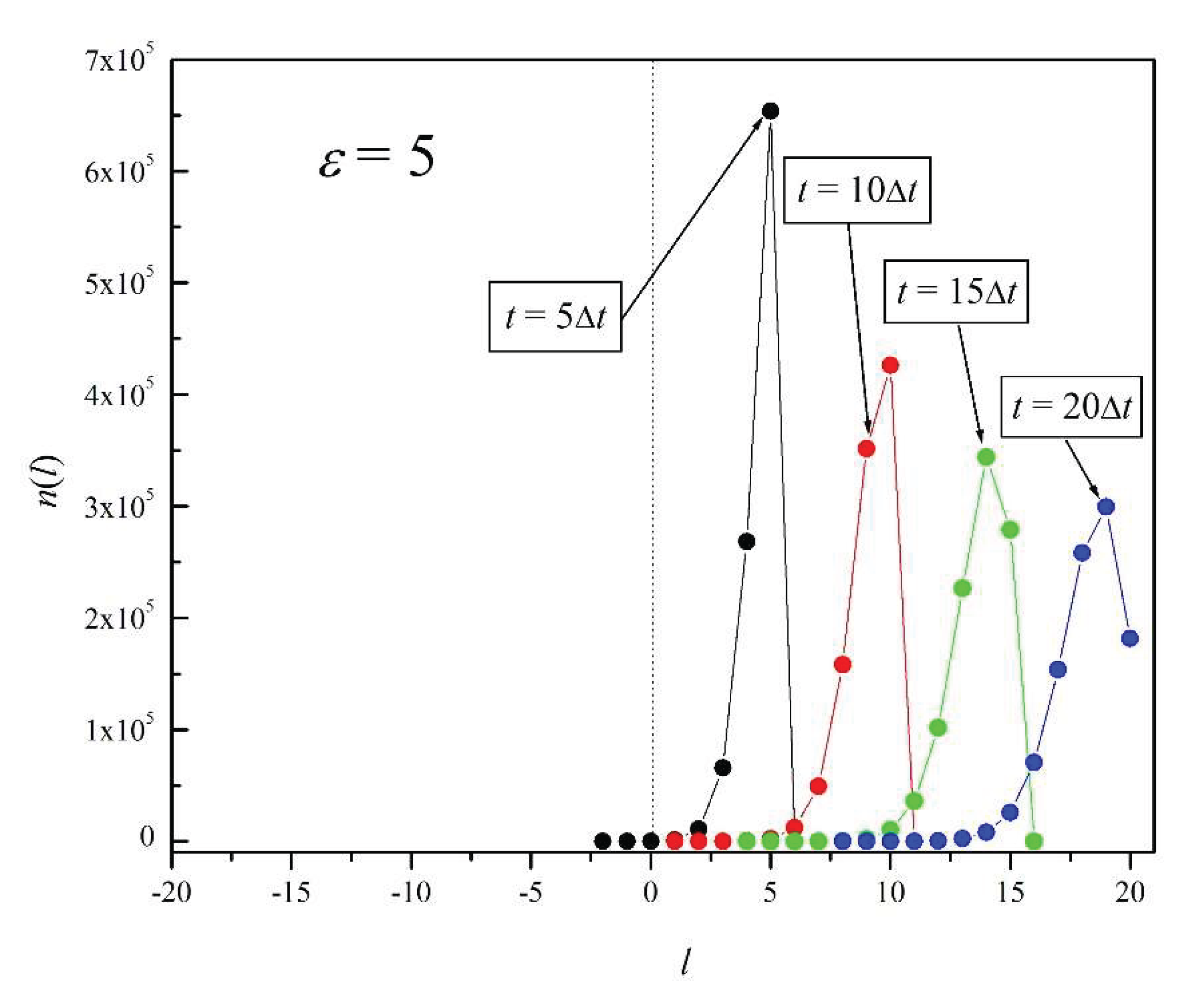
Table 2.
n(l) as a function of l for ε =1, τ = 20, and N =106.
| l | n(l), or n(Wl) |
| 20 | 1 |
| 19 | 26 |
| 18 | 77 |
| 17 | 439 |
| 16 | 1480 |
| 15 | 3824 |
| 14 | 8815 |
| 13 | 18136 |
| 12 | 31900 |
| 11 | 49941 |
| 10 | 71036 |
| 9 | 91199 |
| 8 | 106673 |
| 7 | 114720 |
| 6 | 112814 |
| 5 | 103123 |
| 4 | 87327 |
| 3 | 68598 |
| 2 | 49875 |
| 1 | 33418 |
| 0 | 21263 |
| -1 | 12440 |
| -2 | 6734 |
| -3 | 3448 |
| -4 | 1549 |
| -5 | 698 |
| -6 | 279 |
| -7 | 109 |
| -8 | 41 |
| -9 | 13 |
| -10 | 3 |
| -11 | 1 |
| -12 | 0 |
| Total | 106 |
Disclaimer/Publisher’s Note: The statements, opinions and data contained in all publications are solely those of the individual author(s) and contributor(s) and not of MDPI and/or the editor(s). MDPI and/or the editor(s) disclaim responsibility for any injury to people or property resulting from any ideas, methods, instructions or products referred to in the content. |
© 2025 by the authors. Licensee MDPI, Basel, Switzerland. This article is an open access article distributed under the terms and conditions of the Creative Commons Attribution (CC BY) license (http://creativecommons.org/licenses/by/4.0/).
Copyright: This open access article is published under a Creative Commons CC BY 4.0 license, which permit the free download, distribution, and reuse, provided that the author and preprint are cited in any reuse.


