
Submitted:
09 June 2025
Posted:
10 June 2025
You are already at the latest version
Abstract
Network-on-Chip applications’ performance and efficiency depend on task allocation and message routing, which are complex problems. In this work, we propose to use the Hungarian algorithm to dynamically route messages with the minimal cost, i.e. minimizing the communication times while consuming the least energy possible. To meet the real-time constraints coming from requiring results at each flit transmission, we also suggest a hardware version of it, which reduces processing time by an average of 42.5% with respect to its software implementation.
Keywords:
Dynamic NoC routing
; hardware Hungarian algorithm
; optimal message routing
1. Introduction
A Network-on-Chip (NoC) application is a collection of tasks that run in different processing elements (PE) and communicate with each other as defined by a directed acyclic graph (DAG).
Once PEs are allocated to tasks, messages over the network must be routed so that they can communicate with each other. Transmission of data requires an amount of energy proportional to the distance of the PEs where the sending and receiving tasks are.
The network can handle several message transmissions at the same time if they use different nodes, and the transmissions can also go over different routes. The network manager should look for the best routes for the required transmissions at a given time.
In this network, a (communication) task is transmitting a message from its source node to its destination, and a resource is the route followed by the message packets to reach its destination.
Choosing the best routes to consume the least power possible requires assigning the pending communication tasks at a given instant to the resources that minimize the overall distance of the transmission routes. In other words, minimizing the energy consumption of communications in a NoC requires solving an assignment problem every time a new set of tasks arises. This problem consists in assigning communication tasks to resources so that the cost of the assignment C is minimum:
where is the cost of assigning task i to resource j; and a task is a transmission from a source to a destination, according to the DAG of the application. The assignments must be unique, i.e:
In this case, , since there is at least one route per each task. The right values for can be found iteratively by looking for the minimum value in each row of A. This greedy approach works pretty well for , but the results strongly depend on row ordering. However, the Hungarian algorithm (HA) [27] has no dependencies on the order of the rows at the price of solving the same problem in . Fortunately, with , complexity gets closer to that of the greedy approach.
For example, an application with the DAG shown in Fig. Figure 1 (left) has 9 edges, thus 9 possible communication tasks. The application tasks can be placed at a 3x3 NoC as shown in Fig. Figure 1 (right), which allows them to communicate in a hop. Anyway, in this example, we shall assume that the NoC uses a wormhole type of communication, that the PE’s network interfaces have dual ports to connect to the horizontal and the vertical lines close by, and that the routers configure the corresponding crossbars in accordance with the communication tasks’ paths. Note that the entire horizontal or vertical bus lines are occupied for the duration of the transmissions, regardless of which sections are actually used.
For this example, there are 28 different paths that can be grouped into 13 resources, each being a set of paths that represent the possible routes that use some of the lines that also use the longest in the set.
At some given moment, the application requires communication tasks , , , and , thus the network manager needs to map them to appropriate routes to minimize bus usage.
Table 1 shows the number of lines, that is, the cost, that are used to perform each of these tasks with the available resources (only the significant ones are shown). If a given resource does not contain a communication path for a given task, the cost is set to the maximum value (the number of lines) plus one (7, in this case). The assignment problem is thus to bind these communication tasks to resources such that the sum of the cost is minimum. The bindings with cost equal to 7 imply that the corresponding task will remain pending for a further assignment.
The greedy approach and the HA assign tasks and to the same resources, but they differ in the rest of the assignments. While the greedy algorithm assigns to , the HA puts the task on hold by making an assignment that costs 7 to . In doing so, the HA can assign to , which saves 2 lines for all communications. In effect, the transmission power required for these communications is proportional to in the case of using the greedy algorithm and to when using the HA.
Obviously, running the greedy procedure on all row permutations would lead to finding the minimum at the cost of exponential time complexity, which makes the HA better.
In this work, we shall explore how the HA can be used by the network manager to dynamically route communication tasks so that they are made as efficient as possible. In this case, efficiency is measured in terms of the number of lines used per communication frame and the number of waits.
Because pending communication tasks vary over time, the matrix A varies and so does the assignment matrix . However, the calculation of A for all possible tasks can be performed offline (Section II), and only the assignment problem (submatrix of A with the rows corresponding to the pending tasks) must be solved in real time.
Calculating B might require parallel implementations or hardware accelerators. In the last case, a customized processor can run a program or specific hardware can be used.
In our case, we shall build specific hardware on FPGA from a state-machine version of the HA (Section III). Indeed, modeling the HA with state machines enables an early verification of the system and makes generation of hardware description straightforward.
The result model can be synthesized on a Field-Programmable System-on-Chip (FPSoC) and further refined to cut constants in execution time, so to suit stringent real-time requirements (Conclusion).
2. Dynamic NoC Routing
As communications among tasks in an application depend on data, it is not possible to schedule data transmissions in an efficient manner offline, thus some network manager must run online to assign routes to data packets traveling the communication infrastructure.
After a short review of the literature, we shall explain our two-step approach with an off-line PE placement and computation of the resource sets and cost matrix A, and an on-line message routing process built on top of the HA.
2.1. State of the Art
Networks-on-Chip (NoCs) emerged as a scalable and flexible solution to overcome the limitations of bus-based communication in System-on-Chip (SoC) designs [2]. Benini and Micheli introduced probabilistic and structured design principles that applied the foundation for NoC development.
Subsequent research on domain-specific NoC optimisations directed to influential architectural advancements. A comprehensive survey from Bjerregaard et al. [2] exists, categorising NoC routing algorithms, performance evaluation methods, and topological types. Meanwhile, Sahu and Chattopadhyay [2] proposed application-aware mapping techniques, emphasising task placement’s impact on design latency and energy efficiency.
Routing strategies have obtained much interest and can typically be separated into the following categories:
- (1)
- Deterministic and Adaptive Routing: Conventional methods such as XY and west-first routing offer low-complexity, deadlock-free solutions. Hybrid adaptive schemes extend these methods to manage congestion while preserving correctness guarantees [2].
- (2)
- AI-Assisted Routing and Machine Learning: Reinforcement learning (RL)-based approaches [2] dynamically adapt routing decisions to handle faults and workload variations, especially in 3D NoCs. However, these methods incur additional hardware complexity and inference latency.
- (3)
- (4)
-
Software-defined NoCs (SDNoCs): SDNoCs introduce a centralised control plane for dynamic reconfiguration [10,11], improving flexibility in heterogeneous systems but often at the cost of additional control-plane latency.These are powerful in heterogeneous systems but often introduce latency because of the control-plane signalling.
In contrast to existing routing strategies, our work explores a classical algorithmic approach—the Hungarian Algorithm (HA)—to enable dynamic, energy-aware routing in NoCs. Although the HA is traditionally used for solving assignment problems, its potential for real-time routing in NoC systems remains largely unexplored. Unlike RL-based solutions, our method provides guaranteed optimal communication cost assignments with predictable execution time, making it suitable for FPGA-based NoCs with stringent real-time constraints.
This work introduces the first complete integration of the Hungarian Algorithm (HA) into a hardware-accelerated NoC environment, where it operates in conjunction with a processing element (PE) and dynamic routing infrastructure.
- (a)
- HA is embedded within a hardware-supported framework, interfacing directly with task assignment and path allocation subsystems via the NoC.
- (b)
- The algorithm is implemented in VHDL, synthesised as a comprehensive finite state machine (EFSM) and evaluated in multiple memory organisation models (SPMEM, DPMEM).
- (c)
- We prove the impact on task wait ratios and path contention by comparing HA-based routing to greedy heuristics under diverse workloads.
- (d)
- FPGA-based emulation results significantly improve execution time and communication efficiency over a CPU-based software variant.
2.2. Off-Line Processes
Each node of the application’s DAG to be implemented in a NoC must be mapped onto a PE such that data transmission is done with the least energy consumption and data contention possible. For this, the edges of the DAG must correspond to the shortest communication paths possible. Therefore, neighbor nodes should be placed in neighbor PEs.
In this work, placement has been done either manually for the example case or automatically by traversing the graph from input nodes to output nodes, level by level, in zigzag. Each level is defined by the edge distance to the primary inputs. (It is possible to obtain optimal placements for DAG whose properties have been profiled with a quadratic assignment [12] of DAG nodes to NoC PEs, but even in this case, optimality depends on the variability of communications over time.)
For a given placement, each edge in G can be covered by a set of paths in the NoC. The paths from node s to node d start at a vertical or horizontal bus port from the PE position and end at .
The generation of these paths is done by the algorithm 1, which explores all the paths from to for every edge in G. To do so, it explores in a depth-first search manner the tree of subsequent neighbor positions. If the last position of the current path corresponds to , the path is eventually stored in the path list P. Otherwise, the current path is augmented with the positions of neighbors that do not cause cycles. In this case, a path would contain a cycle if the line where the new segment would sit intersects any previous position in the path.
The new paths are stored only if they are not included in the other paths. In case some of the other paths include the new one, they are removed from the list P, and the new one is appended.
| Algorithm 1 Path generation |
|
The generation of paths from to can be improved by dynamic programming, as the set of paths between two NoC nodes and is the same as that of to if . The relative positions of the two points must be taken into account when translating one path from one set to another, and all the paths that would use segments outside the NoC must be removed from the final sets.
However, the generated paths have different lengths, and some of them can include sequences of nodes that match other shorter paths for different source and destination points. In these cases, these paths are packed into a single resource. They are incompatible among them, so they can share the same column.
After the generation of the minimum paths, the algorithm 2 packs them into groups that form the resources. This algorithm starts by sorting the paths according to the number of lines they use and, in descending length order, proceeds to create a set S with the current path and any other path included in it. In the end, the new set is appended to the resource list R.
The lists C (for counter) and B (for boundary) store the number of resources to which paths belong and the maximum number of appearances, respectively. Any time a path is inserted into a resource, the corresponding counter in C increases. If any two paths within the same resource are compatible, i.e. they share no communications lines, they must appear in another set, thus their occurrence maximums in B increase.
| Algorithm 2 Resource generation (path packing) |
|
The calculation of the cost matrix A is quite straightforward. Each position is set to the number of lines used by a path serving the connection of the edge i in or to the maximum number of lines plus one if there is no path in with origin and end points corresponding to .
2.3. On-Line Process
The assignment of resources to tasks must be done when new pending communications tasks require to do so. We assume that computing tasks send requests to the network manager in specific time frames or cycles.
In each cycle, some communication tasks, or edges of G, must be assigned to resources from such that the sum of costs is minimum.
A straightforward approach is to pair each edge with the resource that serves it at the minimum cost. Once paired, the resources are blocked for further assignments. This greedy way of proceeding works fine when the number of resources exceeds by large that of edges to be assigned. Anyway, blocking some assignments might lead to suboptimal solutions and, thus, it is much better to make them with the HA.
In fact, both algorithms perform equally well if sequential selection of minimum task-resource values leads to final solutions. In the Lua program 3 there is a for loop for the edges to be assigned and another one for the resources. The latter is inside a repeat loop that searches for the best possible assignment.
This Lua function [13] is a version of Andrey Lopatin’s[14], which is one of the most compact implementations of the HA in the literature. In contrast with other implementations, the program does not modify cost matrix A and uses auxiliary vectors to account for the row and column offsets (U and V, respectively), the indices of rows to which columns (P) are paired with, the preceding elements in the current decision-taking step (W), the minimum costs per column (L), and a Boolean value to know whether a column is already paired (T). In this case, the zero positions of some vectors are used as control values for the program, and B to store the indices of the columns paired to each row.
| Algorithm 3 The Hungarian algorithm |
|
function HA(A)
local n, m = #A, #A[1] -- A[1..n][1..m], n<=m
if n>m then return nil, 0, 0 end
local INF = 10e12 -- infinity
local start_time = os.time()
local U, V, P, W, L, T, B = {}, {}, {}, {}, {}, {}, {}
for i = 0, n do U[i] = 0; B[i] = 0 end
for j = 0, m do V[j] = 0; P[j] = 0; W[j] = 0 end
for i = 1, n do -- for each row (task) do
P[0] = i
local j0 = 0
for j = 1, m do T[j] = false; L[j] = INF end
repeat -- repeat until task assigned
T[j0] = true
local i0, delta, j1 = P[j0], INF, 0
for j = 1, m do -- for each column (resource) do
if not T[j] then -- if not assigned then
local cur = A[i0][j]-U[i0]-V[j]
if cur<L[j] then L[j] = cur; W[j] = j0 end
if L[j]<delta then delta = L[j]; j1 = j end
end -- if
end -- for
for j = 0, m do
if T[j] then U[P[j]]=U[P[j]]+delta; V[j]=V[j]-delta
else L[j] = L[j]-delta
end -- if
end -- for
j0 = j1
until P[j0]==0
repeat local j1=W[j0]; P[j0]=P[j1]; j0=j1 until j0==0
end -- for
for j = 1, m do if P[j]~=0 then B[P[j]]=j end end
return B, -V[0], os.time()-start_time
end -- function
|
Pairing an edge of G with a resource implies that no other path within can be assigned to another edge, i.e. there can be only one 1 per column in the pairing matrix B. Unfortunately, there is no guarantee that the corresponding path is compatible with another assigned path in a different column and row. Therefore, the solutions of greedy and Hungarian algorithms must be checked for compatibility. In case some assignments are incompatible because the corresponding paths in the affected resources share lines, the associated cost is set to the maximum for one of the task-resource bounds and a the assignment procedure is repeated. The loop continues until the result contains no incompatible assignments.
The complexity of the assignment problem for different NoC sizes is illustrated in Table 2, which shows the averages of several runs. In all of the cases, all the PEs of the NoC are assigned to some node of a random graph with average node fanout of 2. Each row of the table corresponds to averages of at least 25 assignment cycles in 10 or more different random DAGs (i.e. averages of 250 runs or more). The number of paths and resources (column "no. of rsrcs.") grows with the size of the NoC, although this growth is affected by the fact that local connections also have global effects, as they use the entire communication bus lines.
The probability of a communication task being requested at any time was set to , thus the average number of requests per assignment cycle (column "no. of reqs.") is relatively low, though it grows with the size of the NoC.
As expected, the greedy approach and the Hungarian algorithm perform equally well with a slight advantage for the latter. Anyway, it is worth noting that these are the results after solving conflicts among task-resource assignments. Because this conflict-solving procedure has exponential complexity, simpler strategies must be adopted.
We have tried several options to see which one let the assignment procedures reach the best values, including selecting the first one or the one with the least cost, but none was as effective as choosing the one with the highest conflict count. This eventually generates suboptimal solutions. For the example in the table, the percentages of cases where the assignment procedure is repeated (column "%iter.") grow with the size of the NoC and so does the number of iterations (column "#iter.") to reach a fully compatible assignment of resources with, typically, some waits.
Note that there is a cumulative effect of waits (i.e. unassigned tasks that remain for the next cycle), which has not been considered here. For the cases in the table, the percentages of unattended tasks go from 3.4% to 18.7%, again with the HA option being the best. However, in a real case, the sparsity of communication needs will probably give enough free cycles to absorb pending transmissions of a set of requests.
The same cases have been simulated with different probabilities of occurrence of communication tasks requests. As expected, the differences among the two methods reduce for probabilities lower than and increase for the higher ones. In fact, for , the HA outperforms the greedy algorithm by percentages ranging from 5% to 25% in all cases and factors.
Consequently, the network manager should use the iterative conflict-solving approach with HA to maximize communication resources’ usage and minimize energy consumption and waits.
3. Hardware Synthesis of the Hungarian Algorithm
As the Hungarian algorithm is the key procedure to obtain optimal assignments, it must be run as fast as possible to enable real-time operation of the network manager when assigning routes to messages.
To speed up HA execution, there are parallel implementations in CUDA [15] that take advantage of concurrently augmenting several paths (the equivalent to solving conflicts in the greedy algorithm) but none for FPGA, where it can benefit from executing one instruction per cycle.
We have used automatic hardware synthesis tools to obtain a hardware implementation of the HA from a state-based version of it. The state machine model is easily obtained from the program and the corresponding description can be synthesized to hardware straightforwardly. For this, we use our own state machine coding pattern and simulators to verify and then synthesize the HA.
3.1. Extended Finite State Machines
An EFSM is a finite-state machine whose state is extended with other variables that remember data from one instant to the next. For example, a timer that emits a signal e every time a certain period P elapses since it receives a start signal b (see Figure 2, top) would have a computational model represented by a state machine (Figure 2, bottom) with two main states (WAIT and COUNT) and an additional variable C that stores the number of pending cycles in the COUNT state and which constitutes the extension to its main state. The input signal b and the output e are events that are only present or active (i.e., true or 1) for a specific instant, while the input signal P contains a value that is continuously present, i.e. at each instant, although its value is only considered at the same instant when .
It must be kept in mind that, from a functional point of view, the duration of these instants is not defined, and, in fact, it can be 0, fixed (unit delay) or variable. In the case of the example, it must be known, constant, and linked to a specific period which, in a hardware implementation, would be the period of the cycles of the base clock (or some exact multiple).
To avoid the problem of circular dependencies in the same instant, only Moore-type machines are allowed. In a Mealy machine, a circular dependence occurs when an output signal is connected in an immediate manner to an input signal. Typically, this can occur when multiple state machines whose outputs do not depend exclusively on their extended state are combined.
Despite the underlying model being Moore, it is possible to benefit from the advantages that Mealy machines provide by linking actions to transitions. However, as can be seen in the transitions from the WAIT state, the immediate assignment (that is, made at the beginning of the same state) to the output signal e depends exclusively on the extended state, that is, the main state and C. Therefore, it is a Moore machine (the outputs depend only on the state) but with the advantage of being able to express changes in the outputs depending on conditions of the state variables, as if it were a Mealy machine. In the example, the output e does not depend on any input signal, only on the state variable C.
Although not shown here, EFSM can include decision trees to represent complex transitions, can be combined in parallel, and can share state variables, that is, memory.
Hierarchy is implemented by combining several state machines in parallel that communicate through a protocol in which a master and a slave are defined.
The verification of this type of machines must include not only that they are Moore, but that there are no unwanted final states, that all states can be reached from the initial one, and that the conditions of the output arcs of the nodes that represent the states cover all cases and do not overlap with each other.
To illustrate how easy it can be for failures to go unnoticed, an error of this nature has been left in the diagram in Figure 2: The state machine is correct with P and C being integer values and . With values of , the conditions of the COUNT output arcs do not cover the case.
Although these basic properties of the model can be checked for each EFSM, maybe after homomorphic transformation of some expressions and variable values limited to low-cardinality sets, they must be simulated to verify that they behave as expected, at least for the tested cases.
3.1.1. Software simulation of EFSM
EFSM networks can be simulated in SW. In this case, EFSM diagrams are translated into program objects whose behavior is simulated by a simulation engine.
In our case, we use C/C++, Python or Lua, and translation is done by matching EFSM elements with programming pattern elements [16]. With this programming paradigm, the execution of the program is regulated like that of a state machine, and, to do so, it must include state variables whose value is used to determine what code must be executed in each cycle [17] and a main loop or superloop [18] that is responsible for repeating cycles and acts, in fact, as its execution engine.
Each state machine is constituted as an object of a class that has its space for data and methods for its initialization, the reading of input data, the calculation of values of the next state, the update of the current state values, and the writing of output data, among others.
The network of EFSM to be executed in parallel is represented by a System object, whose class methods call the components’ homonymous ones. This object is responsible for the communication among the system’s components and holds the common shared data. As for the timer example and the HA case, the system would be made of a single EFSM.
3.1.2. Hardware description synthesis of EFSM networks
Like the software synthesis, the hardware synthesis starts from the behavior graphs of the corresponding EFSM and can be carried out in a few steps in a simple and systematic way.
The hardware description in VHDL (VHSIC hardware description language) that is used separates the computation of the next state and the actions corresponding to the current EFSM state in different concurrent processes [19]. In fact, the code obtained is very similar to that of the software, which also separates the computation of the next extended state from that of the immediate output signals.
This type of organization makes possible optimizations by downstream hardware synthesizers difficult, for which it may be better to integrate these processes into a single algorithm.
In the first case, each process deals with a specific aspect of the state machine. One of them describes the sequential part of the machine and is responsible for generating the necessary registers for states and variables, and for establishing the event that determines the loading of the registers that store the extended state. This process must include an asynchronous reset signal for the state machine.
A second process handles transitions between states, i.e., it computes the value of the next extended state[20]. Since it is a combinational process, it must contain assignments for all possible values of the state and variables. Indeed, there should be an initialization block for all of them before specific value assignments. This prevents synthesizers from generating memory elements (latches) to hold previous values, which would typically be done, particularly when using data types suitable for synthesis such as std_logic.
The third and last process is responsible for setting the value of the outputs based solely on the extended state (Moore). It could also be done based on the state and value of the inputs (Mealy), but this might lead to possible combinational feedback when combining different state machines and, therefore, we do not use this possibility.
In this case, a VHDL code style is promoted that is easy to generate but can be refined to achieve some optimization that may be necessary according to the requirements of each specific module.
Although it is possible to refine the VHDL code to obtain more compact, faster or lower consumption versions than the original, we looked for a coding style that enables a rapid first implementation.
3.2. State-based version of the Hungarian Algorithm
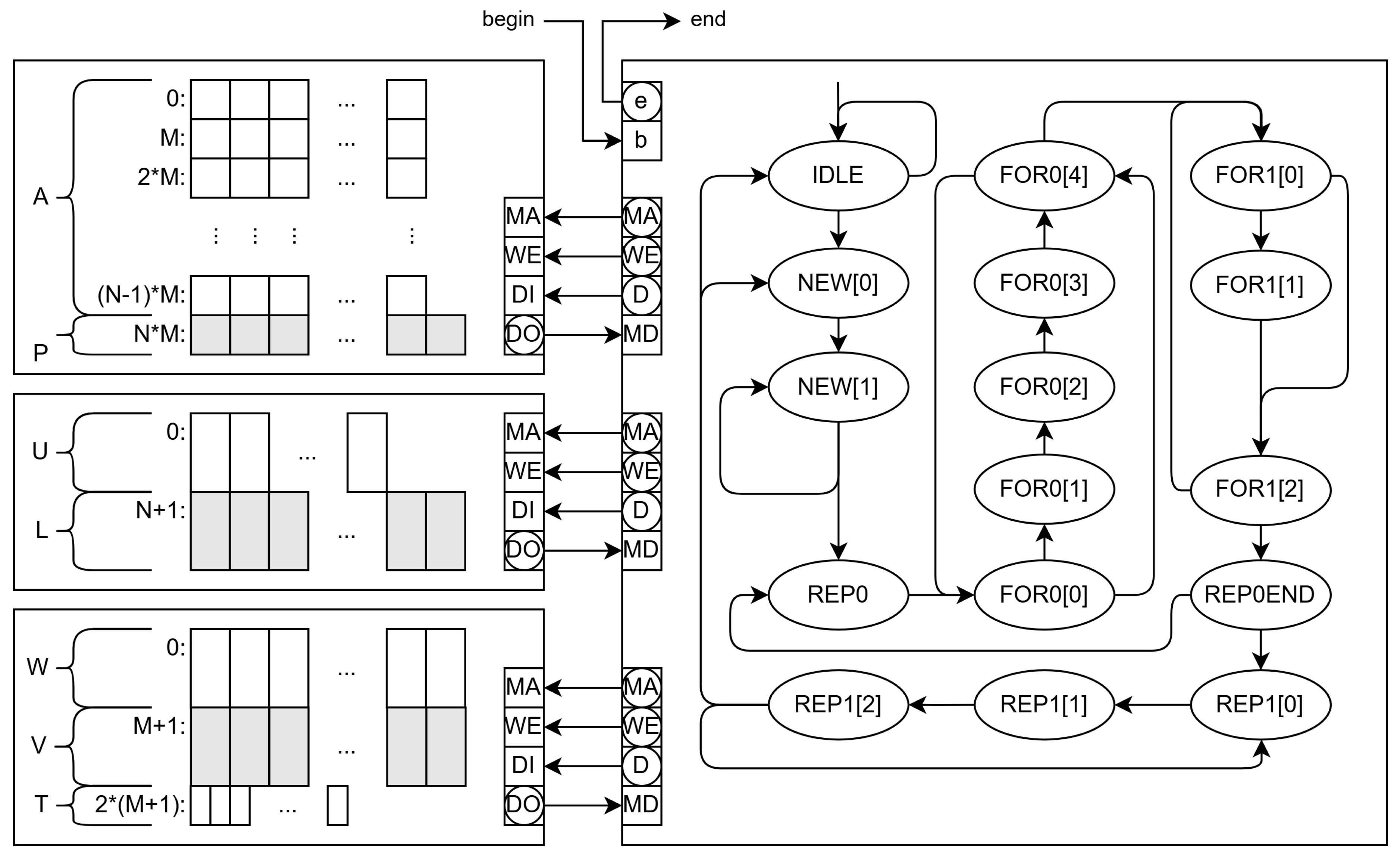
The program in 3 is transformed into an EFSM to make its software and hardware synthesis feasible. Communication between the network manager and the module is memory-mapped and through a handshake protocol with signals b (begin) and e (end of HA operation).
The memory contains the input cost matrix A and control data that include the list of edges to be assigned (not shown in Figure 3). The output data are the array P (pairing of a given column) and the first value of the array V (the negative value of the total cost). The memory system also stores auxiliary arrays L, V, W, U, and T.
The main states of the HA EFSM are shown in the state graph on the right of Figure 3, but the extended state variables are not shown for simplicity except for the outputs , and D, which are used for communication with the memory. In the initial state (IDLE), the EFSM waits for b be true and begin the execution by changing to state NEW[0].
The states NEW[0], NEW[1] and NEW[2] initialize auxiliary arrays in memory (the two first two for of function HA in Algorithm 3. Once finished, the state machine moves to REP0[0] and REP[1] states that correspond to the first repeat instruction and the previous setup of the extended state variables. This loop includes several for instructions and ends in state REP0END. In this state, the EFSM decides to return to REP0[0] or switch to REP1[0].
The REP1[0] is the first state corresponding to the last repeat instruction, and REP1[2] is the last state, where it decides whether to continue in the repeat loop, begin a new cycle of for a new edge (row of A), or end.
State names include an index between square brackets when they have sequences of actions that cannot be parallelized. Typically, memory accesses require two states in sequence: in the first one, the address is supplied to the memory unit, and, in the second one, the read datum is used in calculations and decision-making.
3.2.1. Single-Memory Architecture
A software version of this system, with two EFSM objects (the memory controller and the HA executor), has been programmed in Lua for its early verification, and coded into VHDL for its final implementation on an FPGA for its evaluation.
To compare the software version given in Algorithm 3 with the hardware implementation on an FPGA, we have tested them under the worst conditions for the HA, which are very dense square A arrays. This way, the differences in processing times reach the order of seconds, and are measurable for the software version. Note that, under actual NoC conditions, A has more resources than tasks to be assigned () and has a relatively low density because only a fraction of the resources can carry a given task (i.e., most of the values in A are the maximum cost plus one). As an example, an average random graph of an NoC has 128 edges, 8 tasks per cycle, and 256 resources (values from Table 2 adjusted to powers of 2), with cost matrix A sized and for the assignments.
Figure 4 shows the averages of 10 executions of the HA program on an Intel 12th gen i5-1235SU 1.3GHz processor running MS-Windows 11, and on an Altera Cyclone 10 LP FPGA. The hardware block works at 114 MHz and takes 1133 logic elements and 277 registers.
The software version is roughly ten times faster than the FPGA because of the clock frequency. In this case, because of the ratio between the two clocks, the energy consumption would be approximately the same as the product of time by clock frequency gives similar values for the two options. It is interesting to note that the same software run on an Intel processor at 3.2 GHz took roughly the same times to execute the testbench, which indicates that the bottleneck of the execution is the communication with the memory. The advantage of using the hardware block is that the memory system can be adapted to minimize this bottleneck.
3.2.2. Other Memory Architectures
The presented hardware version (SPMEM) can be improved by using a double port memory block and by splitting the single memory block into several blocks.
The double port memory enables two reads in a clock cycle and, thus, requires less states to achieve the same functionality. In this case, the memory layout is kept the same, but there are some operations that require more than two data from memory.
As the number of states is reduced (19 with respect to 25 for the single-port RAM version), so it is the circuitry, which takes up only 783 logic elements and 160 registers on a Cyclone 10 LP. This reduction also enables the double port version (DPMEM) to go 11% faster, operating at a clock frequency of 126.5 MHz (worst case).
To be able to make an instruction per clock cycle, more memory reads are needed. We have built a version with three memory blocks (TMEM) that reduces the number of states (15), as compared to the previous EFSM, and closes the gap between cycles and operations.
In this case, the number of logic elements is further reduced to 568 but the number of registers increases up to 180 with respect to the double port version. Anyway, the circuit is smaller and the wort-case clock frequency (134.9 MHz) higher than those of the previous versions.
Table 3 shows the averages of the measures of ten executions for ten random DAGs for each NoC size. Each DAG takes up all the PEs available in the corresponding NoC. As expected, the number of clock cycles decreases with the number of parallel reads. Because the circuits are smaller in the DPMEM and TMEM versions, the critical paths are also shorter, and thus the maximum clock frequencies increase.
To some extent, this frequency increase keeps the power consumption the same, but at a significant time savings. The DPMEM version is 34.5% faster than the SPMEM, and the TMEM version reaches 42.5% savings in time. These savings reach an average of 26.7% (DPMEM) and 30.9% (TMEM) for the same clock frequency, which would also imply that these versions operate at a lower power consumption.
Therefore, compared to SPMEM or the software version, the TMEM module uses hardware parallelism to achieve an increase in speed up to .
These results show that NoC implementations in FPSoC may use hardware HA modules to minimize power consumption and time to route internal messages with respect to performing the same computations in an embedded processor.
Figure 6.
Schematic of the HA EFSM (right) with three memory blocks (left).
4. Conclusions
NoC and artificial intelligence (AI) can benefit each other: AI processes depend on complex systems with intercommunicating tasks that can be implemented in NoC efficiently, while NoC mapping and routing require AI to be efficient, too.
In this work, we have approached the problem of routing messages from a conventional algorithmic perspective. Although the problem belongs to the nondeterministic polynomial-time complexity class (NP), part of the complexity is transferred to pre-runtime processes, namely the computation of all paths in the application’s DAG and their packing into the so-called resource groups. Computation of all paths is computationally viable because the target NoC are wormhole type, which reduces the exploration space significantly.
We have presented a strategy to leave the heavy computation processes (path generation and packing) away from the ones that have to be frequently run (binding communication tasks and resource packs) so that optimal assignments can be computed in real time.
As the resources are not totally independent from each other, HA is executed iteratively to cope with incompatible assignments. The probability of these assignments to occur increases with the size of the NoC, as well as the average number of iterations per assignment.
The dynamic nature of communications can be handled with frequent updates in the assignment of communication tasks and resources. We have shown that for the best case scenarios the HA behaves like a greedy algorithm, and that for the worst cases it outperforms the greedy version by up to 25%.
Therefore, it is clear that the HA is a good alternative to the greedy option for the NoC network managers to assign routes that minimize the overall time and power consumption.
In case the NoC are implemented in FPSoC, the assignment can be done by a specific hardware module in order to speed up this process.
We have implemented a compacted software version of the HA and the simulators of the equivalent EFSM versions, which had been verified against the original program and served to verify the functionality of the VHDL versions.
Due to the sequential nature of the HA, direct translation of the program to an EFSM with a single memory results in a hardware module that executes the algorithm at the same cost as its software version.
We have developed two versions with different memory architectures to show that the hardware options achieve better performances than the software. In fact, the version with three memory blocks can go at least 1.75 times faster.
In a nutshell this work emphasizes that although IA methods can undoubtedly be used for mapping and routing NoC applications, they can successfully be complemented by algorithmic methods.
Supplementary Materials
The following supporting information can be downloaded at the website of this paper posted on Preprints.org.
Author Contributions
Conceptualization, Ll.R. and A.P.; methodology, Ll.R.; software, Ll.R.; validation, Ll.R. and A.P.; formal analysis, Ll.R. and A.P.; investigation, Ll.R. and A.P.; resources, Ll.R. and A.P.; data curation, Ll.R.; writing—original draft preparation, Ll.R. and A.P.; writing—review and editing, Ll.R. and A.P.; visualization, A.P.; supervision, A.P.; project administration, A.P. All authors have read and agreed to the published version of the manuscript.
Funding
This research received no external funding.
Data Availability Statement
The raw data supporting the conclusions of this article has been generated by software that will be made available by the authors on request.
Conflicts of Interest
The authors declare no conflicts of interest.
Abbreviations
The following abbreviations are used in this manuscript:
| CUDA | Compute Unified Device Architecture |
| DAG | Directed acyclic graph |
| EFSM | Extended finite-state machine |
| FPGA | Field-programmable gate array |
| FPSoC | Field-Programmable System-on-Chip |
| HA | Hungarian algorithm |
| NoC | Network-on-Chip |
| NP | Nondeterministic polynomial time complexity class |
| PE | Processing element |
| SDNoC | Software-defined NoC |
| SoC | System-on-Chip |
| VHDL | VHSIC hardware description language |
References
- Kuhn. H.W. The Hungarian method for the assignment problem. Nav. Res. Logist. Q. 1955, 2, 83–97. [Google Scholar] [CrossRef]
- L. Benini and G. De Micheli, “Networks on Chips: A new SoC paradigm,” Computer, vol. 35, no. 1, pp. 70–78, 2002. [CrossRef]
- T. Bjerregaard and S. Mahadevan, “A survey of research and practices of network-on-chip,” ACM Computing Surveys (CSUR), vol. 38, no. 1, pp. 1–51, 2006. [CrossRef]
- P. K. Sahu and S. Chattopadhyay, “A survey on application mapping strategies for Network-on-Chip design,” Journal of Systems Architecture, vol. 59, no. 1, pp. 60–76, 2013. [CrossRef]
- Arm Limited, “ARM AMBA CHI 700 CoreLink Technical Reference Manual,” 2023. [Online]. Available: https://developer.arm.com/documentation/101569/0300/? 2: (Accessed, 2025.
- J. Jiao, R. J. Jiao, R. Shen, L. Chen, J. Liu, and D. Han, “RLARA: A TSV-Aware Reinforcement Learning Assisted Fault-Tolerant Routing Algorithm for 3D Network-on-Chip,” Electronics, vol. 12, no. 23, p. 4867, 2023. [CrossRef]
- Y. Zheng, T. Y. Zheng, T. Song, J. Chai, X. Yang, M. Yu, Y. Zhu, Y. Liu, and Y. Xie, “Exploring a New Adaptive Routing Based on the Dijkstra Algorithm in Optical Networks-on-Chip,” Micromachines, vol. 12, no. 1, p. 54, 2021. [CrossRef]
- X. Yang et al., “A Novel Algorithm for Routing Paths Selection in Mesh-Based Optical Networks-on-Chips,” Micromachines, vol. 11, no. 11, p. 996, 2020. [CrossRef]
- J. Fang, D. J. Fang, D. Zhang, and X. Li, “ParRouting: An Efficient Area Partition-Based Congestion-Aware Routing Algorithm for NoCs,” Micromachines, vol. 11, no. 12, p. 1034, 2020. [CrossRef]
- A. Scionti, S. A. Scionti, S. Mazumdar, and A. Portero, “Towards a Scalable Software Defined Network-on-Chip for Next Generation Cloud,” Sensors, vol. 18, no. 7, p. 2330, 2018. [CrossRef]
- J. R. Gómez-Rodríguez et al., “A Survey of Software-Defined Networks-on-Chip: Motivations, Challenges and Opportunities,” Micromachines, vol. 12, no. 2, p. 183, 2021. [CrossRef]
- Sahu, P.; Chattopadhyay, S. A survey on application mapping strategies for Network-on-Chip design. Journal of Systems Architecture 2013, 59, 60–76. [Google Scholar] [CrossRef]
- Ribas-Xirgo, Ll.; TAS: Task assignment solver. SourceForge, Dec. 2024. Available online: https://sourceforge.net/projects/tas/ (accessed on 12-May-2025).
- Minisini, A.; Kulkov, O. Hungarian algorithm for solving the assignment problem Dec. 13, 2023. Available online: https://cp-algorithms.com/graph/hungarian-algorithm.html (accessed on 12-May-2025).
- Yadav, S.S.; Lopes, P.A.C.; Ilic, A.; Patra, S.K. Hungarian algorithm for subcarrier assignment problem using GPU and CUDA International Journal of Communication Systems March 2019. 32, 20 March. [CrossRef]
- Ribas-Xirgo, Ll. State-oriented programming-based embedded systems’ course (In Spanish). XXIV Jornadas sobre la Enseñanza Universitaria de la Informática.
- Ribas-Xirgo, Ll. How to code finite state machines (FSMs) in C. A systematic approach 2014. [Google Scholar] [CrossRef]
- Pont, M.J. Embedded C, Pearson Education Ltd.: Essex, England, 2005.
- Ribas-Xirgo, Ll. How to implement the Hungarian algorithm into hardware. 39th. Conf. on Design of Circuits and Integrated Circuits (DCIS).
- Skahill, K. VHDL for Programmable Logic, Cypress Semiconductor, 1995.
Figure 1.
A DAG of an application and its mapping into a 3x3 NoC.
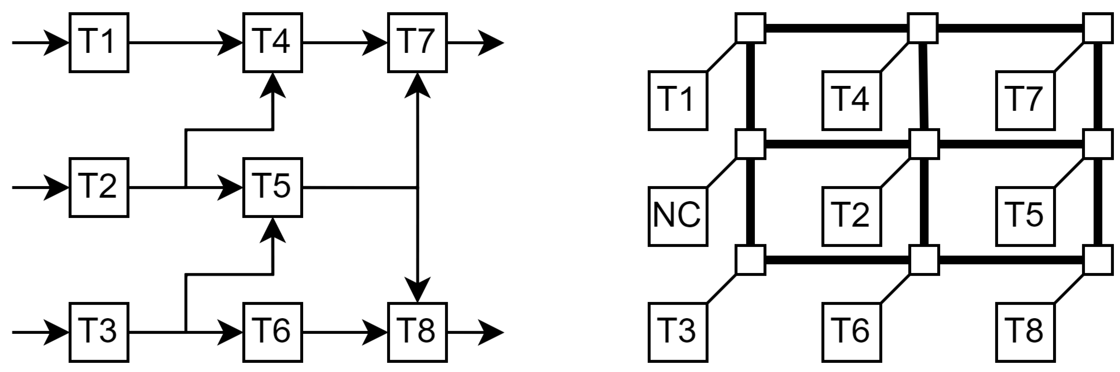
Figure 2.
Computational model of a timer controlled by a signal b that indicates the instant, or clock cycle, from which it begins to count P transitions and, with the last one, emits a positive pulse through the output signal e.
Figure 2.
Computational model of a timer controlled by a signal b that indicates the instant, or clock cycle, from which it begins to count P transitions and, with the last one, emits a positive pulse through the output signal e.
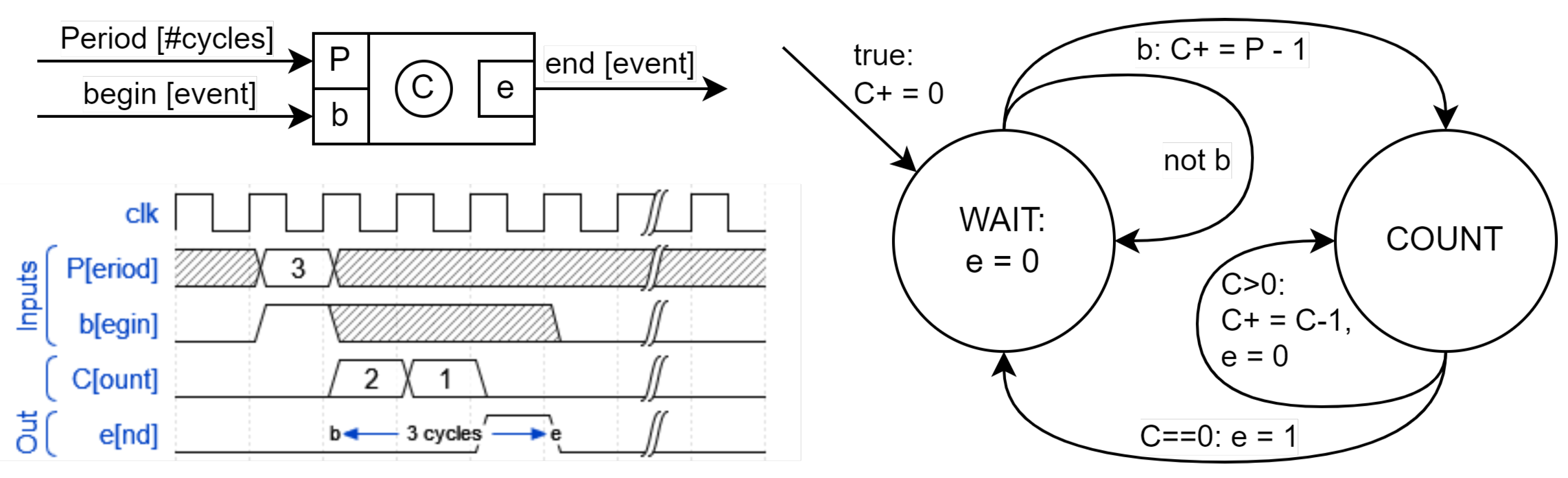
Figure 3.
Schematic of the HA EFSM (right) and of the memory layout (left).
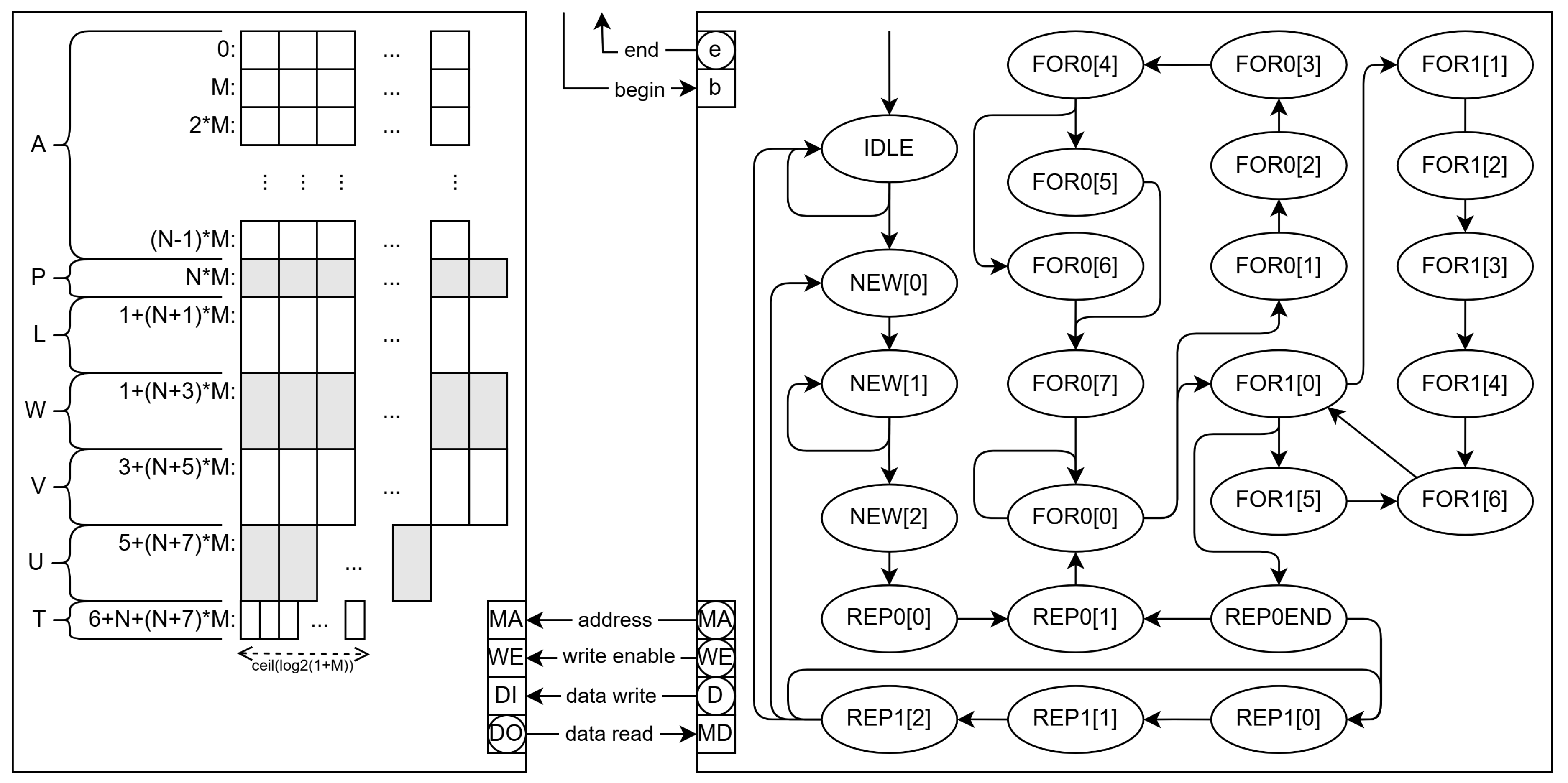
Figure 4.
Comparison between software and hardware version of the HA with respect to the problem size (square A length). The z-axis is logarithmic with units adjusted to show differences: times are shown as s.
Figure 4.
Comparison between software and hardware version of the HA with respect to the problem size (square A length). The z-axis is logarithmic with units adjusted to show differences: times are shown as s.
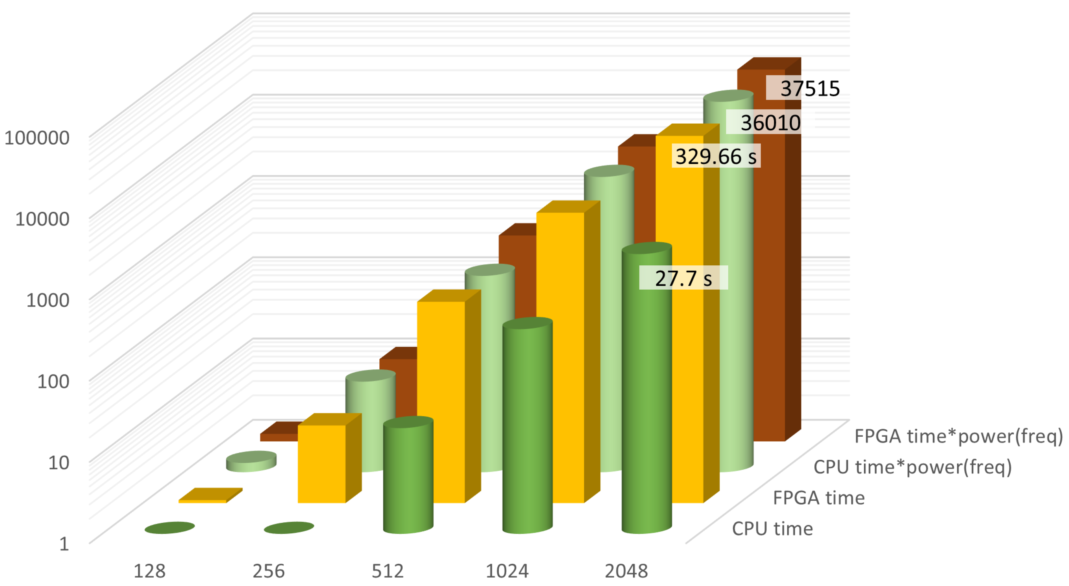
Figure 5.
Schematic of the HA EFSM (right) with a true double port memory (left).
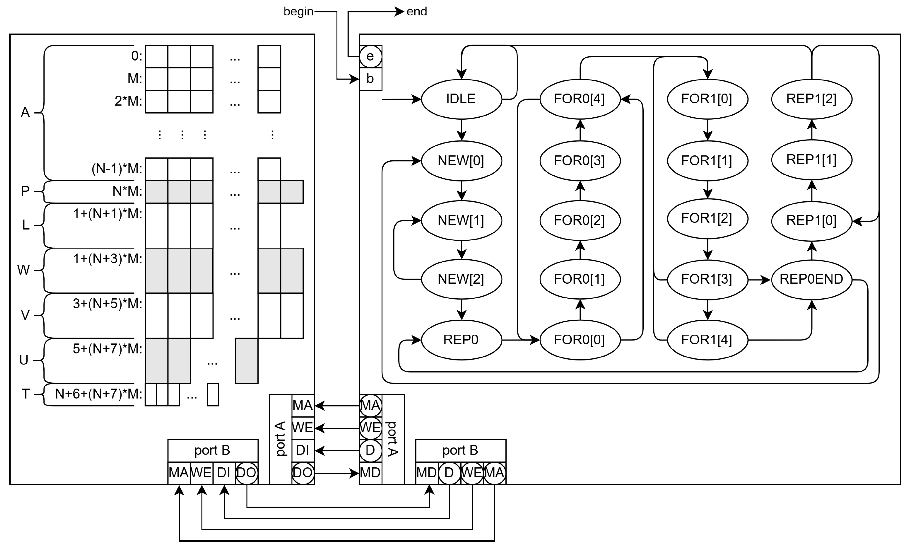

Table 1.
Task-resource table.
| … | |||||||
|---|---|---|---|---|---|---|---|
| 3 | 3 | 7 | 7 | … | 7 | ||
| 7 | 7 | 2 | 2 | … | 2 | ||
| 7 | 7 | 7 | … | 7 | |||
| 7 | 7 | 7 | … | 7 | |||
| 7 | 3 | 1 | 7 | … |
† The greedy approach takes the first available minimum value. ‡ The Hungarian algorithm proceeds the same way but looks for alternatives to minimize the sum of costs.
Table 2.
Simulation of dynamic message routing.
| NoC | No. | No. | No. | Greedy algorithm | HA | ||||||
|---|---|---|---|---|---|---|---|---|---|---|---|
| size | paths | rsrcs. | reqs. | cost † | waits | %iter. | #iter. | cost † | waits | %iter. | #iter. |
| 4x4 | 109.0 | 41.4 | 1.9 | 3.28 | 0.08 | 11.6 | 16.41 | 3.14 | 0.06 | 11.6 | 14.21 |
| 5x5 | 217.5 | 80.4 | 2.7 | 5.72 | 0.20 | 21.6 | 24.98 | 5.52 | 0.18 | 21.6 | 24.15 |
| 6x6 | 362.8 | 126.3 | 3.3 | 8.76 | 0.33 | 32.8 | 33.09 | 8.23 | 0.29 | 33.6 | 29.08 |
| 7x7 | 573.8 | 174.9 | 4.6 | 14.52 | 0.57 | 50.0 | 42.90 | 14.09 | 0.54 | 50.0 | 40.30 |
| 8x8 | 888.8 | 245.5 | 6.0 | 22.74 | 0.88 | 61.6 | 69.16 | 22.04 | 0.88 | 62.0 | 67.50 |
† Cost includes #wait .
Table 3.
Comparison between hardware implementations.
| NoC size | 113.8MHz clock cycles | 126.5MHz clock cycles | DPMEM vs. SPMEM | 134.9MHz clock cycles | TMEM vs. DPMEM | TMEM vs. SPMEM |
|---|---|---|---|---|---|---|
| 8x8 | 1866 | 1349 | 1233 | |||
| 16x16 | 8051 | 5860 | 5430 | |||
| 32x32 | 43129 | 31620 | 29597 | |||
| 64x64 | 229326 | 167246 | 158406 | |||
| 128x128 | 1238500 | 902290 | -34.45% | 860260 |
Disclaimer/Publisher’s Note: The statements, opinions and data contained in all publications are solely those of the individual author(s) and contributor(s) and not of MDPI and/or the editor(s). MDPI and/or the editor(s) disclaim responsibility for any injury to people or property resulting from any ideas, methods, instructions or products referred to in the content. |
© 2025 by the authors. Licensee MDPI, Basel, Switzerland. This article is an open access article distributed under the terms and conditions of the Creative Commons Attribution (CC BY) license (http://creativecommons.org/licenses/by/4.0/).
Copyright: This open access article is published under a Creative Commons CC BY 4.0 license, which permit the free download, distribution, and reuse, provided that the author and preprint are cited in any reuse.


