Markov Observation Models and Deepfakes

1. Introduction

Hidden Markov models (HMMs) were introduced in papers by Baum and Petrie [1] and Baum and Eagon [2]. Traditional HMMs have enjoyed tremendous modelling success in applications like computational finance (see e.g. Petropoulos et al. [34]), single-molecule kinetic analysis (see Nicolai [33]), animal tracking (see Sidrow et al. [39]), forecasting commodity futures (see Date et al. [13]) and protein folding (see Stigler et. al. [41]). The unobservable hidden HMM states ${\displaystyle X}$ are a discrete-time Markov chain and the observations process ${\displaystyle Y}$ is some distorted, corrupted partial information or measurement of the current state of ${\displaystyle X}$ satisfying the condition

$${\displaystyle P\left(Y_n\in A|X_n,X_{n-1},...,X_1\right)=P\left(Y_n\in A|X_n\right).}$$

These emission probabilities, ${\displaystyle P\left(Y_n\in A|X_n\right)}$, have some conditional probability mass function $y\to b_{X_n}\left(y\right)$.

Perhaps, the most common problems in HMM are calibrating the model, decoding the hidden sequence from the observation sequence, and real-time believe state propagation, i.e. filtering. The first problem is solved recursively in the HMM setting by the Baum-Welch re-estimation algorithm, which is an application of the Expectation-Maximization (EM) algorithm, predating the EM algorithm. The second, decoding problem is solved by the Viterbi algorithm (see Viterbi [44], Rabiner [37]), which is a dynamic programming type algorithm. The filtering problem is also solved effectively after calibration using a recursive algorithm that is similar to part of the Baum-Welch algorithm. In practice, there can be numeric problems like a multitude of local maxima to trap the Baum-Welch algorithm or inefficient matrix operations when the state size is large but the hidden state resides in a small subset most of the time. In these cases, it can be adviseable to use particle filters or other alternative methods, which are not the subject of this note (see instead Cappé et al. [7] for more information). The forward and backward propagation probabilities of the Baum-Welch algorithm also tend to get very small over time, the small number problem. While satisfactory results can sometimes be obtained by (often logarithmic) rescaling, this small number problem is still a severe limitation of the Baum-Welch algorithm. However, the independent emmission form of the observation modeling in HMM can be yet more foundamentally limiting.

The autoregressive HMM (AR-HMM) and, more generally, the pairwise Markov chain (PMC) were introduced to allow more extensive and practical observation models. For the AR-HMM the observations take the structure:

$$Y_n={\beta }_0^{\left(X_n\right)}+{\beta }_1^{\left(X_n\right)}{Y}_{n-1}+\dots +{\beta }_p^{\left(X_n\right)}{Y}_{n-p}+{\epsilon }_n,$$

(1)

where ${\left\{{\epsilon }_n\right\}}_{n=1}^{\infty }$ are a (usually zero-mean Gaussian) i.i.d. sequence of random variables and the autoregressive coefficients are functions of the current hidden state $X_n$. The AR-HMM has experienced strong success in applications like speech recognition (see Bryan and Levinson [6]), diagnosing blood infections (see Stanculescu et al. [40]) and the study of climate patterns (see Xuan [46]). One advantage of the AR-HMM is that the Baum-Welch algorithm can still be used (see Bryan and Levinson [6]).

The general PMC model from Pieczynski [35] only assumes that $(X,Y)$ is jointly Markov. Derrode and Pieczynski [15], Derrode and Pieczynski [16] and Kuljus and J. Lember [28] explain the generality of PMC and give some interesting subclasses of this model. It is now well understood how to filter and decode PMCs. In fact, Kuljus and J. Lember [28] solves the decoding problem in great generality while Derrode and Pieczynski [16] uses Baum-Welch-like recursions to produce the filter. Both Derrode and Pieczynski [15] and Derrode and Pieczynski [16] assume reversibility of the PMCs and have the observations living in a continuous space. To our knowledge the Baum-Welch rate re-estimation algorithm has not been proven in general for PMCs. Our first goal is to develop and prove this Baum-Welch algorithm for PMCs while at the same time estimating hidden initial states and overcoming the small number problem mentioned above by using alternative variables in our forward and backward recursions. Our EM resulting algorithm will apply to many big data problems.

Our second goal is to show the applicability of HMM, PMC as well as a model, called the Markov Observation Model (MOM) here, part way in between HMM and PMC in deep fake detection and generation. The key to producing and detecting deep fakes is to bring in an element that is easily calculated yet often overlooked in HMM and PMC, the Likelihood. During training as well as detection, Likelihood can be used in place of the discriminator in a Generative Adversarial Network (GAN) while simulation plays the part of generator. Naturally, the expectation-maximization algorithm also plays a key role in this deep fake application as explained below.

Our third goal is subtler. Just because the PMC model is more general than the HMM and the Baum-Welch algorithm can be extended to learn either model does not mean one should pronounce the death of the HMM. The problem is that the additional generality leads in general to a more complicated likelihood with a multitude of maxima for the EM algorithm to get trapped in or choose from. It can become a virtually impossible task to learn a global, or even a useful, maximum. Hence, the performance of the PMC model as a hidden Markov structure can be sub-optimal compared to HMM or MOM as we shall show empirically. Alternatively, the global maximum of the PMC may not be what is wanted. For these reason, we promote the MOM model and, in fact, show it performs the best in a simple deep fake detection, while the PMC generates the best deep fakes.

The HMM and nonlinear filtering theory (NFT) can each be thought of as nonlinear generalization of the Kalman filter (see Kalman [20], Kalman and Bucy [21]). The recent analogues (see [25]) of the celebrated Fujisaki-Kallianpur-Kunita and the Duncan-Mortensen-Zakai equations (see [18,26,29,30,47] for some original and general results) of NFT to continuous-time Markov chain observations provide further evidence of the closeness of HMM and NFT. The hidden state, called signal in NFT, can be a general Markov process model and live in a general state space but there is no universal EM algorithm for identifying the model like the Baum-Welch algorithm nor dynamic programming algorithm for identifying a most likely hidden state path like the Viterbi algorithm. Rather the goals in NFT are usually to compute filters, predictors and smoothers, for which there are no exact closed form solutions, except in isolated cases (see [23]), and approximations have to be used. Like HMM, nonlinear filtering has enjoyed widespread application. For instance, the subfield of nonlinear particle filtering, also known as sequential Monte Carlo, has a number of powerful algorithms (see Pitt and Shephard [36], Del Moral et al. [14], Kouritzin [24], Chopin and Papaspiliopoulos [9]) and has been applied to numerous problems in areas like bioinformatics (Hajiramezanali et. al. [19]), economics and mathematical finance (Creal [10]), intracellular movement (Maroulas and Nebenführ [32]), fault detection (D’Amato et al. [12]), pharmacokinetics (Bonate [5]) and many other fields. Still, like HMM, the observations in nonlinear filter models are largely limited to distorted, corrupted, partial observations of the signal with very few limited exceptions like Crisan et al. [11]. NFT is used successfully in deepfake generation and detection in our sister paper [4]. However, the simplicity of the EM and likelihood algorithms for HMM, MOM and PMC are compelling advantages.

The layout of this note is as follows: In the next section, we explain the models, in particular the Markov Observation Models, and how they can be simulated. In Section 3 the filter and likelihood calculations are derived. In Section 4, EM techniques are used to derive an analog to the Baum-Welch algorithm for identifying the system (probability) parameters. In particular, joint recursive formulas for the hidden-state and observation transition probabilities as well as the initial hidden state-observation joint distribution are derived. Section 5 contains our deepfake application and results. Section 6 is devoted to connecting the limit points of the EM type algorithm to the maxima of the conditional likelihood given the observations.

2. Models and Simulation

Let $N\in \mathbb{N}$ be some final time. We first clarify the HMM assumption of independent emission probabilities.

Under the HMM model

$$P(Y_1=y_1,...,Y_N=y_N\mid {\left\{X_i\right\}}_{i=1}^N)=\prod _{i=1}^N{b}_{X_i}\left(y_i\right),\forall y_i,$$

(2)

where $y\to b_x\left(y\right)$ is a probability mass function for each x. Otherwise, HMM and PMC are explained elsewhere.

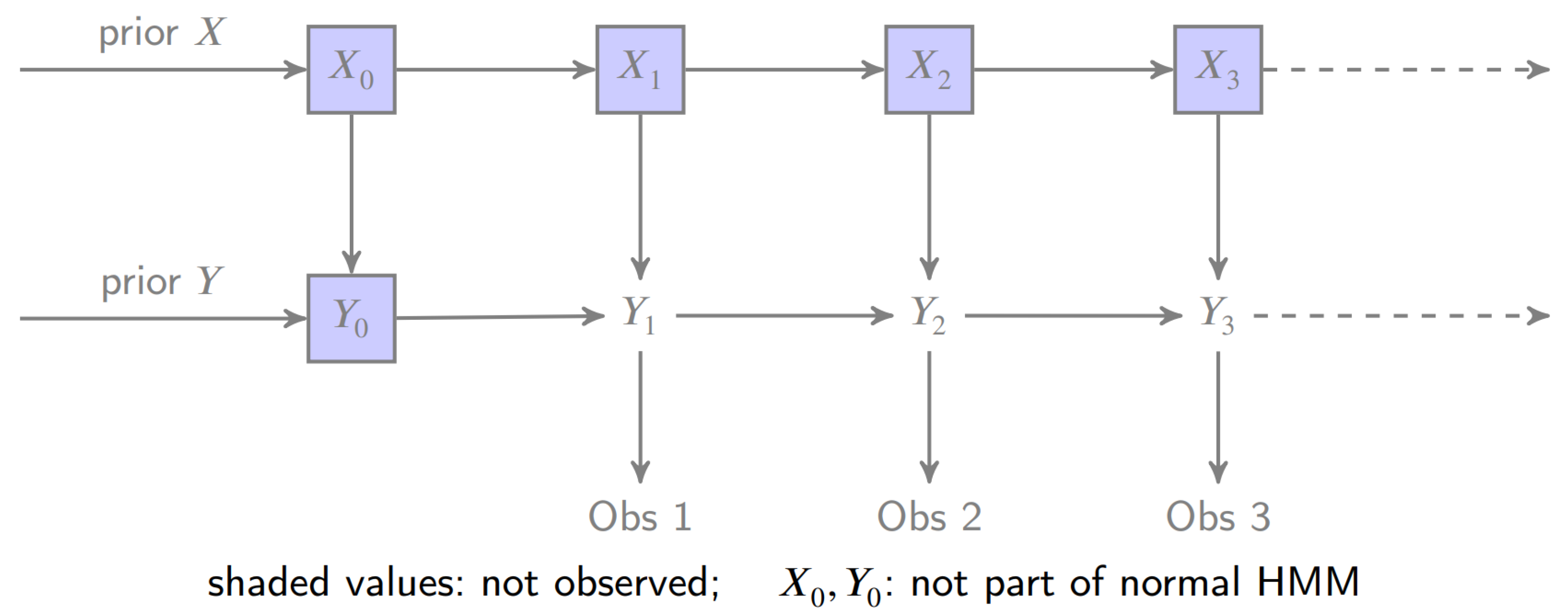
Next, we explain how MOM generalizes HMM and fits into PMC. Suppose ${\displaystyle O}$ is some discrete observation space. In MOM, like HMM, the hidden state is a homogeneous Markov chain ${\displaystyle X}$ on some discrete (finite or countable) state space ${\displaystyle E}$ with one step transition probabilities ${\displaystyle p_{x\to x^{\prime }}}$ for ${\displaystyle x,x^{\prime }\in E}$. Contrary to HMM, MOM allows self-dependence in the observations. (This is illustrated by right arrows between the Y’s in Figure 1.) In particular, MOM observations Y are a (conditional) Markov chain given the hidden state with transitions probabilities

$${\displaystyle P\left(Y_{n+1}=y|{\{X_i=x_i\}}_{i=0}^{n+1},{\{Y_j=y_j\}}_{j=0}^n\right)=q_{y_n\to y}\left(x_{n+1}\right)\forall x_0,...,x_N\in E;y,y_n\in O}$$

(3)

that do not affect the hidden state transitions in the sense

$$P(X_{n+1}=\widehat{x}|X_n=x,{\left\{X_i\right\}}_{i<n},{\left\{Y_j\right\}}_{j\le n})=p_{x\to \widehat{x}},\forall x,\widehat{x}\in E,n\in {\mathbb{N}}_0$$

(4)

still. (3) implies that

$$P\left(Y_{n+1}=y|{\left\{X_i\right\}}_{i=0}^{n+1},{\left\{Y_j\right\}}_{j\le n}\right)=P\left(Y_{n+1}=y|X_{n+1},Y_n\right),\forall y\in O$$

(5)

i.e. that the new observation only depends upon the new hidden state (as well as the past observation). (3, 4) imply that the hidden state, observation pair ${\displaystyle \left(\begin{array}{c}X\\ Y\end{array}\right)}$ is jointly Markov with joint one step transition probabilities

${\displaystyle P\left(X_{n+1}=x,Y_{n+1}=y|X_n=x_n,Y_n=y_n\right)=p_{x_n\to x}{q}_{y_n\to y}\left(x\right)\forall x,x_n\in E;y,y_n\in O.}$

The joint Markov property then implies that

${\displaystyle P\left(X_{n+1}=x,Y_{n+1}=y|X_1=x_1,Y_1=y_1,X_2=x_2,Y_2=y_2,...,X_n=x_n,Y_n=y_n\right)=p_{x_n\to x}{q}_{y_n\to y}\left(x\right).}$

Notice that this generalizes the emisson probability to

$${\displaystyle P\left(Y_n=y|X_n,X_{n-1},...,X_1;Y_{n-1},...,Y_1\right)=P\left(Y_n=y|Y_{n-1},X_n\right)=q_{Y_{n-1}\to y}\left(X_n\right)}$$

(6)

so MOM generalizes HMM by just taking $q_{Y_{n-1}\to y}\left(X_n\right)=b_{X_n}\left(y\right)$, a state dependent probability mass function. To see that MOM generalizes AR-HMM, we re-write (1) as

$$\underset{{\mathcal{Y}}_n}{\underbrace{\left[\begin{array}{c}{Y}_n\\ Y_{n-1}\\ Y_{n-2}\\ ⋮\\ Y_{n-p+1}\end{array}\right]}}=\left[\begin{array}{ccccc}{\beta }_1^{\left(X_n\right)}& {\beta }_2^{\left(X_n\right)}& {\beta }_3^{\left(X_n\right)}& \dots & {\beta }_p^{\left(X_n\right)}\\ 1& 0& 0& \dots & 0\\ 0& 1& 0& \dots & 0\\ ⋮& & \ddots & ⋮\\ 0& 0& 0& \dots 1& 0\end{array}\right]\underset{{\mathcal{Y}}_{n-1}}{\underbrace{\left[\begin{array}{c}{Y}_{n-1}\\ Y_{n-2}\\ Y_{n-3}\\ ⋮\\ Y_{n-p}\end{array}\right]}}+\left[\begin{array}{c}{\beta }_0^{\left(X_n\right)}+{\epsilon }_n\\ 0\\ 0\\ ⋮\\ 0\end{array}\right],$$

(7)

which, given the hidden state $X_n$, gives an explicit formula for ${\mathcal{Y}}_n$ in terms of only ${\mathcal{Y}}_{n-1}$ and some independent noise ${\epsilon }_n$. Hence, $\left\{{\mathcal{Y}}_n\right\}$ is obviously conditionally Markov and $\left\{(X_n,{\mathcal{Y}}_n)\right\}$ is a MOM.

A subtly that arises with MOM over HMM is that we need an enlarged initial distribution since we have a $Y_0$ that is not observed (see Figure 1). Rather, we think of starting up the observation process at time 1 even though there were observations to be had prior to this time. Further, since we generally do not know the model parameters, we need a means to estimate this initial distribution

${\displaystyle P\left(X_0\in d{x}_0,Y_0\in d{y}_0\right)=\mu \left(d{x}_0,d{y}_0\right)}$.

It is worth noting that MOM resembles the stationary PMC under Condition (H) in Pieczynski [35], which forces the Hidden state to be Markov by Proposition 2.2 of Pieczynski [35].

2.1. Simulation

Any PMC is characterized by an initial distribution $\mu$ on $E\times O$ and a joint transition probability $p_{x,y\to \widehat{x},\widehat{y}}$ for its hidden state and observations. In particular,

$$p_{x,y\to \widehat{x},\widehat{y}}=p_{x\to \widehat{x}}{q}_{y\to \widehat{y}}\left(\widehat{x}\right)$$

(8)

for MOM and

$$p_{x,y\to \widehat{x},\widehat{y}}=p_{x\to \widehat{x}}{b}_{\widehat{x}}\left(\widehat{y}\right)$$

(9)

for HMM. In any case, the marginal transitions are denoted

$$p_{x,y\to \widehat{x}}=\sum _{\widehat{y}}{p}_{x,y\to \widehat{x},\widehat{y}}\mathrm{and}{p}_{x,y\to \widehat{y}}=\sum _{\widehat{x}}{p}_{x,y\to \widehat{x},\widehat{y}}.$$

(10)

$\mu$, p characterize a $(\mu ,p)$-PMC. The initial distribution $\mu$ gives the distribution of $(X_0,Y_0)$ for MOM and PMC, while the initial distribution ${\mu }_X$ gives the distribution of $X_1$ for HMM by convention. This convention makes sense since MOM and PMC have observation history to model in some unknown $Y_0$. In the case of HMM an initial $(X_1,Y_1)$ can then be drawn from $\mu (x,y)={\mu }_X\left(x\right)b_x\left(y\right)$.

The simulation of HMM, MOM and PMC observations is done in the same way: Begin by drawing $(X_0,Y_0)$ ($(X_1,Y_1)$ for HMM) from $\mu$, continue the simulation using $p_{x,y\to \widehat{x},\widehat{y}}$ and then finally throw out the hidden state X (as well as $Y_0$ for MOM and PMC) to leave the observation process Y.

3. Likelihood, Filter and Predictor

A PMC is parameterized by its initial distribution $\mu$ and joint transition probability p for its hidden state and observations. Its ability to fit a given sequence of observations $Y_1,...,Y_n$ up to time n is naturally judged by its likelihood

$$L_n=L_n^{\mu ,p}=P(Y_1,...,Y_n)=P^{\mu ,p}(Y_1,...,Y_n)\mathrm{for}\mathrm{all}n\ge 1\mathrm{with}{L}_0=1.$$

(11)

Here $P^{\mu ,p}$ is a probability measure where ${\displaystyle \left(\begin{array}{c}X\\ Y\end{array}\right)}$ is $(\mu ,p)$-PMC. Therefore, given several $({\mu }_1,p_1),..,({\mu }_m,p_m)$ PMC models, perhaps found by different runs of an expectation-maximization algorithm, as well as an observation $Y_1,...,Y_N$ data sequence, one can use the likelihoods ${\left\{L_n^{{\mu }_i,p_i}\right\}}_{i=1}^m$ to judge which model best fits the data. Each run of the EM algorithm would converge to a local maximum of the likelihood function and then the likelihood function could be used to determine which of these produces a higher maximum. Since MOM and HMM are PMCs (with specific p given in (8), (9)), this test extends to judging best MOM and best HMM.

In applications like filtering the hidden state has significance and estimating (the distribution of) it is important. The (optimal) filter is the (conditional) hidden-state probability mass function

$${\pi }_n\left(x\right)\circeq P(X_n=x|Y_1,...,Y_n)\forall x\in E,n\ge 1.$$

(12)

We first work with the PMC and then extract MOM and HMM from these calculations. The likelihood and filter can computed together in real time using the forward probability

$$\left\{\begin{array}{ccc}{\displaystyle {\alpha }_0\left(x,y\right)}\hfill & =\hfill & P\left(Y_0=y,X_0=x\right)\hfill \\ {\alpha }_n\left(x\right)\hfill & =\hfill & P\left(Y_1,...,Y_n,X_n=x\right),1\le n\le N\hfill \end{array}\right.,$$

(13)

which is motivated from the Baum-Welch algorithm. Then, it follows from (12), (13) and (11) that

$${\pi }_n\left(x\right)={\displaystyle \frac{{\alpha }_n\left(x\right)}{{\displaystyle \sum _{\xi }}{\alpha }_n\left(\xi \right)}}={\displaystyle \frac{{\alpha }_n\left(x\right)}{L_n}}so{L}_n=\sum _{\xi }{\alpha }_n\left(\xi \right)\forall n\ge 1\mathrm{and}{\pi }_0(x,y)={\alpha }_0\left(x,y\right).$$

(14)

Moreover, we have by the joint Markov property and (13) that:

$$\begin{array}{ccc}\hfill {\displaystyle }& & {\alpha }_n\left(x\right)\hfill \\ \hfill & =& P\left(Y_1,...,Y_n,X_n=x\right)\hfill \\ \hfill & =& \sum _{x_{n-1}}P\left(Y_1,...,Y_n,X_{n-1}=x_{n-1},X_n=x\right)\hfill \\ \hfill & =& \sum _{x_{n-1}}P\left(Y_1,...,Y_{n-1},X_{n-1}=x_{n-1}\right)P(X_n=x,Y_n|Y_1,...,Y_{n-1},X_{n-1}=x_{n-1})\hfill \\ \hfill & =& \sum _{x_{n-1}}{\alpha }_{n-1}\left(x_{n-1}\right)p_{x_{n-1},Y_{n-1}\to x,Y_n},\hfill \end{array}$$

(15)

which can be solved recursively for ${\displaystyle n=2,3,...,N-1,N}$, starting at

$${\alpha }_1\left(x_1\right)=\sum _{x_0}\sum _{y_0}\mu (x_0,y_0)p_{x_0,y_0\to x_1,Y_1}.$$

(16)

Recall ${\alpha }_0=\mu$ is assigned differently. On a computer, we do not recurse ${\alpha }_n$ due to risk of underflow (the small number problem), but rather revert back to the filter ${\pi }_n$. Using (15), one finds the forward recursion for $\pi$ is:

$${\displaystyle {\rho }_n\left(x\right)=\sum _{x_{n-1}}{\pi }_{n-1}\left(x_{n-1}\right)p_{x_{n-1},Y_{n-1}\to x,Y_n},{\pi }_n\left(x\right)=\frac{{\rho }_n\left(x\right)}{a_n},a_n=\sum _{x_n}{\rho }_n\left(x_n\right),}$$

(17)

which can be solved forward for ${\displaystyle n=2,3,...,N-1,N}$, starting at

$${\displaystyle {\pi }_1\left(x\right)=\frac{\sum _{x_0}\sum _{y_0}\mu (x_0,y_0)p_{x_0,y_0\to x,Y_1}}{a_1},a_1=\sum _{x_1}\sum _{x_0}\sum _{y_0}\mu (x_0,y_0)p_{x_0,y_0\to x_1,Y_1}.}$$

(18)

This immediately implies that $L_1=a_1$ and then by using (14), (17) and induction that

$$L_n=a_1{a}_2\dots a_n⇝L_n=L_{n-1}{a}_n,L_0=1.$$

(19)

Thus, the filter and likelihood can be computed in real time (after initialization) via the recursions in (17) and (19).

Once the filter is computed, predictors can also be computed using Chapman-Kolmogorov type equations. For example, it follows by the multiplication rule and the Markov property that the one step predictor is

$$\begin{array}{ccc}\hfill P(Y_{n+1}=y_{n+1}\mid Y_1,...,Y_n)& =& \sum _{x_n,x_n+1}{\displaystyle \frac{P(Y_{n+1}=y_{n+1},X_{n+1}=x_{n+1},X_n=x_n,Y_1,...,Y_n)}{P(Y_1,...,Y_n)}}\hfill \\ \hfill & =& \sum _{x_n,x_n+1}P(Y_{n+1}=y_{n+1},X_{n+1}=x_{n+1}\mid X_n=x_n,Y_1,...,Y_n)P(X_n=x_n\mid Y_1,...,Y_n)\hfill \\ \hfill & =& \sum _{x_n,x_n+1}{p}_{x_n,Y_n\to x_{n+1},y_{n+1}}{\pi }_n\left(x_n\right),\hfill \end{array}$$

(20)

which reduces to

$$\begin{array}{c}\hfill P(Y_{n+1}=y_{n+1}\mid Y_1,...,Y_n)=\sum _{x_n,x_n+1}{p}_{x_n\to x_{n+1}}{q}_{Y_n\to y_{n+1}\left(x_{n+1}\right)}{\pi }_n\left(x_n\right),\end{array}$$

(21)

and

$$\begin{array}{c}\hfill P(Y_{n+1}=y_{n+1}\mid Y_1,...,Y_n)=\sum _{x_n,x_n+1}{p}_{x_n\to x_{n+1}}{b}_{x_{n+1}}\left(y_{n+1}\right){\pi }_n\left(x_n\right)\end{array}$$

(22)

respectively in the cases of MOM and HMM.

In non-real-time applications, we strengthen our hidden-state estimates to include future observations via the joint path filter

$${\Pi }_{n-1,n}(x,\widehat{x})=P(X_{n-1}=x,X_n=\widehat{x}\mid Y_1,...,Y_N),$$

(23)

which is a joint pmf for $n=2,...,N$. To compute the joint path filter, we first let

$$\left\{\begin{array}{ccc}{\displaystyle {\beta }_0\left(x_0,x_1,y\right)}\hfill & =\hfill & P\left(Y_1,...,Y_N|X_0=x_0,X_1=x_1,Y_0=y\right)\hfill \\ {\displaystyle {\beta }_n\left(x_n,x_{n+1}\right)}\hfill & =\hfill & P\left(Y_{n+1},...,Y_N|X_n=x_n,X_{n+1}=x_{n+1},Y_n\right),\forall 0<n<N-1\hfill \\ {\displaystyle {\beta }_{N-1}\left(x_{N-1},x_N\right)}\hfill & =\hfill & {\displaystyle P\left(Y_N|X_{N-1}=x_{N-1},X_N=x_N,Y_{N-1}\right)=\frac{p_{x_{N-1},Y_{N-1}\to x_N,Y_N}}{p_{x_{N-1},Y_{N-1}\to x_N}}}\hfill \end{array}\right.$$

(24)

and the normalized versions of $\beta$

$${\chi }_n(x,\widehat{x})={\displaystyle \frac{{\beta }_n(x,\widehat{x})}{a_{n+1}\dots a_N}},\forall n=1,...,N-1and{\chi }_0(x,\widehat{x},y)={\displaystyle \frac{{\beta }_0(x,\widehat{x},y)}{a_1\dots a_N}}.$$

(25)

(Notice we include an extra variable y in ${\alpha }_0,{\beta }_0$. This is because we do not see the first observation $Y_0$ so we have to consider all possibilities and treat it like another hidden state.) Then, by the Markov property, (19), (13) and (14)

$$\begin{array}{ccc}\hfill {\Pi }_{n-1,n}(x,\widehat{x})& =& {\displaystyle \frac{P(X_{n-1}=x,X_n=\widehat{x},Y_1,...,Y_N)}{P(Y_1,...,Y_N)}}\hfill \\ \hfill & =& {\displaystyle \frac{{\alpha }_{n-1}\left(x\right)P(X_n=\widehat{x},Y_n,...,Y_N|X_{n-1}=x,Y_1,...,Y_{n-1})}{L_N}}\hfill \\ \hfill & =& {\displaystyle \frac{{\pi }_{n-1}\left(x\right)P(X_n=\widehat{x},Y_n,...,Y_N|X_{n-1}=x,Y_{n-1})}{a_n\dots a_N}}\hfill \end{array}$$

(26)

so by (26,25,24)

$$\begin{array}{ccc}\hfill & & {\Pi }_{n-1,n}(x,\widehat{x})\hfill \\ \hfill & =& {\displaystyle \frac{{\pi }_{n-1}\left(x\right)P(X_n=\widehat{x},Y_n,...,Y_N,X_{n-1}=x,Y_{n-1})P(X_n=\widehat{x},X_{n-1}=x,Y_{n-1})}{a_n\dots a_{N}P(X_n=\widehat{x},X_{n-1}=x,Y_{n-1})P(X_{n-1}=x,Y_{n-1})}}\hfill \\ \hfill & =& {\displaystyle \frac{{\pi }_{n-1}\left(x\right)P(Y_n,...,Y_N|X_n=\widehat{x},X_{n-1}=x,Y_{n-1})P(X_n=\widehat{x}|X_{n-1}=x,Y_{n-1})}{a_n\dots a_N}}\hfill \\ \hfill & =& {\displaystyle {\pi }_{n-1}\left(x\right){\chi }_{n-1}(x,\widehat{x})p_{x,Y_{n-1}\to \widehat{x}}}\hfill \end{array}$$

(27)

for ${\displaystyle n=2,3,...,N}$. This means there are two ways to compute the (marginal) path filter directly from (27):

$${\displaystyle {\Pi }_n\left(x\right)=P(X_n=x\mid Y_1,...,Y_N)={\pi }_n\left(x\right)\sum _{x_{n+1}}{\chi }_n(x,x_{n+1})p_{x,Y_n\to x_{n+1}}}$$

(28)

for ${\displaystyle n=1,2,...,N-1}$ and

$${\displaystyle {\Pi }_n\left(x\right)=P(X_n=x\mid Y_1,...,Y_N)=\sum _{x_{n-1}}{\chi }_{n-1}\left(x_{n-1},x\right)p_{x_{n-1},Y_{n-1}\to x}{\pi }_{n-1}\left(x_{n-1}\right)}$$

(29)

for ${\displaystyle n=2,3,...,N}$. These all become computationally effective by a backward recursion for $\chi$. It also follows from (24), the Markov property and our transition probabilities that:

$$\begin{array}{ccc}\hfill {\beta }_n\left(x_n,x\right)& =& P\left(Y_{n+1},...,Y_N\mid X_n=x_n,X_{n+1}=x,Y_n\right)\hfill \\ \hfill & =& P\left(Y_{n+2},...,Y_N\mid X_n=x_n,X_{n+1}=x,Y_{n+1},Y_n\right)P\left(Y_{n+1}\mid X_n=x_n,X_{n+1}=x,Y_n\right)\hfill \\ \hfill & =& P\left(Y_{n+2},...,Y_N\mid X_{n+1}=x,Y_{n+1}\right){\displaystyle \frac{p_{x_n,Y_n\to x,Y_{n+1}}}{p_{x_n,Y_n\to x}}}\hfill \\ \hfill & =& \sum _{x^{\prime }\in E}P\left(Y_{n+2},...,Y_N\mid X_{n+2}=x^{\prime },X_{n+1}=x,Y_{n+1}\right)\hfill \\ \hfill & & *P\left(X_{n+2}=x^{\prime }\mid X_{n+1}=x,Y_{n+1}\right){\displaystyle \frac{p_{x_n,Y_n\to x,Y_{n+1}}}{p_{x_n,Y_n\to x}}}\hfill \\ \hfill & =& {\displaystyle \frac{p_{x_n,Y_n\to x,Y_{n+1}}}{p_{x_n,Y_n\to x}}}\sum _{x^{\prime }}{\beta }_{n+1}(x,x^{\prime })p_{x,Y_{n+1}\to x^{\prime }},\hfill \end{array}$$

(30)

so normalizing

$$\begin{array}{ccc}\hfill {\chi }_n\left(x_n,x\right)& =& {\displaystyle \frac{p_{x_n,Y_n\to x,Y_{n+1}}}{a_{n+1}{p}_{x_n,Y_n\to x}}}\sum _{x^{\prime }}{\chi }_{n+1}(x,x^{\prime })p_{x,Y_{n+1}\to x^{\prime }},\hfill \end{array}$$

(31)

which can be solved backward for ${\displaystyle n=N-1,N-2,...,3,2,1}$ starting from

$${\chi }_N\left(x_N,x_{N+1}\right)=1.$$

(32)

The $n=0$ value for $\pi$ and $\chi$ become

$$\begin{array}{ccc}\hfill {\chi }_0\left(x_0,x_1,y\right)& =& {\displaystyle \frac{p_{x_0,y\to x_1,Y_1}}{a_1{p}_{x_0,y\to x_1}}}\sum _{x^{\prime }}{\chi }_1(x_1,x^{\prime })p_{x_1,Y_1\to x^{\prime }},\hfill \end{array}$$

(33)

$$\begin{array}{ccc}\hfill {\pi }_0\left(x,y\right)& =& {\alpha }_0\left(x,y\right)=\mu \left(x,y\right)\hfill \end{array}$$

(34)

to account for the fact we do not see $Y_0$ as the data turns on at time 1. With ${\chi }_0$ in hand, we can estimate the joint distribution of $(X_0,Y_0)$, which are the remaining hidden variables. It follows from Bayes’ rule, (11) and (19)

$$\begin{array}{ccc}\hfill {\Pi }_0(x,y)& =& P(X_0=x,Y_0=y\mid Y_1,...,Y_N)\hfill \\ \hfill & =& {\displaystyle \frac{P(Y_1,...,Y_N\mid X_0=x,Y_0=y)P(X_0=x,Y_0=y)}{L_N}}\hfill \\ \hfill & =& {\displaystyle \frac{{\displaystyle \sum _{x_1}}P(Y_1,..,Y_N\mid X_1=x_1,X_0=x,Y_0=y)P(X_1=x_1\mid X_0=x,Y_0=y)\mu (x,y)}{a_1\dots a_N}}\hfill \\ \hfill & =& \mu (x,y)\sum _{x_1}{\chi }_0(x,x_1,y)p_{x,y\to x_1}.\hfill \end{array}$$

(35)

for all $x\in E$, $y\in O$.

The pathspace filter and likelihood algorithm is given in Algorithm 1.

Algorithm 1: Path Filter and Likelihood for PMC

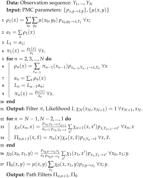The first part of Algorithm 1 up to the first set of outputs runs in real time, as the observations arrive, and provides the real-time filter and likelihood. For real time applications, one would stop there or else add predictors not included in Algorithm 1 but given as an example in (20). Otherwise, one can refine the estimates of the hidden states based upon future observations, which then provides the pathspace filters and is the key to learning a model. This is the second part of Algorithm 1 and is explained below. But first, we note that the recursions developed so far are easily tuned to MOM or HMM.

3.1. MOM Adjustments

For MOM, we use (8). We leave (13,14) and (19) unchanged so (17) and (18) become

$${\displaystyle {\rho }_n\left(x\right)=q_{Y_{n-1}\to Y_n}\left(x\right)\sum _{x_{n-1}\in E}{\pi }_{n-1}\left(x_{n-1}\right)p_{x_{n-1}\to x},{\pi }_n\left(x\right)=\frac{{\rho }_n\left(x\right)}{a_n},a_n=\sum _{x_n}{\rho }_n\left(x_n\right),}$$

(36)

for all ${\displaystyle x\in E}$, which can be solved forward for ${\displaystyle n=2,3,...,N-1,N}$, starting at

$${\displaystyle {\pi }_1\left(x\right)=\frac{{\displaystyle \sum _{x_0}}{\displaystyle \sum _{y_0}}\mu (x_0,y_0)p_{x_0\to x}{q}_{y_0\to Y_1}\left(x\right)}{a_1},a_1=\sum _{x_1}\sum _{x_0}\sum _{y_0}\mu (x_0,y_0)p_{x_0\to x_1}{q}_{y_0\to Y_1}\left(x_1\right).}$$

(37)

The backward recursions change a little more, starting with (24) and (25), which change to

$$\left\{\begin{array}{ccc}{\displaystyle {\beta }_0\left(x_1,y\right)}\hfill & =\hfill & P\left(Y_1,...,Y_N|X_1=x_1,Y_0=y\right)\hfill \\ {\displaystyle {\beta }_n\left(x_{n+1}\right)}\hfill & =\hfill & P\left(Y_{n+1},...,Y_N|X_{n+1}=x_{n+1},Y_n\right),\forall 0<n<N-1\hfill \\ {\displaystyle {\beta }_{N-1}\left(x_N\right)}\hfill & =\hfill & P\left(Y_N|X_N=x_N,Y_{N-1}\right)=q_{Y_{N-1}\to Y_N}\left(x_N\right)\hfill \end{array}\right.$$

(38)

and the normalized versions

$${\chi }_n\left(\widehat{x}\right)={\displaystyle \frac{{\beta }_n\left(\widehat{x}\right)}{a_{n+1}\dots a_N}},\forall n=1,...,N-1and{\chi }_0(\widehat{x},y)={\displaystyle \frac{{\beta }_0(\widehat{x},y)}{a_1\dots a_N}}$$

(39)

since

$$P(Y_{n+1},...,Y_N|X_n=x_n,X_{n+1}=x_{n+1},Y_n)=P(Y_n,...,Y_N|X_{n+1}=x_{n+1},Y_n)$$

(40)

by Lemma 1 (to follow). Then, (27) becomes

$$\begin{array}{c}\hfill {\displaystyle {\Pi }_{n-1,n}(x,\widehat{x})={\pi }_{n-1}\left(x\right){\chi }_{n-1}\left(\widehat{x}\right)p_{x\to \widehat{x}}}\end{array}$$

(41)

for ${\displaystyle n=2,3,...,N}$. This then implies the obvious simplifications of (28) and (29) to

$${\displaystyle {\Pi }_n\left(x\right)={\pi }_n\left(x\right)\sum _{x_{n+1}}{\chi }_n\left(x_{n+1}\right)p_{x\to x_{n+1}}and{\Pi }_n\left(x\right)={\chi }_{n-1}\left(x\right)\sum _{x_{n-1}}{p}_{x_{n-1}\to x}{\pi }_{n-1}\left(x_{n-1}\right)}$$

(42)

${\displaystyle n=1,2,...,N-1}$ and ${\displaystyle n=2,3,...,N}$ respectively. Then, (31) becomes

$$\begin{array}{ccc}\hfill {\chi }_n\left(x\right)& =& {\displaystyle \frac{q_{Y_n\to Y_{n+1}}\left(x\right)}{a_{n+1}}}\sum _{x^{\prime }}{\chi }_{n+1}\left(x^{\prime }\right)p_{x\to x^{\prime }}\hfill \end{array}$$

(43)

by (5), which is solved backwards starting from ${\chi }_N\left(x_{N+1}\right)=1$. The values at $n=0$ become

$$\begin{array}{ccc}\hfill {\chi }_0\left(x_1,y\right)& =& {\displaystyle \frac{q_{y\to Y_1}\left(x_1\right)}{a_1}}\sum _{x^{\prime }}{\chi }_1\left(x^{\prime }\right)p_{x_1\to x^{\prime }},{\pi }_0\left(x,y\right)=\mu \left(x,y\right)\hfill \end{array}$$

(44)

and

$$\begin{array}{c}\hfill {\Pi }_0(x,y)=\mu (x,y)\sum _{x_1}{\chi }_0(x_1,y)p_{x\to x_1}.\end{array}$$

(45)

for all $x\in E$, $y\in O$.

3.2. HMM Adjustments

For HMM, we use (9). We have a MOM with the specific

$$q_{y\to \widehat{y}}\left(\widehat{x}\right)=b_{\widehat{x}}\left(\widehat{y}\right)$$

(46)

that also starts at $n=1$ with $\mu (x,y)={\mu }_X\left(x\right)b_x\left(y\right)$ instead of $n=0$. This creates modest changes or simplifications for the filter startup:

$$\begin{array}{c}\hfill {\rho }_1\left(x\right)=b_x\left(Y_1\right){\mu }_X\left(x\right),a_1=\sum _x{\rho }_1\left(x\right),{\pi }_1\left(x\right)={\displaystyle \frac{{\rho }_1\left(x\right)}{a_1}}.\end{array}$$

(47)

But, otherwise (36) holds with just the substitution $q_{y\to \widehat{y}}\left(\widehat{x}\right)=b_{\widehat{x}}\left(\widehat{y}\right)$.

To handle the backward recursion, we first reduce the general definition of $\beta$ in (24) using (2) to

$$\left\{\begin{array}{ccc}{\displaystyle {\beta }_n\left(x_{n+1}\right)}\hfill & =\hfill & P\left(Y_{n+1},...,Y_N|X_{n+1}=x_{n+1}\right),\forall 0<n<N-1\hfill \\ {\displaystyle {\beta }_{N-1}\left(x_N\right)}\hfill & =\hfill & P\left(Y_N|X_N=x_N\right)=b_{x_N}\left(Y_N\right)\hfill \end{array}\right.$$

(48)

and the normalized versions

$${\chi }_n\left(x\right)={\displaystyle \frac{{\beta }_n\left(x\right)}{a_{n+1}\dots a_N}},\forall n=1,...,N-1.$$

(49)

There are no ${\alpha }_0$, ${\pi }_0$, ${\beta }_0$ nor ${\chi }_0$ variables for HMM. The HMM backward recursion simplifications are based upon the following result.

Lemma 1. 

For the MOM and HMM models

$$P\left(Y_{n+1},...,Y_N|X_n=x_n,X_{n+1}=x_{n+1},Y_n\right)=\left\{\begin{array}{cc}P\left(Y_{n+1},...,Y_N|X_{n+1}=x_{n+1},Y_n\right)\hfill & \mathrm{for}\mathrm{MOM}\hfill \\ P\left(Y_{n+1},...,Y_N|X_{n+1}=x_{n+1}\right)\hfill & \mathrm{for}\mathrm{HMM}\hfill \end{array}\right..$$

Insomuch as the proofs replicate each other we merely prove the HMM case and indicate the changes required for MOM. In the HMM case, we need only show $P\left(Y_{n+1},...,Y_N|X_n,X_{n+1},Y_n\right)$ is a function of $X_{n+1}$ only. However, it follows from the multiplication rule, the tower property and (2) that

$$\begin{array}{ccc}\hfill & & P\left(Y_{n+1},...,Y_N|X_n=x_n,X_{n+1}=x_{n+1},Y_n\right)\hfill \\ \hfill & =& {\displaystyle \frac{P\left(Y_n\mid Y_{n+1},...,Y_N,X_n=x_n,X_{n+1}=x_{n+1}\right)P\left(Y_{n+1},...,Y_N,X_n=x_n,X_{n+1}=x_{n+1}\right)}{P\left(Y_n\mid X_n=x_n,X_{n+1}=x_{n+1}\right)P\left(X_n=x_n,X_{n+1}=x_{n+1}\right)}}\hfill \\ \hfill & =& {\displaystyle \frac{P\left(Y_{n+1},...,Y_N,X_n=x_n,X_{n+1}=x_{n+1}\right)}{P\left(X_n=x_n,X_{n+1}=x_{n+1}\right)}}\hfill \\ \hfill & =& {\displaystyle \frac{{\sum }_{x_{n+2},...,x_N}P\left(X_n=x_n\right)p_{x_n\to x_{n+1}}{b}_{x_{n+1}}\left(Y_{n+1}\right)p_{x_{n+1}\to x_{n+2}}\dots p_{x_{N-1}\to x_N}{b}_{x_N}\left(Y_N\right)}{P\left(X_n=x_n\right)p_{x_n\to x_{n+1}}}}\hfill \\ \hfill & =& \sum _{x_{n+2},...,x_N}{b}_{x_{n+1}}\left(Y_{n+1}\right)p_{x_{n+1}\to x_{n+2}}{b}_{x_{n+2}}\left(Y_{n+2}\right)\dots p_{x_{N-1}\to x_N}{b}_{x_N}\left(Y_N\right),\hfill \end{array}$$

(50)

which establishes the desired dependence.

Moving to MOM, the right hand side of (50) becomes

$$\begin{array}{ccc}\hfill & & {\displaystyle \frac{P\left(Y_n,...,Y_N,X_n=x_n,X_{n+1}=x_{n+1}\right)}{P\left(Y_n,X_n=x_n,X_{n+1}=x_{n+1}\right)}}\hfill \\ \hfill & =& {\displaystyle \frac{{\sum }_{x_{n+2},...,x_N}P\left(X_n=x_n,Y_n\right)p_{x_n\to x_{n+1}}{q}_{Y_n\to Y_{n+1}}\left(x_{n+1}\right)p_{x_{n+1}\to x_{n+2}}\dots q_{Y_{N-1}\to Y_N}\left(x_N\right)p_{x_{N-1}\to x_N}}{P\left(X_n=x_n,Y_n\right)p_{x_n\to x_{n+1}}}}\hfill \\ \hfill & =& \sum _{x_{n+2},...,x_N}{q}_{Y_n\to Y_{n+1}}\left(x_{n+1}\right)p_{x_n\to x_{n+1}}\dots q_{Y_{N-1}\to Y_N}\left(x_N\right)p_{x_{N-1}\to x_N}.\square \hfill \end{array}$$

(51)

Finally, the initial probability estimate becomes

$$\begin{array}{ccc}\hfill {\displaystyle {\Pi }_1\left(x\right)}& =& P(X_1=x|Y_1,...,Y_N)\hfill \\ \hfill & =& {\displaystyle \frac{P(Y_1,...,Y_N|X_1=x)P(X_1=x)}{P(Y_1,...,Y_N)}}\hfill \\ \hfill & =& {\displaystyle \frac{{\beta }_1\left(x\right){\mu }_X\left(x\right)}{L_N}}\hfill \\ \hfill & =& {\chi }_1\left(x\right){\mu }_X\left(x\right).\hfill \end{array}$$

(52)

4. Probability Estimation via EM Algorithm

In this section, we develop a recursive expectation-maximization algorithm that can be used to create convergent estimates for the transition and initial probabilities of our models. We leave the theoretical justification of convergence to Section 6.    

Algorithm 2: EM algorithm for PMC

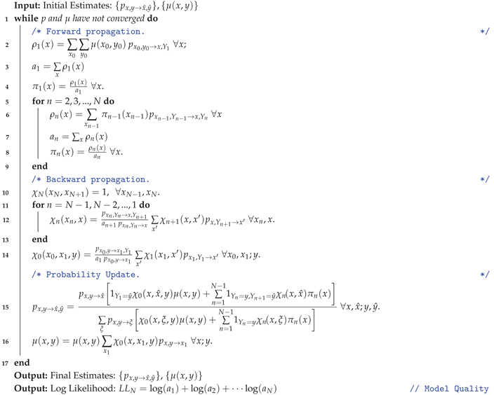    The main goal of developing an EM algorithm is to find ${\displaystyle p_{x,y\to \widehat{x},\widehat{y}}}$ for all ${\displaystyle x,\widehat{x}\in E}$, ${\displaystyle y,\widehat{y}\in O}$ and $\mu (x,y)$ for all ${\displaystyle x\in E}$, $y\in O$. Noting every time step is considered to be a transition in a discrete-time Markov chain, we would ideally set:

$$\begin{array}{ccc}& & {\displaystyle p_{x,y\to \widehat{x},\widehat{y}}=\frac{\mathrm{Expected} \mathrm{transitions}(x,y)to(\widehat{x},\widehat{y})\mathrm{given} \mathrm{observations}}{\mathrm{Expected} \mathrm{occurrences}(x,y)\mathrm{given} \mathrm{observations}}}\hfill \\ \hfill & =& {\displaystyle \frac{1_{Y_1=\widehat{y}}P(Y_0=y,X_0=x,X_1=\widehat{x}|Y_1,...,Y_N)+{\displaystyle \sum _{n=2}^N}{1}_{Y_{n-1}=y,Y_n=\widehat{y}}P(X_{n-1}=x,X_n=\widehat{x}|Y_1,...,Y_N)}{P(Y_0=y,X_0=x|Y_1,...,Y_N)+{\displaystyle \sum _{n=2}^N}{1}_{Y_{n-1}=y}P(X_{n-1}=x|Y_1,...,Y_N)}},\hfill \end{array}$$

(53)

which means we must compute ${\displaystyle P(Y_0=y,X_0=x,X_1=\widehat{x}|Y_1,...,Y_N)}$, ${\displaystyle P(Y_0=y,X_0=x|Y_1,...,Y_N)}$, and, using (23, 28), ${\displaystyle {\Pi }_n=\left(x\right)}$ for all $0\le n\le N$ and ${\displaystyle {\Pi }_{n-1,n}(x,\widehat{x})}$ for all ${\displaystyle 1\le n\le N}$ to get this transition probability estimate. Now, by Bayes’ rule, (11,19), (24,25) and (13,14)

$$\begin{array}{ccc}\hfill & & P(Y_0=y,X_0=x,X_1=\widehat{x}|Y_1,...,Y_N)\hfill \\ \hfill & =& {\displaystyle \frac{P(Y_1,...,Y_N|X_1=\widehat{x},X_0=x,Y_0=y)P(X_1=\widehat{x},X_0=x,Y_0=y)}{a_1\dots a_N}}\hfill \\ \hfill & =& {\displaystyle {\chi }_0(x,\widehat{x},y)p_{x,y\to \widehat{x}}{\pi }_0(x,y)}\hfill \end{array}$$

(54)

so

$$\begin{array}{ccc}\hfill {\Pi }_{0,1}(x,\widehat{x})& =& {\displaystyle \sum _y{\pi }_0(x,y)p_{x,y\to \widehat{x}}{\chi }_0(x,\widehat{x},y)}\hfill \end{array}$$

(55)

and so

$${\displaystyle {\Pi }_0\left(x\right)=\sum _{y,\widehat{x}}{\pi }_0(x,y)p_{x,y\to \widehat{x}}{\chi }_0(x,\widehat{x},y).}$$

(56)

${\pi }_n$ and ${\chi }_n$ are computed recursively in (17,31) using the prior estimates of ${\displaystyle p_{x,y\to \widehat{x}},\widehat{y}}$ and $\mu$.

Algorithm 3: EM algorithm for MOM

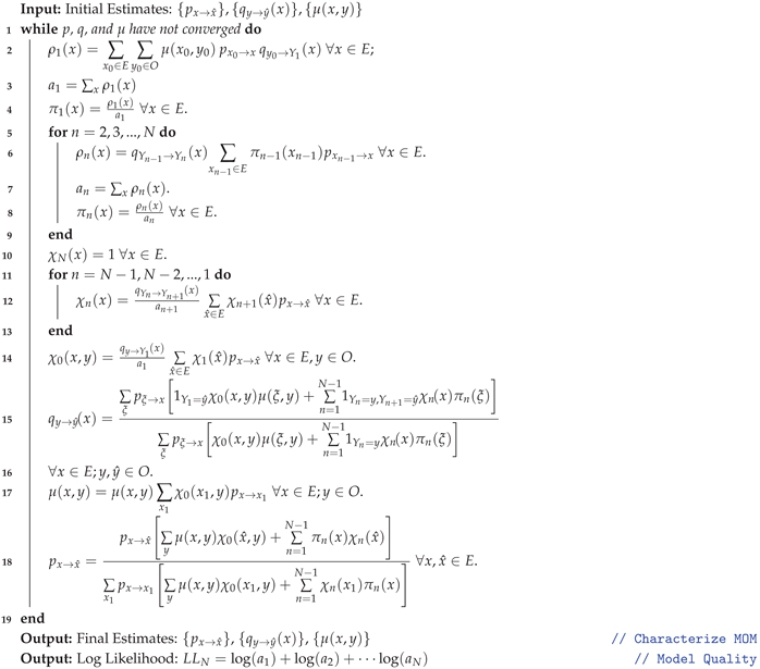Expectation-maximization algorithms use these types of formula and prior estimates to produce better estimates. We take estimates for ${\displaystyle p_{x,y\to \widehat{x},\widehat{y}}}$, and $\mu (x,y)$ and get new estimates for these quantities iteratively using (53), (54), (27), (35) and (28):

$$p_{x,y\to \widehat{x},\widehat{y}}^{\prime }={\displaystyle \frac{1_{Y_1=\widehat{y}}{\pi }_0(x,y)p_{x,y\to \widehat{x}}{\chi }_0(x,\widehat{x},y)+{\displaystyle \sum _{n=1}^{N-1}}{1}_{Y_n=y,Y_{n+1}=\widehat{y}}{\pi }_n\left(x\right)p_{x,y\to \widehat{x}}{\chi }_n(x,\widehat{x})}{{\pi }_0(x,y){\displaystyle \sum _{x_1}}{p}_{x,y\to x_1}{\chi }_0(x,x_1,y)+{\displaystyle \sum _{n=1}^{N-1}}{1}_{Y_n=y}{\pi }_n\left(x\right){\displaystyle \sum _{x_{n+1}}}{p}_{x,y\to x_{n+1}}{\chi }_n\left(x,x_{n+1}\right)}},$$

(57)

and using (35)

$$\begin{array}{ccc}\hfill {\mu }^{\prime }(x,y)& =& \sum _{x_1}{\chi }_0(x,x_1,y)p_{x,y\to x_1}\mu (x,y).\hfill \end{array}$$

(58)

Remark 1. 

1) Different iterations of $p_{x,y\to \widehat{x},\widehat{y}},\mu (x,y)$ will be used on the left and right hand sides of (57,58). The new estimates on the left are denoted $p_{x,y\to \widehat{x},\widehat{y}}^{\prime },{\mu }^{\prime }(x,y)$.

2) Setting marginal $p_{x,y\to \widehat{x}}=0$ or probability $\mu (x,y)=0$ will result in it staying zero for all updates. This effectively removes this parameter from the EM optimization update and should be avoided unless it is known that one of these should be 0.

3) If there is no successive observations with $Y_n=y$ and $Y_{n+1}=\widehat{y}$ in the actual observation sequence, then all new estimates $p_{x,y\to \widehat{x},\widehat{y}}^{\prime }$ will either be set to 0 or close to it. They might not be exactly zero due to the first term in the numerator of (57) where we could have an estimate of $Y_0=y$ and an observed $Y_1=\widehat{y}$.

We now have everything required for our EM algorithms, given for the PMC, MOM and HMM cases in Algorithms 2, 3 and 4 respectively.    

Algorithm 4: EM algorithm for HMM

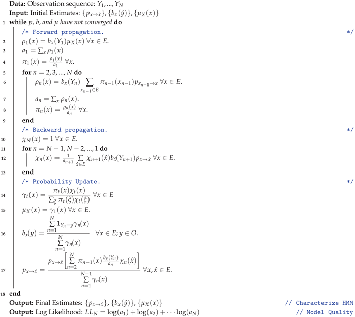These algorithms start with initial estimates $p_{x,y\to \widehat{x},\widehat{y}}^1$, ${\mu }^1(x,y)$ of $p_{x,y\to \widehat{x},\widehat{y}}$, $\mu (x,y)$; and refines them successively to new estimates $p_{x,y\to \widehat{x},\widehat{y}}^2$, ${\mu }^2(x,y)$; $p_{x,y\to \widehat{x},\widehat{y}}^3$, ${\mu }^3(x,y)$; etc. It is important to know that our estimates $\{p_{x,y\to \widehat{x},\widehat{y}}^k,{\mu }^k(x,y)\}$ improve as $k\to \infty$.

Lemma 3 (below) will be used to ensure an initially positive estimate stays positive as k increases, which is important in our proofs in Section 6. The following lemma follows easily from (31,32,33), (17,18,), induction and the fact that $\sum _{x^{\prime }}{p}_{x,Y_{n+1}\to x^{\prime }}=1$. A sensible initialization of our EM algorithm would ensure the condition $p_{x,Y_n\to \widehat{x},Y_{n+1}}>0$ holds.

Lemma 2. 

Suppose $p_{x,Y_n\to \widehat{x},Y_{n+1}}>0$ for all $x,\widehat{x}\in E$ and $n\in \{1,...,N-1\}$. Then,

• ${\chi }_m(x,\widehat{x})>0$ for all $x,\widehat{x}\in E$ and $m\in \{1,...,N-1\}$.
• ${\chi }_0(x,\widehat{x},y)>0$ for any $x,\widehat{x}\in E,y\in O$ such that $p_{x,y\to \widehat{x},Y_1}>0$.
• ${\pi }_m\left(x\right)>0$ for all $x\in E$ and $m\in \{1,...,N\}$ if in addition $\sum _{x_0,y_0}\mu (x_0,y_0)p_{x_0,y_0\to \widehat{x},Y_1}>0$ for all $\widehat{x}\in E$.
• ${\pi }_0(x,y)>0$ if $\mu (x,y)>0$.

The following result is the key to ensuring that our non-zero parameters stay non-zero. It follows from the prior lemma as well as (57,58,31).

Lemma 3. 

Suppose $N\ge 2$, $p_{x,Y_n\to \widehat{x},Y_{n+1}}>0$ for all $x,\widehat{x}\in E$ and $n\in \{1,...,N-1\}$. Then,

• $p_{x,y\to \widehat{x},\widehat{y}}^{\prime }>0$ if $p_{x,y\to \widehat{x},\widehat{y}}>0$; $\{Y_n=y,Y_{n+1}=\widehat{y}\}$ occurs; and $\sum _{x_0,y_0}\mu (x_0,y_0)p_{x_0,y_0\to x,Y_1}>0$ for all $x,x_0\in E$.
• ${\mu }^{\prime }(x,y)>0$ if $\mu (x,y)>0$ and there exists $\widehat{x}$ such that $p_{x,y\to \widehat{x},Y_1}>0$.

5. Deep Fake Application

Motivated by [27] and [4], we consider our three hidden models in deep fake generation and detection. In particular, we use the models’ EM, simulation and Bayes’ factor capabilities to generate and detect deep fake real coin flip sequences and then compare them to determine which of the three is the best at each of generation and detection.

We first created 137 real sequences of 400 coin flips by generating independent fair Bernoulli trials. Another 137 hand fake sequences of 200 coin flips were created by students with knowledge of undergraduate probability. They were told to make them look real to try to fool both humans and machines. Note that we worked with coin flip sequences of length 200 except for the training with real sequences, where 400 was used so that length was not a defining factor of these real sequence. This added length of real sequences did not bias one of the HMM, MOM or PMC over the others as it was consistent for all.

We used HMM, MOM and PMC simulation with a single hidden state variable taking s possible values (henceforth referred to as s states) to generate deep fake sequences of 200 coin flips based upon the 137 real sequences. To do this, we first learnt each of the 137 real sequences using the EM algorithms with $s+1$ hidden states for each model, creating three collections of 137 parameter sets for each s. Then, we simulated a sequence from each set of parameters throwing the hidden states away, creating three collections of 137 observation coin flip sequences for each s. These are the deep fake sequences of type HMM, MOM and PMC. Note that we learnt from the 400 long real sequences (to remove noise from the parameters) but created 200 long deep fake sequences.

Once all the five sets of (real, fake and deep fake) data was collected, we ran 100 training and testing trials at each selected s and averaged over these trials. For each trial, we randomly and independently split each of 137 (hand) fake sequences into 110 training and 27 testing sequences, i.e. an 80 to 20 split. Conversely, we re-generated the 137 independent sets of real and three deep fake sequences using respectively independent random number and Markov chain simulation with their models, but still divided these sets into 110 training and 27 testing sequences. We then trained the HMM, MOM and PMC with s hidden states on each of these sets of 110 training sequences. Note that since the deep fake sequences were generated with $s+1$ hidden states the actual model generating these sequences could not be identified. At this point, we had 110 sets of HMM parameters (i.e. HMM models) for each of the real, hand fake, HMM, MOM and PMC different training sequences in that trial. Similarly, we had 550 sets of MOM and PMC parameters.

The detection on each testing sequence was done using all the models. In a trial, each of the 5 sets of 27 sequences was run against the 550 HMM, 550 MOM and 550 PMC models. A sequence was then predicted by HMM to be real, hand fake, HMM generated, MOM generated or PMC generated based upon HMM Likelihood with s hidden states. In particular, a sequence was predicted to be real if sum of the log Likelihood over the 110 real HMM models was higher than over the 110 hand fake, 110 HMM, 110 MOM and 110 PMC HMM models. In the same way, it was predicted to be hand fake, HMM, MOM or PMC by HMM. This same procedure was repeated for MOM and for PMC and then for the remaining 99 trials, using the regeneration method mentioned above. The results were averaged and put into Tables 1, 2 and 3 in the cases $s=3,5$ and 7 respectively.

Table 1. Generative and Detection Ability with $s=3$.

	Real(%)	Handfake(%)	HMM(%)	MOM(%)	PMC(%)	Overall(%)
HMM Detection	99.96	93.36	76.89	78.25	59.79	81.65
Standard deviation	0.357	3.590	25.343	9.841	27.386	10.076
MOM Detection	99.03	89.39	98.39	91.31	77.11	91.11
Standard deviation	2.250	0.612	2.347	9.370	5.129	2.148
PMC Detection	100	70.14	95.18	90.04	88.07	88.69
Standard deviation	0.0	2.243	1.990	3.491	5.519	1.402
Overall Detection	99.66	84.30	90.15	86.53	74.99	87.15
Standard deviation	0.759	1.425	8.510	4.677	9.343	3.466

Table 1. Generative and Detection Ability with $s=3$.

	Real(%)	Handfake(%)	HMM(%)	MOM(%)	PMC(%)	Overall(%)
HMM Detection	99.96	93.36	76.89	78.25	59.79	81.65
Standard deviation	0.357	3.590	25.343	9.841	27.386	10.076
MOM Detection	99.03	89.39	98.39	91.31	77.11	91.11
Standard deviation	2.250	0.612	2.347	9.370	5.129	2.148
PMC Detection	100	70.14	95.18	90.04	88.07	88.69
Standard deviation	0.0	2.243	1.990	3.491	5.519	1.402
Overall Detection	99.66	84.30	90.15	86.53	74.99	87.15
Standard deviation	0.759	1.425	8.510	4.677	9.343	3.466

Table 2. Generative and Detection Ability with $s=5$.

	Real(%)	Handfake(%)	HMM(%)	MOM(%)	PMC(%)	Overall(%)
HMM Detection	100	94.79	73.61	64.89	63.25	79.31
Standard deviation	0	3.383	27.013	24.905	19.987	11.739
MOM Detection	98.79	89.29	95.32	87.90	79.96	90.30
Standard deviation	2.101	0.001	3.685	11.203	9.868	3.040
PMC Detection	96.71	70.82	89.54	84.18	92.32	86.71
Standard deviation	2.470	1.688	1.917	3.526	4.607	1.218
Overall Detection	98.5	84.97	86.16	78.99	78.51	85.44
Standard deviation	1.081	1.260	9.110	9.179	7.587	4.062

Table 2. Generative and Detection Ability with $s=5$.

	Real(%)	Handfake(%)	HMM(%)	MOM(%)	PMC(%)	Overall(%)
HMM Detection	100	94.79	73.61	64.89	63.25	79.31
Standard deviation	0	3.383	27.013	24.905	19.987	11.739
MOM Detection	98.79	89.29	95.32	87.90	79.96	90.30
Standard deviation	2.101	0.001	3.685	11.203	9.868	3.040
PMC Detection	96.71	70.82	89.54	84.18	92.32	86.71
Standard deviation	2.470	1.688	1.917	3.526	4.607	1.218
Overall Detection	98.5	84.97	86.16	78.99	78.51	85.44
Standard deviation	1.081	1.260	9.110	9.179	7.587	4.062

Table 3. Generative and Detection Ability with $s=7$.

	Real(%)	Handfake(%)	HMM(%)	MOM(%)	PMC(%)	Overall(%)
HMM Detection	100	95.00	41.5	55.68	33.89	65.21
Standard deviation	0	3.003	29.270	28.099	22.608	12.141
MOM Detection	98.76	89.29	96.96	90.52	90.82	93.29
Standard deviation	2.166	0.001	3.419	12.049	7.998	2.531
PMC Detection	99.82	73.25	95.75	94.21	88.32	90.27
Standard deviation	0.782	2.298	1.736	2.723	5.464	1.230
Overall Detection	99.53	85.85	78.07	80.14	71.01	82.92
Standard deviation	0.768	1.260	9.989	10.231	8.198	4.154

Table 3. Generative and Detection Ability with $s=7$.

	Real(%)	Handfake(%)	HMM(%)	MOM(%)	PMC(%)	Overall(%)
HMM Detection	100	95.00	41.5	55.68	33.89	65.21
Standard deviation	0	3.003	29.270	28.099	22.608	12.141
MOM Detection	98.76	89.29	96.96	90.52	90.82	93.29
Standard deviation	2.166	0.001	3.419	12.049	7.998	2.531
PMC Detection	99.82	73.25	95.75	94.21	88.32	90.27
Standard deviation	0.782	2.298	1.736	2.723	5.464	1.230
Overall Detection	99.53	85.85	78.07	80.14	71.01	82.92
Standard deviation	0.768	1.260	9.989	10.231	8.198	4.154

6. Convergence of Probabilities

In this section, we establish the convergence properties of the transition probabilities and initial distribution $\{p_{x,y\to \widehat{x},\widehat{y}}^k,{\mu }^k(x,y)\}$ that we derived in Section 4. Our method adapts the ideas of Baum et al. [3], Liporace [31] and Wu [45] to our setting.

We think of the transition probabilities and initial distribution as parameters, and let $\Theta$ denote all of the non-zero transition and initial distribution probabilities in $p,\mu$. Let $e=\left|E\right|$ and $o=\left|O\right|$ be the cardinalities of the hidden and observation spaces and set $d^{\prime }=e+o$. Then, $p_{x,y\to \widehat{x},\widehat{y}}:{(E\times O)}^2\to [0,1]$ has a domain space of cardinality ${\left(d^{\prime }\right)}^2$ and $\mu (x,y)\in {[0,1]}^{E\otimes O}$ has a domain space of cardinality $e\times o$. Combined this leads to ${\left(d^{\prime }\right)}^2+e\times o$ parameters. However, we are removing the values that will be set to zero and adding sum to one constraints to consider a constrained optimization problem on ${(0,\infty )}^d$ for some $d\le {\left(d^{\prime }\right)}^2+e\times o$. Removing these zero possibilities gives us necessary regularity for our re-estimation procedure. However, it was not enough to just remove them at the beginning. We had to ensure that zero parameters did not creep in during our interations or else we will be doing such things as taking logarithms of 0. Lemma 3 suggests estimates not initially set to zeros will not occur as zero in later iterations. In general, we will assume the following:

Definition 1. 

A sequence of estimates $\{p^k,q^k,{\mu }^k\}$ is zero separating if:

• $p_{x,y\to \widehat{x},\widehat{y}}^1>0$ iff $p_{x,y\to \widehat{x},\widehat{y}}^k>0$ for all $k=1,2,3,...$,
• ${\mu }^1(x,y)>0$ iff ${\mu }^k(x,y)>0$ for all $k=1,2,3,...$.

Here, iff stands for if and only if.

This means that we can potentially optimize over $p,\mu$ that we initially do not set to zero. Henceforth, we factor the zero $p,\mu$ out of $\Theta$, consider $\Theta \subset {(0,\infty )}^d$ with $d\le d^{\prime }$ and define the parameterized mass functions

$$\begin{array}{c}\hfill p_{y_0,y_1,...,y_N}(x;\Theta )=p_{x_0,y_0\to x_1,y_1}{p}_{x_1,y_1\to x_2,y_2}\dots p_{x_{N-1},y_{N-1}\to x_N,y_N}\mu (x_0,y_0)\end{array}$$

(59)

in terms of the non-zero values only. The observable likelihood

$$\begin{array}{ccc}\hfill P_{Y_1,...,Y_N}(\Theta )& =& \sum _{x_0,x_1,...,x_N}\sum _{y_0}{p}_{y_0,Y_1,...,Y_N}(x_0,x_1,...,x_N;\Theta )\hfill \end{array}$$

(60)

is not changed by removing the zero values of $p,\mu$ and this removal allows us to define the re-estimation function

$$\begin{array}{ccc}\hfill Q_{Y_1,...,Y_N}(\Theta ,{\Theta }^{\prime })& =& \sum _{x_0,...,x_N}\sum _{y_0}{p}_{y_0,Y_1,...,Y_N}(x_0,...,x_N;\Theta )ln{p}_{y_0,Y_1,...,Y_N}(x_0,...,x_N;{\Theta }^{\prime }).\hfill \end{array}$$

(61)

Note: Here and in the sequel, the summation in $P,Q$ above are only over the non-zero combinations. We would not include an $x_i,x_{i+1}$ pair where $p_{x_i,Y_j\to x_{i+1},Y_{j+1}}=0$ nor an $x_0,y_0$ pair where $\mu (x_0,y_0)=0$. Hence, our parameter space is

$$\Gamma =\{\Theta \in {(0,\infty )}^d:\sum _{\widehat{x},\widehat{y}}{p}_{x,y\to \widehat{x},\widehat{y}}=1,\sum _{x,y}\mu (x,y)=1\}.$$

Later, we will consider the extended parameter space

$$K=\{\Theta \in {[0,1]}^d:\sum _{\widehat{x},\widehat{y}}{p}_{x,y\to \widehat{x},\widehat{y}}=1,\sum _{x,y}\mu (x,y)=1\}$$

as limit points. Note: In both $\Gamma$ and K, $\Theta$ is only over the $p_{x,y\to \widehat{x},\widehat{y}}$ and $\mu (x,y)$ that are not just set to 0 (before limits).

Then, equating $Y_0$ with $y_0$ to ease notation, one has that

$$\begin{array}{ccc}\hfill Q(\Theta ,{\Theta }^{\prime })& =& \sum _{x_0,...,x_N}\sum _{y_0}\left[\prod _{n=1}^N{p}_{x_{n-1},Y_{n-1}\to x_n,Y_n}\right]\mu (x_0,y_0)\hfill \\ \hfill & & \left[\sum _{m=1}^{N}ln{p}_{x_{m-1},Y_{m-1}\to x_m,Y_m}^{\prime }+ln{\mu }^{\prime }(x_0,y_0)\right].\hfill \end{array}$$

(62)

The re-estimation function will be used to interpret the EM algorithm we derived earlier. We impose the following condition to ensure everything is well defined.

(Zero) 

The EM estimates are zero separating.

The following result is motivated by Theorem 3 of Liporace [31].

Theorem 1. 

Suppose (Zero) holds. The expectation-maximization solutions (57, 58) derived in Section 4 are theuniquecritical point of the re-estimation function ${\Theta }^{\prime }\to Q(\Theta ,{\Theta }^{\prime })$, subject to ${\Theta }^{\prime }$ forming probability mass functions. This critical point is a maximum taking value in ${(0,1]}^d$ for d explained above.

We consider it as an optimization problem over the open set ${(0,\infty )}^d$ but with the constraint that we have mass functions so the values have to be in the set ${(0,1]}^d$.

One has by (62) as well as the constraint ${\sum }_{\widehat{x},\widehat{y}}{p}_{x,y\to \widehat{x},\widehat{y}}^{\prime }=1$ that the maximum must satisfy

$$\begin{array}{ccc}\hfill 0& =& {\displaystyle \frac{\partial }{\partial p_{x,y\to \widehat{x},\widehat{y}}^{\prime }}}\left\{Q(\Theta ,{\Theta }^{\prime })-\lambda \left(\sum _{\xi ,\theta }{p}_{x,y\to \xi ,\theta }^{\prime }-1\right)\right\}\hfill \\ \hfill & =& \sum _{x_0,...,x_N}\sum _{y_0}\left[\prod _{n=1}^N{p}_{x_{n-1},Y_{n-1}\to x_n,Y_n}\right]\sum _{m=1}^N{\displaystyle \frac{1_{x_{m-1}=x,Y_{m-1}=y}{1}_{x_m=\widehat{x},Y_m=\widehat{y}}}{p_{x,y\to \widehat{x},\widehat{y}}^{\prime }}}\mu (x_0,y_0)-\lambda \hfill \end{array}$$

(63)

where $\lambda$ is a Lagrange multiplier and $Y_{m-1}=y$ means $Y_0=y_0$ when $m=1$. Multiplying by $p_{x,y\to \widehat{x},\widehat{y}}^{\prime }$, summing over $\widehat{x},\widehat{y}$ and then using (11, 35, 28) and then (19,14,25) one has that

$$\begin{array}{ccc}\hfill \lambda & =& \sum _{m=1}^N\sum _{x_0,...,x_N}\sum _{y_0}\left[\prod _{n=1}^N{p}_{x_{n-1},Y_{n-1}\to x_n,Y_n}\right]1_{x_{m-1}=x,Y_{m-1}=y}\mu (x_0,y_0)\hfill \\ \hfill & =& P(X_0=x,Y_0=y,Y_1,...,Y_N)+\sum _{m=2}^N{1}_{Y_{m-1}=y}P(X_{m-1}=x,Y_1,...,Y_N)\hfill \\ \hfill & =& {\Pi }_0(x,y)L_N+\sum _{m=2}^N{1}_{Y_{m-1}=y}{\Pi }_{m-1}\left(x\right)L_N\hfill \\ \hfill & =& \sum _{x_1}{\beta }_0(x,x_1,y)p_{x,y\to x_1}{\alpha }_0(x,y)+\sum _{m=2}^N\sum _{x_m}{1}_{Y_{m-1}=y}{\beta }_{m-1}(x,x_m)p_{x,Y_{m-1}\to x_m}{\alpha }_{m-1}\left(x\right).\hfill \end{array}$$

(64)

Substituting (64) into (63) and repeating the argument in (64) but with (27) instead of (28), one has that

$$\begin{array}{ccc}\hfill {\displaystyle p_{x,y\to \widehat{x},\widehat{y}}^{\prime }}& =& \sum _{x_0,...,x_N}\sum _{y_0}\left[\prod _{n=1}^N{p}_{x_{n-1},Y_{n-1}\to x_n,Y_n}\right]\sum _{m=1}^N{\displaystyle \frac{1_{x_{m-1}=x,Y_{m-1}=y,x_m=\widehat{x},Y_m=\widehat{y}}}{\lambda }}\mu (x_0,y_0)\hfill \\ \hfill & =& {\displaystyle \frac{1_{Y_1=\widehat{y}}P(X_0=x,Y_0=y,X_1=\widehat{x},Y_1,...,Y_N)+{\displaystyle \sum _{m=2}^N}{1}_{Y_{m-1}=y,Y_m=\widehat{y}}P(X_{m-1}=x,X_m=\widehat{x},Y_1,...,Y_N)}{{\displaystyle \sum _{x_1}}{\beta }_0(x,x_1,y)p_{x,y\to x_1}{\alpha }_0(x,y)+{\displaystyle \sum _{m=2}^N}{\displaystyle \sum _{x_m}}{1}_{Y_{m-1}=y}{\beta }_{m-1}(x,x_m)p_{x,Y_{m-1}\to x_m}{\alpha }_{m-1}\left(x\right)}}\hfill \\ \hfill & =& {\displaystyle \frac{1_{Y_1=\widehat{y}}{\chi }_0(x,\widehat{x},y)p_{x,y\to \widehat{x}}{\pi }_0(x,y)+{\displaystyle \sum _{m=2}^N}{1}_{Y_{m-1}=y,Y_m=\widehat{y}}{\chi }_{m-1}(x,\widehat{x})p_{x,Y_{m-1}\to \widehat{x}}{\pi }_{m-1}\left(x\right)}{{\displaystyle \sum _{x_1}}{\chi }_0(x,x_1,y)p_{x,y\to x_1}{\pi }_0(x,y)+{\displaystyle \sum _{m=2}^N}{\displaystyle \sum _{x_m}}{1}_{Y_{m-1}=y}{\chi }_{m-1}(x,x_m)p_{x,Y_{m-1}\to x_m}{\pi }_{m-1}\left(x\right)}}.\hfill \end{array}$$

(65)

To explain the first term in the numerator in the last equality, we use multiplication rule and (24) to find

$$P(X_0=x,Y_0=y,X_1=\widehat{x},Y_1,...,Y_N)={\beta }_0(x,\widehat{x},y)P(X_0=x,Y_0=y,X_1=\widehat{x})={\chi }_0(x,\widehat{x},y)L_N{\pi }_0(x,y)p_{x,y\to \widehat{x}}$$

from which it will follow easily.

Finally, for a maximum one also requires

$$\begin{array}{ccc}\hfill 0& =& {\displaystyle \frac{\partial }{\partial {\mu }^{\prime }(x,y)}}\left\{Q(\Theta ,{\Theta }^{\prime })-\lambda \left(\sum _{\xi \in E,\theta \in O}{\mu }^{\prime }(\xi ,\theta )-1\right)\right\}\hfill \\ \hfill & =& \sum _{x_0,...,x_N}\sum _{y_0}\left[\prod _{n=1}^N{p}_{x_{n-1},Y_{n-1}\to x_n,Y_n}\right]{\displaystyle \frac{1_{x_0=x}{1}_{y_0=y}}{{\mu }^{\prime }(x,y)}}\mu (x_0,y_0)-\lambda ,\hfill \end{array}$$

(66)

where $\lambda$ is a Lagrange multiplier. Multiplying by ${\mu }^{\prime }(x,y)$ and summing over $x,y$, one has that

$$\begin{array}{ccc}\hfill \lambda & =& \sum _{x_0,...,x_N}\sum _{y_0}\left[\prod _{n=1}^N{p}_{x_{n-1},Y_{n-1}\to x_n,Y_n}\right]\mu (x_0,y_0)\hfill \\ \hfill & =& P(Y_1,...,Y_N)\hfill \\ \hfill & =& L_N.\hfill \end{array}$$

(67)

Substituting (67) into (66), one has by (35) that

$$\begin{array}{ccc}\hfill {\displaystyle {\mu }^{\prime }(x,y)}& =& {\displaystyle \frac{\sum _{x_0,...,x_N}\sum _{y_0}\left[\prod _{n=1}^N{p}_{x_{n-1},Y_{n-1}\to x_n,Y_n}\right]1_{x_0=x}{1}_{y_0=y}\mu (x_0,y_0)}{L_N}}\hfill \\ \hfill & =& {\displaystyle \frac{P(X_0=x,Y_0=y,Y_1,...,Y_N)}{L_N}}\hfill \\ \hfill & =& {\pi }_0(x,y)\sum _{x_1}{\chi }_0(x,x_1,y)p_{x,y\to x_1}.\hfill \end{array}$$

(68)

Now, we have established that the EM algorithm of Section 4 corresponds to the unique critical point of ${\Theta }^{\prime }\to Q(\Theta ,{\Theta }^{\prime })$. Moreover, all mixed partial derivative of Q in the components of ${\Theta }^{\prime }$ are 0, while

$$\begin{array}{ccc}& & {\displaystyle \frac{{\partial }^2{Q}_{Y_1,Y_2,...,Y_N}(\Theta ,{\Theta }^{\prime })}{{\partial p_{x,y\to \widehat{x},\widehat{y}}^{\prime }}^2}}\hfill \\ \hfill & =& -\sum _{y_0;x_0,...,x_N}\left[\prod _{n=1}^N{p}_{x_{n-1},Y_{n-1}\to x_n,Y_n}\right]\sum _{m=1}^N{\displaystyle \frac{1_{X_{m-1}=x,Y_{m-1}=y,x_m=\widehat{x},Y_m=\widehat{y}}}{{p_{x,y\to \widehat{x},\widehat{y}}^{\prime }}^2}}\mu (x_0,y_0)\hfill \end{array}$$

(69)

and

$$\begin{array}{ccc}& & {\displaystyle \frac{{\partial }^2{Q}_{Y_1,Y_2,...,Y_N}(\Theta ,{\Theta }^{\prime })}{{\partial {\mu }^{\prime }(x,y)}^2}}\hfill \\ \hfill & =& -\sum _{y_0;x_0,...,x_N}\left[\prod _{n=1}^N{p}_{x_{n-1},Y_{n-1}\to x_n,Y_n}\right]\sum _{m=1}^N{\displaystyle \frac{1_{y_0=y,x_0=x}}{{{\mu }^{\prime }(x,y)}^2}}\mu (x_0,y_0).\hfill \end{array}$$

(70)

Hence, the Hessian matrix is diagonal with negative values along its axis and the critical point is a maximum.

The upshot of this result is that, if the EM algorithm produces parameters $\left\{{\Theta }^k\right\}\subset \Gamma$, then $Q({\Theta }^k,{\Theta }^{k+1})\ge Q({\Theta }^k,{\Theta }^k)$.

Now, we have the following result, based upon Theorem 2.1 of Baum et al. [3], that establishes the observable likelihood is also increasing i.e. $P\left({\Theta }^{k+1}\right)\ge P\left({\Theta }^k\right)$.

Lemma 4. 

Suppose (Zero) holds. $Q(\Theta ,{\Theta }^{\prime })\ge Q(\Theta ,\Theta )$ implies $P\left({\Theta }^{\prime }\right)\ge P(\Theta )$. Moreover, $Q(\Theta ,{\Theta }^{\prime })>Q(\Theta ,\Theta )$ implies $P\left({\Theta }^{\prime }\right)>P(\Theta )$.

$ln\left(t\right)$ for $t>0$ has convex inverse $exp\left(t\right)$. Hence, by Jensen’s inequality

$$\begin{array}{ccc}\hfill {\displaystyle }& & {\displaystyle \frac{Q(\Theta ,{\Theta }^{\prime })-Q(\Theta ,\Theta )}{P(\Theta )}}\hfill \\ \hfill & =& lnexp\left[\sum _{x_0,x_1,...,x_N}\sum _{y_0}ln\left({\displaystyle \frac{p_{y_0,Y_1,...,Y_N}(x_0,x_1,...,x_N;{\Theta }^{\prime })}{p_{y_0,Y_1,...,Y_N}(x_0,x_1,...,x_N;\Theta )}}\right){\displaystyle \frac{p_{y_0,Y_1,...,Y_N}(x_0,x_1,...,x_N;\Theta )}{P(\Theta )}}\right]\hfill \\ \hfill & \le & ln\left({\displaystyle \frac{{\displaystyle \sum _{x_0,x_1,...,x_N}}{\displaystyle \sum _{y_0}}{p}_{y_0,Y_1,...,Y_N}(x_0,x_1,...,x_N;\Theta )\frac{p_{y_0,Y_1,...,Y_N}(x_0,x_1,...,x_N;{\Theta }^{\prime })}{p_{y_0,Y_1,...,Y_N}(x_0,x_1,...,x_N;\Theta )}}{P(\Theta )}}\right)\hfill \\ \hfill & =& ln\left({\displaystyle \frac{P\left({\Theta }^{\prime }\right)}{P(\Theta )}}\right)\hfill \end{array}$$

(71)

and the result follows.

The stationary points of P and Q are also related.

Lemma 5. 

Suppose (Zero) holds. A point $\Theta \in \Gamma$ is a critical point of $P(\Theta )$ if and only if it is a fixed point of the re-estimation function, i.e. $Q(\Theta ;\Theta )={max}_{{\Theta }^{\prime }}Q(\Theta ;{\Theta }^{\prime })$ since Q is differentiable on ${(0,\infty )}^d$ in ${\Theta }^{\prime }$.

The following derivatives are equal:

$$\begin{array}{ccc}\hfill {\displaystyle \frac{\partial P_{Y_1,...,Y_N}(\Theta )}{\partial p_{x,y\to \widehat{x},\widehat{y}}}}& =& \sum _{x_0,...,x_N}\sum _{y_0}\left[\prod _{n=1}^N{p}_{x_{n-1},Y_{n-1}\to x_n,Y_n}\right]\sum _{m=1}^N{\displaystyle \frac{1_{x_{m-1}=x,Y_{m-1}=y,x_m=\widehat{x},Y_m=\widehat{y}}}{p_{x_{m-1}\to x_m}}}\mu (x_0,y_0)\hfill \\ \hfill & =& {\displaystyle \frac{\partial Q_{Y_1,Y_2,...,Y_N}(\Theta ,{\Theta }^{\prime })}{p_{x,y\to \widehat{x},\widehat{y}}}}{|}_{{\Theta }^{\prime }=\Theta },\hfill \end{array}$$

(72)

which are defined since $p_{x,y\to \widehat{x},\widehat{y}}\ne 0$. Similarly,

$$\begin{array}{ccc}\hfill {\displaystyle \frac{\partial P_{Y_1,...,Y_N}(\Theta )}{\partial \mu (x,y)}}& =& \sum _{x_0,...,x_N}\sum _{y_0}\left[\prod _{n=1}^N{p}_{x_{n-1},Y_{n-1}\to x_n,Y_n}\right]1_{(x_0,y_0)=(x,y)}\hfill \\ \hfill & =& {\displaystyle \frac{\partial Q_{Y_1,Y_2,...,Y_N}(\Theta ,{\Theta }^{\prime })}{\partial {\mu }^{\prime }(x,y)}}{|}_{{\Theta }^{\prime }=\Theta }.\hfill \end{array}$$

(73)

We can rewrite (65,68) in recursive form with the values of $\pi$ and $\chi$ substituted in to find that

$${\Theta }^{k+1}=M\left({\Theta }^k\right),$$

where M is a continuous function. Moreover, $P:K\to [0,1]$ is continuous and satisfies $P\left({\Theta }^k\right)\le P\left(M\left({\Theta }^k\right)\right)$ from above. Now, we have established everything we need for the following result, which follows from the proof of Theorem 1 of Wu [45].

Theorem 2. 

Suppose (Zero) holds. Then, ${\left\{{\Theta }^k\right\}}_{k=1}^{\infty }$ is relatively compact, all its limit points (in K) are stationary points of P, producing the same likelihood $P\left({\Theta }^{*}\right)$ say, and $P\left({\Theta }^k\right)$ converges monotonically to $P\left({\Theta }^{*}\right)$.

Wu [45] has several interesting results in the context of general EM algorithms to guarantee convergence to local or global maxima under certain conditions. However, the point of this note is to introduce a new model and algorithms with just enough theory to justify the algorithms. Hence, we do not consider theory under any special cases here but rather refer the reader to Wu [45].

References

- L. E. Baum and T. Petrie. Statistical Inference for Probabilistic Functions of Finite State Markov Chains. The Annals of Mathematical Statistics. 37 (6): 1554-1563, 1966. [CrossRef]
- L. E. Baum and J. A. Eagon. An inequality with applications to statistical estimation for probabilistic functions of Markov processes and to a model for ecology. Bulletin of the American Mathematical Society. 73 (3): 360, 1967. [CrossRef]
- L. E. Baum, T. Petrie, G. Soules and N. Weiss. A Maximization Technique Occurring in Statistical Analysis of Probabilistic Functions in Markov Chains. The Annals of Mathematical Statistics, 41, 164-171, 1970. [CrossRef]
- J. Bhadana, M. A. Kouritzin, S. Park and I. Zhang. Markov Processes for Enhanced Deepfake Generation and Detection. arXiv 2411.07993 (2024). [CrossRef]
- P. Bonate Pharmacokinetic-Pharmacodynamic Modeling and Simulation. Berlin: Springer, 2011.
- J. D. Bryan and S. E. Levinson. Autoregressive Hidden Markov Model and the Speech Signal. Procedia Computer Science 61 328-333, 2015.
- O. Cappé, E. Moulines and T. Rydén. Inference in Hidden Markov Models. Springer, Berlin 2007.
- N. Chopin. Central Limit Theorem for Sequential Monte Carlo Methods and its Application to Bayesian Inference. The Annals of Statistics 32 (6), 2385–2411, 2004.
- N. Chopin and O. Papaspiliopoulos. An Introduction to Sequential Monte Carlo. Springer Nature, Switzerland AG 2020. [CrossRef]
- D. Creal. A Survey of Sequential Monte Carlo Methods for Economics and Finance. Econometric Reviews. 31 (2), 2012. [CrossRef]
- D. Crisan, M. A. Kouritzin and J. Xiong. Nonlinear filtering with signal dependent observation noise. Electronic Journal of Probability, 14 1863-1883, 2009. [CrossRef]
- E. D’Amato, I. Notaro, V. A. Nardi, and V. Scordamaglia. A Particle Filtering Approach for Fault Detection and Isolation of UAV IMU Sensors: Design, Implementation and Sensitivity Analysis. Sensors. 21 (9), 2021. [CrossRef]
- P. Date, R. Mamon and A. Tenyakov. Filtering and forecasting commodity futures prices under an HMM framework. Energy Economics, 40, 1001-1013, 2013. [CrossRef]
- P. Del Moral, M. A. Kouritzin and L. Miclo. On a class of discrete generation interacting particle systems. Electronic Journal of Probability 6 : Paper No. 16, 26 p., 2001.
- S. Derrode and W. Pieczynski. Unsupervised data classification using pairwise Markov chains with automatic copula selection. Computational statistics and data analysis 63: 81-98, 2013.
- S. Derrode and W. Pieczynski. Unsupervised classification using hidden Markov chain with unknown noise copulas and margins. Signal Processing 128: 8-17, 2016.
- J. Elfring, E. Torta and R. van de Molengraft. Particle Filters: A Hands-On Tutorial. Sensors (Basel) 21 (2):438, 2021. [CrossRef]
- M. Fujisaki, G. Kallianpur and H. Kunita. Stochastic differential equations for the nonlinear filtering problem. Osaka J. Math. 9, 19–40, 1972.
- E. Hajiramezanali, M. Imani, U. Braga-Neto, X. Qian and E. R. Dougherty. Scalable optimal Bayesian classification of single-cell trajectories under regulatory model uncertainty. BMC Genomics 20 (Suppl 6): 435, 2019. [CrossRef]
- R. E. Kalman. A New Approach to Linear Filtering and Prediction Problems. Journal of Basic Engineering. 82: 35-45, 1960. [CrossRef]
- R. E. Kalman and R. S. Bucy. New Results in Linear Filtering and Prediction Theory. ASME. J. Basic Eng. 83(1): 95-108, 1961. [CrossRef]
- T. Kloek and H. K. van Dijk. Bayesian Estimates of Equation System Parameters: An Application of Integration by Monte Carlo. Econometrica. 46 (1): 1-19, 1978. [CrossRef]
- M. A. Kouritzin. On exact filters for continuous signals with discrete observations, IEEE Transactions on Automatic Control, vol. 43, no. 5, pp. 709-715, 1998. [CrossRef]
- M. A. Kouritzin. Residual and Stratified Branching Particle Filters. Computational Statistics and Data Analysis 111, pp. 145-165, 2017. [CrossRef]
- M. A. Kouritzin. Sampling and filtering with Markov chains. Signal Processing 2251, ISSN 0165-1684, 2024. [CrossRef]
- M. A. Kouritzin and H. Long. On extending classical filtering equations. Statistics and Probability Letters. 78 3195-3202, 2008. [CrossRef]
- M.A. Kouritzin, F. Newton, S. Orsten, D.C. Wilson. On Detecting Fake Coin Flip Sequences, IMS Collections 4 Markov Processes and Related Topics: A Festschrift for Thomas G. Kurtz, pp. 107-122, 2008.
- K. Kuljus and J. Lember. Pairwise Markov Models and Hybrid Segmentation Approach. Methodol Comput Appl Probab 25, 67, 2023. [CrossRef]
- T. G. Kurtz and D. L. Ocone. Unique characterization of conditional distributions in nonlinear filtering. Ann. Probab. 16, 80–107, (1988).
- T. G. Kurtz, and G. Nappo. The Filtered Martingale Problem. in The Oxford Handbook of Nonlinear Filtering, Oxford University Press, 2010.
- L. A. Liporace. Maximum likelihood estimation for multivariate observations of Markov sources. IEEE Trans. Inf. Theory 28(5): 729-734, (1982).
- V. Maroulas and A. Nebenführ. Tracking Rapid Intracellular Movements: A Bayesian Random Set Approach. The Annals of Applied Statistics 9 (2): 926-949, 2015. [CrossRef]
- C. Nicolai. Solving ion channel kinetics with the QuB software. Biophysical Reviews and Letters 8 (3n04): 191-211, 2013 ). [CrossRef]
- A. Petropoulos, S. P. Chatzis and S. Xanthopoulos. A novel corporate credit rating system based on Student’s-t hidden Markov models. Expert Systems with Applications. 53: 87-105, 2016. [CrossRef]
- W. Pieczynski. Pairwise Markov chains. IEEE Transactions on Pattern Analysis and Machine Intelligence, 25 (5), 634-639, (2003). [CrossRef]
- M. K. Pitt and N. Shephard. Filtering Via Simulation: Auxiliary Particle Filters. Journal of the American Statistical Association. 94 (446): 590-591, (1999). [CrossRef]
- L. R. Rabiner. A tutorial on hidden Markov models and selected applications in speech recognition. Proceedings of the IEEE 77 (2): 257–286,1989. CiteSeerX 10.1.1.381.3454. [CrossRef]
- R. Shinghal and G. T. Toussaint. Experiments in text recognition with the modified Viterbi algorithm. IEEE Transactions on Pattern Analysis and Machine Intelligence, PAMI-l 184-193, 1979.
- E. Sidrow, N. Heckman, S. M. Fortune, A. W. Trites, I. Murphy and M. Auger-Méthé. Modelling multi-scale, state-switching functional data with hidden Markov models. Canadian Journal of Statistics, 50(1), 327-356, (2022).
- I. Stanculescu, C. K. I. Williams and Y. Freer. Autoregressive Hidden Markov Models for the Early Detection of Neonatal Sepsis. IEEE Journal of Biomedical and Health Informatics 18(5):1560-1570, 2014. DOI: 10.1109/JBHI.2013.2294692.
- J. Stigler, F. Ziegler, A. Gieseke, J. C. M. Gebhardt and M. Rief. The Complex Folding Network of Single Calmodulin Molecules. Science. 334 (6055): 512-516, 2011. Bibcode:2011Sci...334..512S. [CrossRef]
- H. K. van Dijk and T. Kloek. Experiments with some alternatives for simple importance sampling in Monte Carlo integration. In Bernardo, J. M.; DeGroot, M. H.; Lindley, D. V.; Smith, A. F. M. (eds.). Bayesian Statistics. Vol. II. Amsterdam: North Holland, 1984. ISBN 0-444-87746-0.
- P. J. Van Leeuwen, H. R. Künsch, L. Nerger, R. Potthast and S. Reich. Particle filters for high-dimensional geoscience applications: A review. Q. J. R. Meteorol Soc. 145: 2335–2365, 2019. [CrossRef]
- A. J. Viterbi. Error bounds for convolutional codes and an asymptotically optimum decoding algorithm. IEEE Transactions on Information Theory. 13 (2): 260-269, 1967. [CrossRef]
- C. F. J. Wu. On the Convergence Properties of the EM Algorithm, Ann. Statist. 11(1): 95-103, 1983.
- T. Xuan. Autoregressive Hidden Markov Model with Application in an El Nino Study. MSc. Thesis, University of Saskatchewan, Saskatoon, 2004.
- M. Zakai. On the optimal filtering of diffusion processes. Z. Wahrsch. Verw. Gebiete 11, 230–243, (1969).
Figure 1.
Markov Observation Model Structure.
Disclaimer/Publisher’s Note: The statements, opinions and data contained in all publications are solely those of the individual author(s) and contributor(s) and not of MDPI and/or the editor(s). MDPI and/or the editor(s) disclaim responsibility for any injury to people or property resulting from any ideas, methods, instructions or products referred to in the content. |
© 2025 by the authors. Licensee MDPI, Basel, Switzerland. This article is an open access article distributed under the terms and conditions of the Creative Commons Attribution (CC BY) license (http://creativecommons.org/licenses/by/4.0/).
Copyright: This open access article is published under a Creative Commons CC BY 4.0 license, which permit the free download, distribution, and reuse, provided that the author and preprint are cited in any reuse.