
Submitted:
01 June 2025
Posted:
02 June 2025
You are already at the latest version
Abstract
We will show that we can model the Planck´s length expansion (1.28 10⁻⁵⁴ m < Lpɢ < 1.61 10⁻³⁵ m) as a function of the redshift z. Recall that in the theory: RLC electrical model of a black hole and the early universe, we proposed that when a black hole forms the Planck´s length corresponds to Lpɛ = 1.61 10⁻³⁵ m; as the black hole grows, the Planck´s length decreases until the black hole reaches its critical mass and then disintegrates, at which point the Planck´s length reaches the value of Lpɢ = 1.28 10⁻⁵⁴ m. This will allow us to understand dark energy and the Hubble´s tension problem, that is, the discrepancy with the Hubble´s constant.
Keywords:
RLC electrical model
; RC electrical model
; cosmology
; astronomy
; astrophysics
; background radiation
; Hubble’s law
; Boltzmann´s constant
; dark energy
; dark matter
; black hole
; Big Bang
; cosmic inflation
; early universe
; quantum gravity
; CERN
; LHC
; Fermilab
; general relativity
; particle physics
; condensed matter physics
; M theory
; super string theory
; extra dimensions
1. Cosmological Redshift Theory
Cosmological redshift is a fundamental concept in astrophysics and cosmology that describes the stretching of light waves as they travel through an expanding universe. It occurs due to the large-scale expansion of space itself, rather than the motion of individual astronomical objects.
Cosmological redshift is a key phenomenon in astrophysics and cosmology, associated with the expansion of the universe. It manifests itself as a red-shift in the electromagnetic spectrum of light coming from distant objects. The magnitude of this shift is directly related to the scale factor of the universe and provides crucial information about cosmic evolution.
1.1. Understanding Redshift
Redshift refers to the increase in the wavelength of electromagnetic radiation, shifting visible light towards the red end of the spectrum. It is mathematically expressed using the equation:
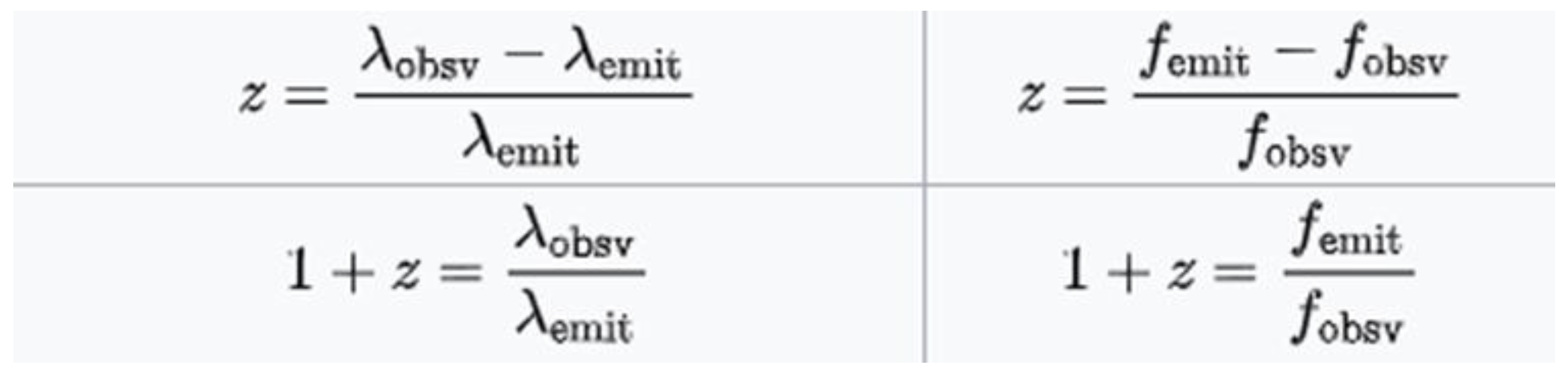
Figure 1.
Redshift equation.
Where (λobsv) represents the wavelength measured by the observer and ( λemit ) the wavelength at the time of emission.
The cosmological redshift is directly linked to the scale factor of the universe. It is described by Hubble’s Law:
v = H0 x d
Where v is the recession velocity of a galaxy, H0 is Hubble’s constant, and d is the distance to the galaxy. This relationship demonstrates that galaxies farther from us recede at greater velocities, implying an expanding universe.
Implications for Cosmology
Cosmological redshift helps scientists:
- Determine the age and expansion rate of the universe.
- Measure distances to faraway galaxies.
- Understand the evolution of cosmic structures.
1.2. Types of Redshifts
There are three primary causes of redshift:
- Doppler Redshift: Due to the relative motion of objects moving away from an observer.
- Gravitational Redshift: Caused by light escaping a strong gravitational field.
- Cosmological Redshift: Resulting from the expansion of the universe itself, affecting all wavelengths of light traveling over vast cosmic distances.
2. Application of the Model and Results
2.1. Observations in Astronomy
The redshift observed in astronomy can be measured because the emission and absorption spectra for atoms are distinctive and well known, calibrated from spectroscopic experiments in laboratories on Earth. When the redshifts of various absorption and emission lines from a single astronomical object are measured, z is found to be remarkably constant. Although distant objects may be slightly blurred and lines broadened, it is by no more than can be explained by thermal or mechanical motion of the source.
Determining the redshift of an object with spectroscopy requires the wavelength of the emitted light in the rest frame of the source. Astronomical applications rely on distinct spectral lines. Redshifts cannot be calculated by looking at unidentified features whose rest-frame frequency is unknown, or with a spectrum that is featureless or white noise (random fluctuations in a spectrum). Thus gamma-ray bursts themselves cannot be used for reliable redshift measurements, but optical afterglow associated with the burst can be analysed for redshifts.
2.2. RC Electrical Modelling of the Cosmological Redshift (z)
To model the cosmological redshift, we will use the charge model of an RC circuit which we will represent below:
Figure 3 represents the charge of a capacitor, which can be described by the following equation:
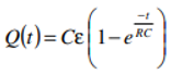
Let's analyse equation (1):
T → 0, Q(t) → 0
T → 5RC, Q(t) → Cɛ
Using equation (1), we are going to model the graph in Figure 2, for this we are going to propose the following graph:
For the model represented by the blue line, equation (1) can be written as follows:
We observe that the model represented by the blue line, the constant Tau, τ = RC = 2.
For the model represented by the green line, equation (1) can be written as follows:
We observe that the model represented by the green line, the constant Tau, τ = RC = 3.
We observe that redshift with the blue line model is more similar to the redshift model with the red line.
2.3. Planck Length Analysis
We will work with the following equation:
We will analyse the Schwarzschild solution for a punctual object in which mass and gravity are introduced.
Where M is the mass of a black hole, c is the speed of light, and G is the gravitational constant.
if we consider dθ = 0; and dφ = 0; and if we move in the direction of dR.
Let's analyse this specific situation; R = Rs, ds = 0,
Replacing the conditions given in (5), (6) and (7) in equation (4), we have:
(dR / dt) ² = v² = c² (1 - (2MG/Rc²) ²
R = Rs, v = 0; ds² = 0; Rs is the Schwarzschild´s radius.
R > Rs, v < c; ds < 0, time type trajectory.
R < Rs, v > c; ds > 0, space type trajectory.
Condition (10) is very important because to the extent that R < Rs, v > c is fulfilled, it is precisely this speed difference that generates the imaginary mass in a black hole given by Planck´s length equation:
Where h is Planck's constant, G is the gravitational constant, and c is the speed of light.
If we consider condition (10) and equation (11), to the extent that R < Rs and v > c, are fulfilled, we deduce that the Planck´s length decreases in value.
We will define the following:
Lpɛ = Lp = 1.616199 10⁻³⁵ m; electromagnetic Planck´s length.
Lpɢ = gravitational Planck´s length.
Where inside a black hole, the following always holds true:
Lpɢ < Lpɛ
Here we hypothesize that cosmic inflation is the expansion of space-time, where the Planck´s length Lpɢ tends to reach its normal value Lpɛ after a black hole decays.
If we consider the Planck´s length Lpɛ, as a spring and due to the action of v > c (300,000 km/s), this length decreases at values of Lpɢ, that is, Lpɢ < Lpɛ, which allows us to imagine the immense forces involved in compressing the length Lpɛ to smaller values of spacetime Lpɢ. The immense energy stored and released in the spring of length Lpɢ, in order to recover its initial length Lpɛ, is the cause of the exponential expansion of spacetime (cosmic inflation) in the first moments of the Big Bang.
At time T0⁺, when the black hole decay, and the Big Bang occurs; roughly all matter was dark matter, relativistic dark matter.
2.4. Calculation of the Variations of the Planck Length, Planck Time and Planck Temperature as a Consequence of the Fact that the Velocity v Varies from 310⁸ m/s to 3 10²¹ m/s
We define the following:
Where the following relationship is fulfilled: Cε < Cɢ < Cɢmax
Where ε stands for electromagnetic, ɢ stands for gravitational, and max stands for maximum.
Planck´s length equation:
Planck´s time equation:
Planck's temperature equation:
Where Lp represents the Planck´s length, tp represents the Planck´s time, and Tp represents the Planck´s temperature.
Where h stands for Planck's constant, C for the speed of light, G for the universal constant of gravity, and Kʙ for Boltzmann's constant.
Substituting the values of (12) and (13) in equations (14), (15) and (16) we obtain:
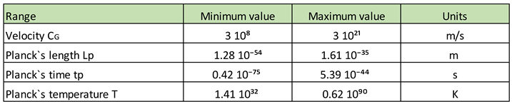
Electromagnetic Planck´s constants:
Cɛ = 3 x 10⁸ m/s
Lpɛ = 1.61 10⁻³⁵ m
tpɛ = 5.39 10⁻⁴⁴ s
Tpɛ = 1.41 10³² K
Gravitational Planck´s constants:
Cɢ = 3 x 10⁸ m/s to 3 x 10²¹ m/s
Lpɢ = 1.61 10⁻³⁵ m to 1.28 10⁻⁵⁴ m
tpɢ = 5.39 10⁻⁴⁴ s to 0.426 10⁻⁷⁵ s
Tpɢ = 1.41 10³² K to 0.62 10⁹⁰ K
Analysing Table 2, it is important to highlight the following: at time T0⁺, at the moment the black hole disintegrates, the Planck´s length corresponds to Lpɢ = 1.28 10⁻⁵⁴ m. At time t → infinity, the Planck´s length takes the value of Lpɛ = 1.61 10⁻³⁵.
Example:
Let us refer again to equations (8), (9) and (10).
We have no problem interpreting equation (8) and (9).
Equation (9) is given by the following condition:
R > Rs, v < c; ds < 0, time type trajectory
It tells us that any particle outside a black hole is going to move at a speed less than the speed of light c, (c – v > 0; v < c).
Equation (8) given by:
R = Rs, v = 0; ds² = 0; Rs is the Schwarzschild´s radius
It tells us that any particle that reaches the event horizon of a black hole will move at the speed of light c, that is, its net speed (c - v = 0; c = v).
Condition (10) given by:
R < Rs, v > c; ds > 0, space type trajectory
Any particle inside a black hole, R < Rs; moves at a speed greater than c, that is, (v - c > 0; v > c).
To interpret this, we will use the Lorentz equations for length and time.
Length and Time, for v < c:
L = L0 √ [1 – (v/c) ²], T = T0 / √ [1 – (v/c) ²]; for time type trajectory
L0 represents the length of a particle at rest, as the particle increases its speed, its length L decreases, a contraction occurs.
For v > c
L = i L0 √ [(v/c) ² -1], T = - i T0 / (√ [(v/c) ² -1); for space type trajectory.
Let's interpret the meaning when we say that L goes from a time-type trajectory to a space-type trajectory:
This means that L takes the form of the equation of T, as follows:
L = - i L0 / [√ [(v/c) ² -1]
True equation of (L) inside a black hole
Where i represents the imaginary number.
This makes perfect sense, as v > c; L (Lpɢ) takes values smaller than the Planck´s length (Lpɛ), we are considering L0 = Lpɛ = Planck´s length. If we had not made the change in the equation, as v > c, L would have started to grow again and this contradicts our assumption that as a black hole grows, the Planck´s length inside it decreases.
Let's go back to the black hole analogy, consider a particle falling into a black hole moving towards the center of mass, once it crosses the event horizon, v > c, therefore the length equation takes the following value: L = i L0 / √ [(v/c) ² -1]. Looking at the equation, we can conclude the following:
First, as v grows with respect to c, L decreases below the value of L0 (it takes values smaller than the Planck´s length).
Second, when the particle passes the event horizon and enters the interior of the black hole, we see that the imaginary number i appears in the equation, this can be interpreted as the particle stops heading towards the interior of the black hole and begins to move in circles around the center of the black hole as a particle does in the Kerr black hole. The imaginary number i tells us that the direction of the particle is 90 degrees with respect to the previous direction, towards the center of mass of the black hole.
Finally, we will interpret what has been stated, using the following graph:
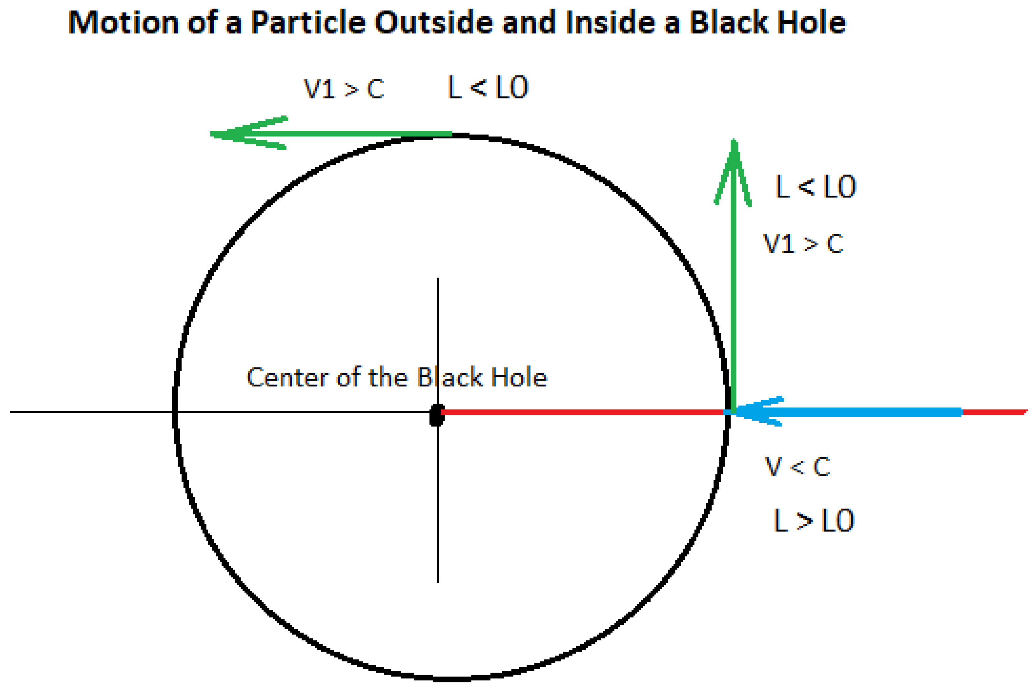
Figure 6.
The red line, indicated by the blue arrow, can be interpreted as the motion of a particle falling into a black hole. As it passes the event horizon, we see that the particle acquires a rotational motion, orthogonal to the direction toward the interior of the black hole; indicated by the green arrow.
2.5. Modelling the Planck´s Length Expansion as a Function of Redshift (z).
In order to determine our model that describes how the Planck length varies as a function of redshift, it is necessary to analyse the wave equation of the universe.
Here, we are going to present a mathematical development that I carried out in another paper, but it is necessary to be able to understand the model that we are going to propose: Planck´s length variation as a function of the redshift (z).
E (t) = 1.08 10⁷³ {e ⁻ (1.81 10⁻¹¹ t)} – 1.08 10⁷³ {e ⁻ (2.19 10¹¹ t)} + E0
Where E0 corresponds to the temperature of 2.7 K
This equation represents: the gravitational wave equation of the universe.
λ = 1.000.000 Light years = 10⁶ x 9.46 10¹⁵ m
Where, λ is the fundamental wavelength
λ is a data provided by the IFT UAM.
λ = 9.46 10²¹ m
c = λ x f, f = c/λ, f = 3 10²¹ / 9.46 10²¹ = 0.317 Hz
f = 0.317 Hz
Where, f is the fundamental frequency
ω = 2.ᴨ.f = 2 x 3.14 x 0.317 = 2
ω = 2.00 rad/s
Where, ω is the fundamental angular frequency
We will calculate: ω0, B, ω1 and ω2 for our RLC circuit.
R = 3.60 10⁵¹ Ohms
L = 1.98 10⁶² Hy
C = 1.26 10⁻⁶³ F
ω0 = 1 / √ LC rad/s
ω0 = 1 / √ LC = 1 / √ (1.98 10⁶² Hy x 1.26 10⁻⁶³ F) = 1 / √2.49 x 10⁻¹
ω0 = 2.00 rad/s
Where ω0, is the resonance frequency or fundamental angular frequency.
We will calculate the high cut-off frequency:
ω2 = + 1 / 2RC + √ (1 / 2RC) ² - (1 / LC)
S2 = - α - √ (α) ² - (ω0) ²
ω2 = 11.00 10¹⁰ + √ (121.00 10²⁰ - 4)
ω2 = 2.19 10¹¹ rad/s
ω2 is the high cut-off frequency
ω2 = 2.19 10¹¹ rad/s
f2 = ω2 / 2π = 2.19 10¹¹ / 2 x 3.14 = 0.348 10¹¹
f2 = 0.348 10¹¹ Hz
λ2 = C / f2 = 3 10²¹ / 0.348 10¹¹ = 8.60 10¹⁰
λ2 = 8.60 10¹⁰ m
We will calculate the low cut-off frequency:
ω1 = -1 / 2RC + √ (1 / 2RC) ² + (1 / LC)
S1 = - α + √ ((α)² - (ω0) ²)
ω1 = -11.00 10¹⁰ + √ (121.00 10²⁰ - 4)
ω1 = 1.81 10⁻¹¹ rad/s
where, ω1 is the low cut-off frequency
ω1 = 1.81 10⁻¹¹ rad/s
f1 = ω1 / 2π = 1,81 10⁻¹¹ rad/s / 2 x 3.14 = 2.88 10⁻¹²
f1 = 2.88 10⁻¹² Hz
λ1 = C / f1 = 3 10²¹ / 2.88 10⁻¹² = 1.08 10³³
λ1 = 1.08 10³³ m
We will calculate the bandwidth:
B = ω2 - ω1
B = 2.2 10¹¹ rad/s
B is the bandwidth
It is always good to remember that the energy stabilizes when the space reaches 2.7 K, which corresponds to 3.72 10⁻²³ J.
3.72 10⁻²³ = 1.08 10⁷³ e⁻ (1.81 10⁻¹¹ t)
e⁻ (1.81 10⁻¹¹ t) = 0.290 10⁹⁶
1.81 10⁻¹¹ t = ln (0.290 10⁹⁶)
t = ln (0.290 10⁹⁶) / 1.81 10⁻¹¹ = 219.84 / 1.81 10⁻¹¹ = 121.46 10¹¹
t = 1.22 10¹³ s
Where, t is the time in which the equation E(t) reaches 2.7 K
At t = 1.22 10¹³ s, space-time has expanded by a factor of:
e = v x t
e = 1.22 10¹³ s x 3 10²¹ m/s = 3.66 10³⁴ m.
e = 3.66 10³⁴ m
We will calculate the number of seconds in 380,000 years:
t = 11.81 10¹² s
We will analyse Figure 7:
- low cut-off frequency: ω1 = 1.81 10⁻¹¹ rad/s
- High cut-off frequency: ω2 = 2.19 10¹¹ rad/s
- Fundamental or resonant frequency: ω0 = 2.00 rad/s
- Bandwidth: B =2.2 10¹¹ rad/s
- Space travelled that corresponds to the total bandwidth: e = 3.66 10³⁴ m
- Minimum time: approximately t = 10ˉ¹³ s
- Maximum time: t = 1.22 10¹³ s
Now we are going to analyse something very important; will help us understand the origin of dark energy.
We said, to form a black hole, the Boltzmann´s constant changes from Kʙ = 1.38 10ˉ²³ J/K (flat space-time) to Kʙ = 1.78 10ˉ⁴³ J/K (curved space-time). once the black hole forms the Boltzmann´s constant remains constant at Kʙ = 1.78 10ˉ⁴³ J/K. As the black hole grows, the Planck´s length varies from Lpɢ = 1.61 10⁻³⁵ m to 1.28 10⁻⁵⁴ m. When it reaches the Planck´s length Lpɢ = 1.28 10⁻⁵⁴ m, the speed of massless particles inside a black hole is c = 10²¹ m/s.
How can we relate the statement to the Big Bang? Let's try to interpret this as follows:
If we imagine the Planck length behaving like a spring, as a black hole grows, the Planck length decreases, meaning the spring decreases in size, increasing its gravitational potential energy.
When the black hole disintegrates and the Big Bang occurs, the Planck´s length that was at the value of Lpɢ = 1.28 10⁻⁵⁴ m tends to reach its normal or stable value of Lpɛ = 1.61 10⁻³⁵ m, expanding at a speed of c = 10²¹ m/s, generating cosmic inflation.
In the first instance, each generated frequency, shown in the bandpass circuit in Figure 7, must travel a distance e = 3.66 10³⁴ m, which brings the total time to 10²⁶ s. Example, the fundamental frequency that originates in 1 s, goes up to 1.22 10¹³ s; the last frequency that originates in 1.22 10¹³ s, goes up to 10²⁶ s; where each of the frequencies of the spectrum travels a distance e = 3.66 10³⁴ m.
This is the first event that contributes to the origin of dark energy; each generated gravitational wave travels at a speed c = 10²¹ m/s and travels a space of e = 3.66 10³⁴ m.
We will analyze the second event that will help us understand dark energy even more.
The second event is related to the Boltzmann´s constant, in this process the Boltzmann´s constant Kʙɢ = 1.78 10ˉ⁴³ J/K (curved space-time) must reach the value of Kʙɛ = 1.38 10ˉ²³ J/K (flat space-time), In this process each gravitational wave travels at the speed of light c = 3 10⁸ m/s
In the second event, we will propose that the shape of the CMB power spectrum will determine the shape of the energy contribution of gravitational waves produced in the early Universe, which will determine how the Universe will expand.
Both events are important and give rise to dark energy.
Finally, considering the statement above, in the following graph we will try to represent the energy (E(t) vs t(s)) and (H(t) vs t(s)).
In Figure 8 and Figure 9, the X axis is represented to scale, the y axis is not represented to scale.
In Figure 8, I try to represent the contribution of the energy of gravitational waves up to a time t = 10²⁶ s.
In Figure 9, I try to represent the variation of the Hubble´s constant up to a time t = 10²⁶ s, considering the energy contribution of gravitational waves.
Observing Figure 9, we see that from t = 10¹² s, there is an inflection point in which the Hubble´s constant goes from negative to positive slope, this is due to the gravitational wave front, which has the shape of the frequency spectrum distributed in time, figure 8, which adds energy, causing the universe to go from decelerated expansion to accelerated expansion. This is manifested by a variable Hubble´s constant as shown in Figure 9.
We also observe for t = 10²⁶ s, Figure 9, another inflection point occurs due to the absence of gravitational waves, as shown in Figure 8, in which the slope is zero (horizontal).
It is very important to make clear that the accelerated expansion of the universe has a limit and it is given for t = 10²⁶ s, after that time, space-time stabilizes.
If we measure the Hubble´s constant using the 1A supernova method, it gives us: H = 74 km/s/Mpc.
If we measure the Hubble´s constant, using the CMB microwave radiation background, it gives us: H = 67 km/s/Mpc.
If we measure the Hubble´s constant using merged neutron stars, using the electromagnetic spectrum and gravitational waves, it gives us: H = 66.2 km/s/Mpc.
If we measure the Hubble´s constant using an 1A supernova and gravitational lensing, it gives us: H = 64 km/s/Mpc.
Which of these measurements is correct? Or are all measurements correct?
Possibly the measurements of the Hubble´s constants determined by the four different methods are correct and the difference between the calculated measurements for the Hubble´s constants is due to the fact that the expansion of space-time is different in each place where the measurements are carried out, because the measurements were made in different time periods of the expansion of the space-time of the universe, as shown in Figure 9, which represents the variation of the Hubble´s constant H vs t.
Example 1:
According to Figure 9, if we divide by power of 10, logarithmic scale, we have approximately 26 steps, neglecting negative exponent stages.
Let's calculate the time t, today.
t = 4.35 10¹⁷ s, correspond to 17.5 steps.
(17.5 / 26) x 100 = 67.3%
This is similar to the dark energy content of the universe that scientists have calculated.
100% - 67.3 = 32.7 %
This is similar to the dark matter content of the universe that scientists have calculated.
We will calculate the number of seconds in 380,000 years:
t = 11.81 10¹² s
We will calculate the number of seconds it will take for the universe to stabilize and reach a temperature of 2.7 K.
t = 1.22 10¹³ s
If we perform the following quotient, we obtain:
(11.81 10¹² s / 1.22 10¹³ s) x 100 = 96.72 %
100% - 96,72% = 3.28%
Baryonic matter content in the universe.
The true interpretation of this result is the following: the fundamental wavelength that corresponds to λ = 1,000,000 light years, represents the highest amplitude peak of the CMB power spectrum, has convolved 96% with the space-time of the universe and still needs to be convolved 4%.
The following values:
Dark energy = 67.3%
Dark matter = 29.42 %
Baryonic matter = 3.28 %
Represent the proportions of dark energy, dark matter and baryonic matter of the fundamental frequency referenced to the moment of time t that corresponds to the CMB.
If we consider the contribution of the frequencies that make up the power spectrum, the percentage values of dark energy, dark matter, and baryonic matter should change.
After this excellent introduction, we are now able to model the expansion of the Planck´s length as a function of redshift z.
For T0⁺ → Lpɢ = 1.28 10⁻⁵⁴ m
For T → infinito, Lpɢ = Lpɛ = 1.61 10⁻³⁵ m
Here, we are going to analyze something very important.
If we look at Figure 8, today corresponds to a time of 5 10¹⁷ s.
If we look at Figure 8, the moment at which the perturbations of the gravitational waves stabilize corresponds to 10²⁶ s.
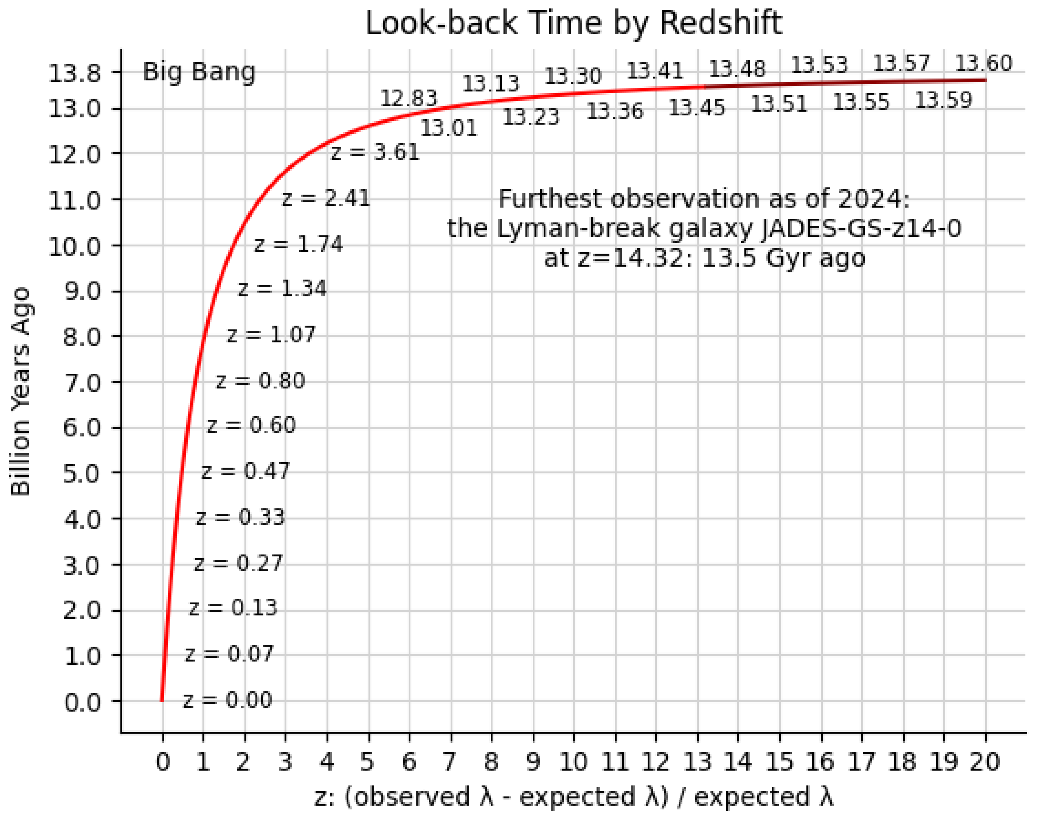
If we look at Figure 2, the y-axis is represented by the time in billions of years; the x-axis is represented by the redshift z. It should be noted that the time corresponding to 13.8 (5 10¹⁷ s) billion years represents a fraction of the total time corresponding to 10²⁶ s.
If we consider the power of 10, we can represent 10²⁶ s as 26 steps. Today's time, which corresponds to 5 10¹⁷ s, corresponds to 17.5 steps.
We carry out the following quotient:
(17.5 / 26) % = 67.30 %
Now let's consider the Planck´s length:
For T0⁺ → Lpɢ = 1.28 10⁻⁵⁴ m
For T → infinite, Lpɢ = Lpɛ = 1.61 10⁻³⁵ m
If we consider 10⁻⁵⁴ m to 10⁻³⁵ m, there are 19 steps in power of 10.
We make the following calculation:
(19 x 67.30) / 100 = 12.8
This tells us that as of today, the Planck´s length has increased from 10⁻⁵⁴ m to 10⁻⁴² m. In the time between 5 10¹⁷ s and 10²⁶ s, the Planck´s length will increase from 10⁻⁴¹ m to 1.61 10⁻³⁵ m.
After this explanation, we have found the way to model the Planck´s length as a function of the redshift z.
We are going to propose the following model.
For the model represented by the blue line (Figure 10), equation (1) can be represented as follows:
We observe that in the model represented by the blue line (Figure 10), the constant Tau, τ = RC = 2.
For the model represented by the green line (Figure 10), equation (1) can be represented as follows:
We observe that in the model represented by the green line (Figure 10), the constant Tau, τ = RC = 3.
We observe that redshift with the blue line model is more similar to the redshift model with the red line.
Let's perform the following calculations to determine how the Planck´s length calculation works and how it relates to redshift.
We use equation 17:
τ = z = 2
If we go to Figure 7, for the model represented by the blue line, Q (2) = 8.4
8.4 corresponds to an equivalent Planck´s length of 10⁻⁴⁹ m
For T0⁺, z →infinite, Lpɢ → 1.28 10⁻⁵⁴ m
For t → 0, z →0, Lpɢ → 10⁻⁴² m
We use equation 18:
τ = z = 3
If we go to Figure 7, for the model represented by the green line, Q (3) = 9.0
(9.0) corresponds to an equivalent Planck´s length of 10⁻⁵⁰ m
For T0⁺, z →infinite, Lpɢ → 1.28 10⁻⁵⁴ m
For t → 0, z →0, Lpɢ → 10⁻⁴² m
Now we are going to make a new model: comoving distance vs redshift
For this we will use the following graph:
We are going to model the comoving distance vs. redshift, using the capacitor charge model, which follows the Tau curve.
It is observed that the orange dotted line corresponds to the model we proposed in Figure 10, which corresponds to look-back time vs. redshift (z).
In this stage, we will model comoving distance vs redshift (z), following the charge curve of a capacitor, which follows the law of the Tau constant.
In the following graph we will interpret and execute our modelling in the following way:
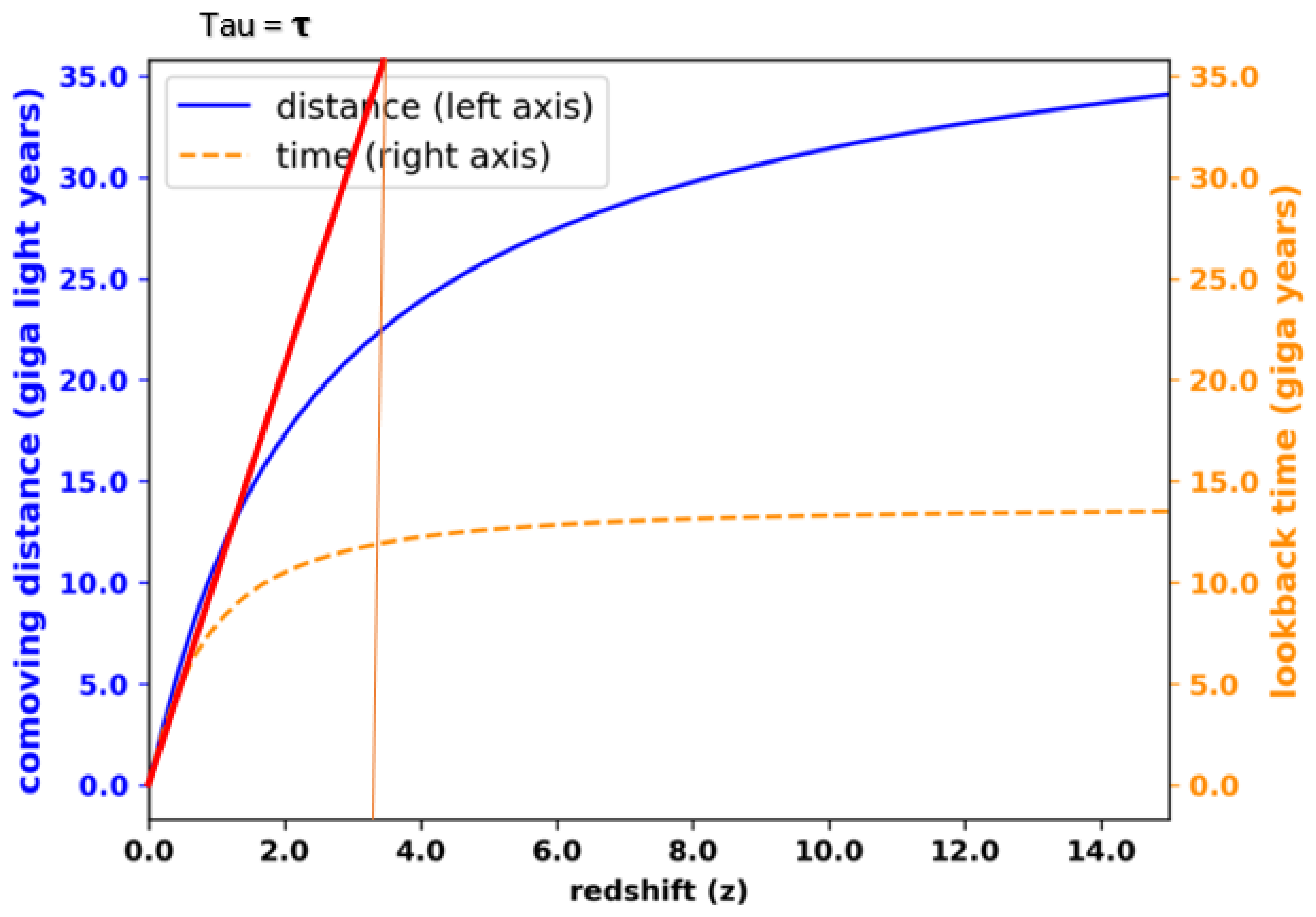
Figure 12.
comoving distance vs redshift z modelling.
For the model represented by blue line, equation (1) can be represented as follows:
In our model Tau corresponds to approximately (z = 3.5).
Remember that 35 corresponds to 35 giga light years (a measure of distance).
Now we are going to perform the following modelling: variation of the Planck´s length versus redshift (z).
For this we will use the following graph:
For the model in blue, equation (1) can be represented as follows:
True equation which represents the Planck´s length variation using comoving distance versus red shift z.
If we compare equation (17) and (18) represented by Figure 10 with equation (20) represented by Figure 13; in my personal opinion, I think that the model: variation of the Planck length versus redshift (z) given by equation (20) is the correct model and represents more accurately the variation of the Planck´s length versus redshift (z).
If we compare the blue line versus the orange dotted line in Figure 13, we see that the blue line more closely resembles the charge of a capacitor. In Figure 10, for the defined constants Tau; 5Tau does not represent the full charge value as required in the theory of a capacitor charging circuit, however, the constant Tau defined in equation (20) given in Figure 10; more closely resembles a capacitor charging circuit.
3. Conclusions
In a first instance, we have shown that we can model the time evolution in millions of light-years as a function of redshift z. To do this, we used the charge model of an RC capacitor, which charges according to a constant Tau.
In equation 2, the constant Tau = 2; in equation 3, the constant tau = 3.
This is an approximate model; it is not exact, but it gives us a good idea of the time evolution of the universe as a function of redshift z.
We subsequently developed the mathematical evolution of the Planck´s length inside a black hole from another paper, and demonstrated that as a black hole grows, the Planck´s length decreases; this occurs until the black hole reaches its critical mass and, at time T0⁺, disintegrates, generating the Big Bang.
As stated, at time T0⁺, the Planck´s length is equal to Lpɢ = 1.28 10⁻⁵⁴ m. We said that the Planck´s length is equal to a spring, therefore, after the decay of a black hole, the Planck length, which was initially Lpɢ = 1.28 10⁻⁵⁴ m, will try to reach the value of Lpɛ = 1.61 10⁻³⁵ m.
Here comes our second proposed model, which consists in modelling the expansion of the Planck´s length from Lpɢ = 1.28 10⁻⁵⁴ m to Lpɛ = 1.61 10⁻³⁵ m (Look Back Time versus redshift z) similar to the charge of an RC circuit. See Figure 10.
Finally, we will present our third proposed model, our goal: variation of the Planck´s length using the comoving distance versus redshift (z), see Figure 13, represented by equation 20.
We present three proposed models: equation 17 with the constant (Tau = 2), equation 18 with the constant (Tau = 3) and equation 20 with the constant (Tau = 3.5). The models are not exact, but they give a good approximation of the evolution of the Planck´s length as a function of redshift z.
It is important to clarify that the first two models represent: variation of the Planck´s length (Lookback time) vs. Redshift (z); the third model represents: variation of the Planck´s length (Comoving Distance) vs. Redshift (z).
The third model: variation in the Planck´s length using the comoving distance vs. redshift (z), given by equation 20; is the most accurate model and most faithfully represents the charge curve of a capacitor.
I think we can now better understand the true meaning of vacuum energy, dark energy, and understand exactly how the Planck´s length plays a role in this process. This also explains the discrepancy with the Hubble constant.
About the Authors
HECTOR GERARDO FLORES (ARGENTINA, 1971). I studied Electrical Engineering with an electronic orientation at UNT (Argentina); I worked and continue to work in oil companies looking for gas and oil for more than 25 years, as a maintenance engineer for seismic equipment in companies such as Western Atlas, Baker Hughes, Schlumberger, Geokinetics, etc.
Since 2010, I study theoretical physics in a self-taught way.
In the years 2020 and 2021, during the pandemic, I participated in the course and watched all the online videos of Cosmology I and Cosmology II taught by the Federal University of Santa Catarina UFSC (graduate level).
MARIA ISABEL GONÇALVEZ DE SOUZA (BRAZIL, 1983). I studied professor of Portuguese language at the Federal University of Campina Grande and professor of pedagogy at UNOPAR University, later I did postgraduate, specialization. I am currently a qualified teacher and I work for the São Joao do Rio do Peixe Prefecture, Paraiba. I am Hector's wife and my studies served to collaborate in the formatting of his articles, corrections, etc; basically, help in the administrative part with a small emphasis in the technical part analysing and sharing ideas.
Conflicts of Interest
The author declares that there are no conflicts of interest.
References
- Flores, H. G. (2023). RLC electrical modelling of black hole and early universe. Generalization of Boltzmann's constant in curved spacetime. J Mod Appl Phys. 2023; 6(4):1-6. https://www.preprints.org/manuscript/202305.2246/v3.
- Flores, H. G.; Gonçalvez de Souza, M. I. Theory of the Generalization of the Boltzmann’s Constant in Curved Space-Time. Shannon-Boltzmann Gibbs Entropy Relation and the Effective Boltzmann’s Constant. Preprints 2023, 2023090301. [CrossRef]
- Flores, H. G.; Gonçalves de Souza, M. I. RC Electrical Modelling of Black Hole. New Method to Calculate the Amount of Dark Matter and the Rotation Speed Curves in Galaxies. Preprints 2023, 2023092017. [CrossRef]
- Flores, H. G.; Jain, H.; Gonçalves de Souza, M. I. Origin of the Dark Energy. Preprints 2024, 2024051639. [Google Scholar] [CrossRef]
- Flores, H. G.; Jain, H.; Mahapatra, P.; Gonçalves de Souza, M. I. Analysis of the Kerr-Newman Diagram. Unravelling the Interior of a Black Hole. Preprints 2024, 2024080101. [Google Scholar] [CrossRef]
- Circuito RC: Processo de Carga e Descarga de Capacitores Departamento de Física - ICE – UFJF https://www2.ufjf.br/fisica/wp-content/uploads/sites/427/2010/03/A06-Circuito-RC-2015-10-21.pdf.
- Redshift From Wikipedia https://en.wikipedia.org/wiki/Redshift.
- Planck Length and Cosmology Xavier Calmet, Modern Physics Letters A.https://arxiv.org/pdf/0704.1360.
- Dynamically Induced Planck Scale and Inflation Kristjan Kannike, Gert Hutsi, Liberato Pizza, Antonio Racioppi, Martti Raidal, Alberto Salvio, and Alessandro Strumia. IFT-UAM/CSIC-15-015 https://arxiv.org/pdf/1502.01334.
- Micro Black Hole Candidates and the Planck Scale Espen Gaarder Haug and Gianfranco Spavieri https://papers.ssrn.com/sol3/papers.cfm?abstract_id=4856325 file:///C:/Users/55839/Downloads/ssrn-4856325%20(1).pdf.
- Effective Planck mass and the scale of inflation Journal of Cosmology and Astro-particle Physics, IOP. https://iopscience.iop.org/article/10.1088/1475-7516/2016/01/017/pdf.
- Planck stars, White Holes, Remnants and Planck-mass quasi-particles. The quantum gravity phase in black holes’ evolution and its manifestations Carlo Rovelli and Francesca Vidotto https://arxiv.org/html/2407.09584v2.
- Too Hot to Handle: Searching for Inflationary Particle Production in Planck Data Oliver H. E. Philcox, Soubhik Kumar and J. Colin Hill https://arxiv.org/html/2405.03738v2.
- The Planck length as a duality of the Cosmological Constant: S-dS and S-AdS thermodynamics from a single expression Ivan Arraut https://arxiv.org/abs/1205.6905.
- Warm-tachyon Gauss-Bonnet inflation in the light of Planck 2015 data Maysam Motaharfar, Hamid Reza Sepangi https://arxiv.org/abs/1604.00453.
- Tachyon-Warm Intermediate and Logamediate Inflation in the Brane-World Model in the Light of Planck Data Vahid Kamali, Mohammad Reza Setare https://arxiv.org/abs/1508.05479.
- High Energy Physics – Theory https://arxiv.org/list/hep-th/new.
- Cosmology at high redshift -- a probe of fundamental physics Noah Sailer, Emanuele Castorina, Simone Ferraro, Martin White https://arxiv.org/abs/2106.09713.
- High-Redshift Cosmography Vincenzo Vitagliano (SISSA and INFN, Trieste), Jun-Qing Xia (SISSA, Trieste), Stefano Liberati (SISSA and INFN, Trieste), Matteo Viel (INFN and INAF-Osservatorio Astronomico di Trieste) https://arxiv.org/abs/0911.1249.
- Cosmology with large redshift surveys Laerte Sodre Jr https://arxiv.org/abs/1212.1576.
- Cosmographic analysis of redshift drift Francisco S. N. Lobo, Jos´e Pedro Mimoso and Matt Visser https://arxiv.org/pdf/2001.11964.
- High-redshift cosmography with a possible cosmic distance duality relation violation José F. Jesus, Mikael J. S. Gomes, Rodrigo F. L. Holanda, Rafael C. Nunes. https://arxiv.org/html/2408.13390v3.
- Dark Energy with Phantom Crossing and the H0 tension Eleonora Di Valentino, Ankan Mukherjee, Anjan A. Sen https://cosmocoffee.info/viewtopic.php?t=3355&sid=ae714d9643fd6ee13c29d2c85da9d1af.
Figure 3.
charging process of a capacitor.
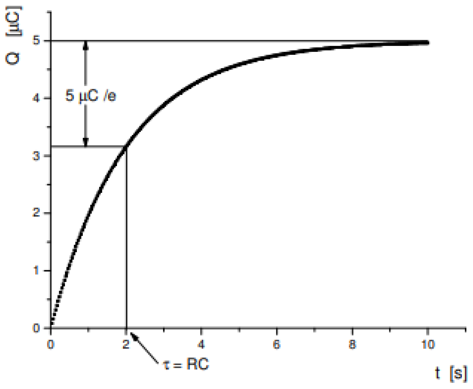
Figure 4.
In blue and green are represented two models proposed to model the redshift (z) in red.
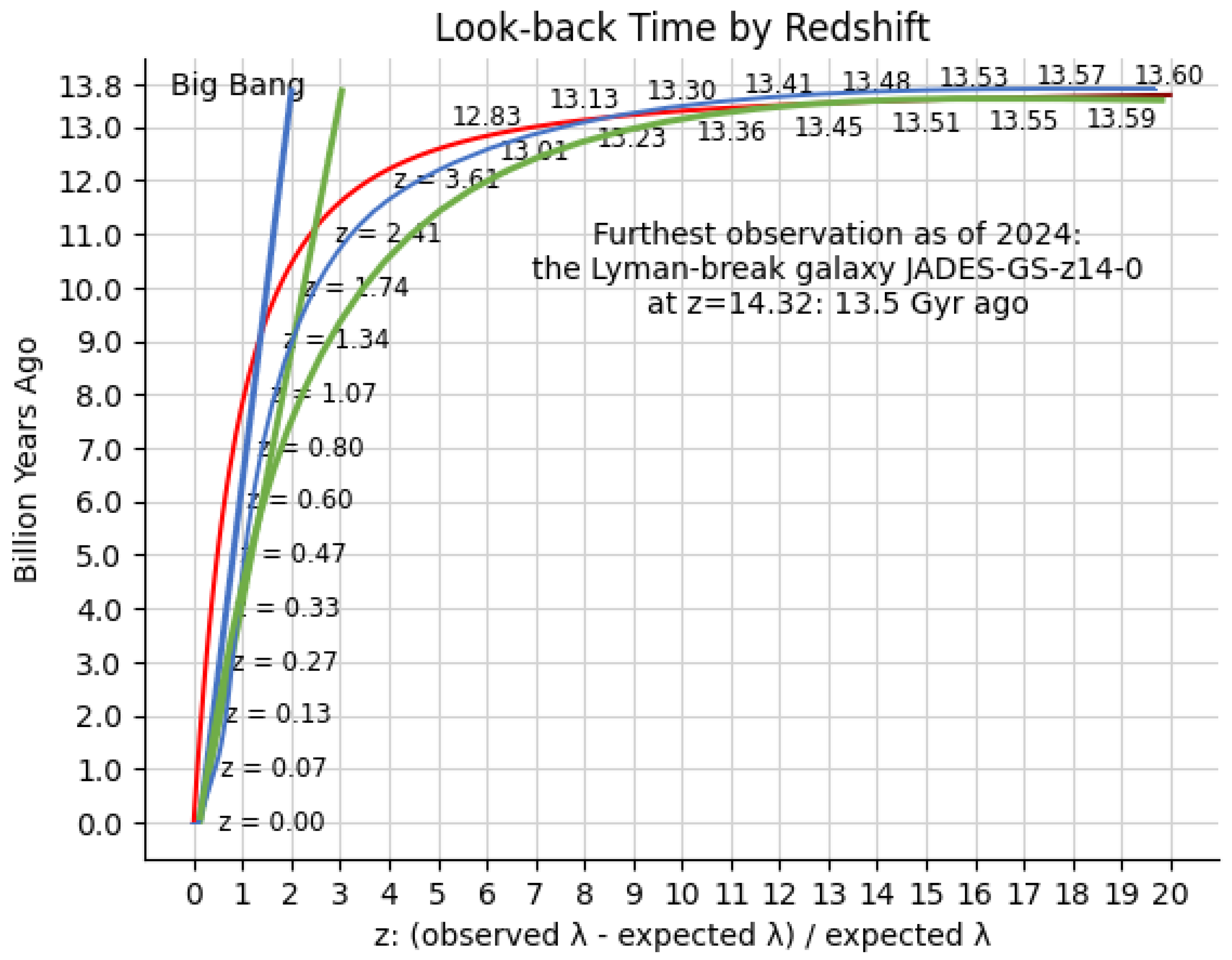
Figure 5.
Represents the variation of speed Cɢ, as a function of temperature T, inside a black hole.
Figure 5.
Represents the variation of speed Cɢ, as a function of temperature T, inside a black hole.
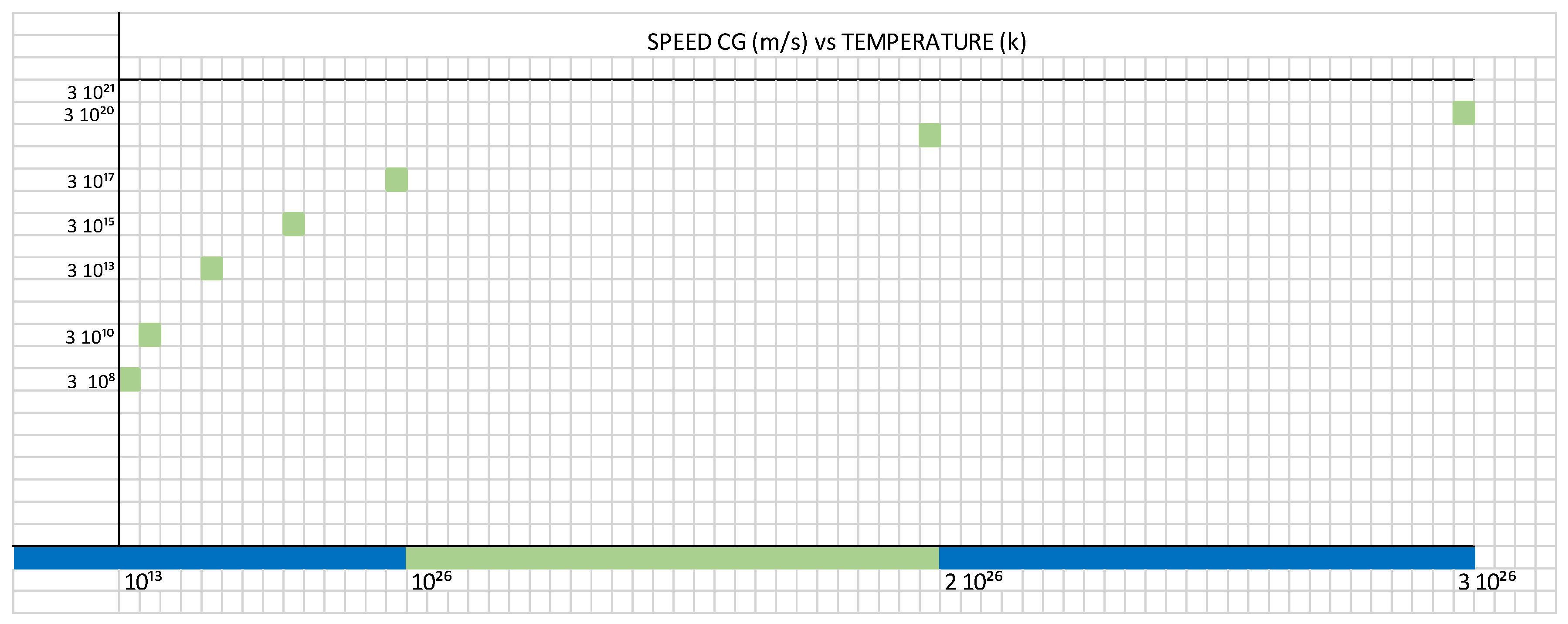
Figure 7.
Spectrum of gravitational waves produced in the cosmic inflation.
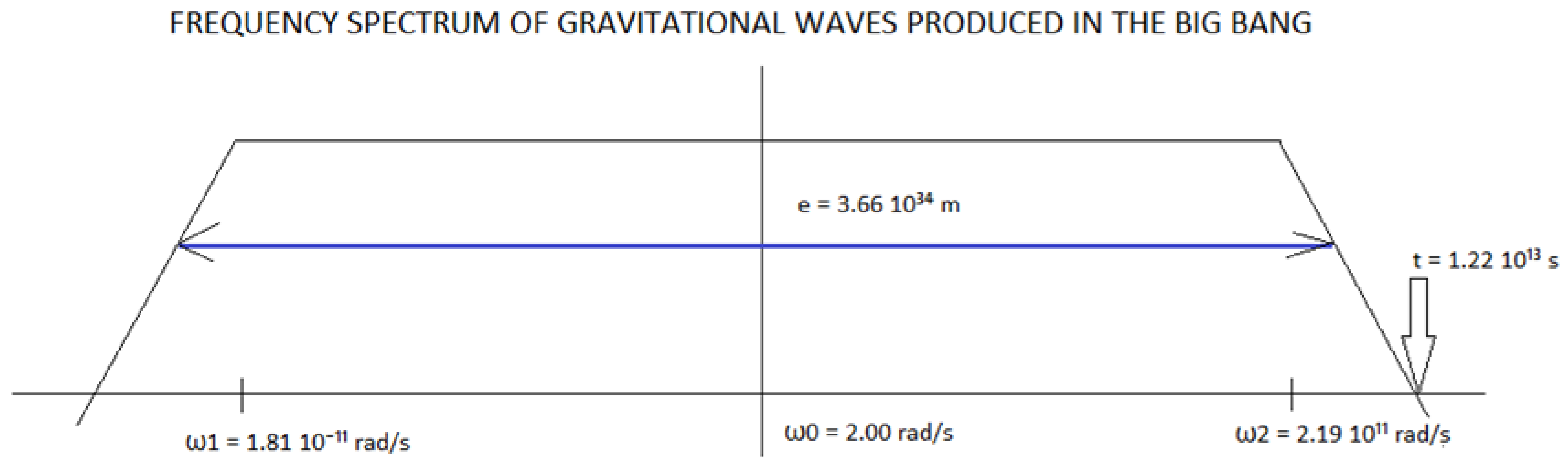
Figure 8.
In blue, it represents the energy contribution of gravitational waves versus time, it is observed for t = 10²⁶ s, the energy contribution of gravitational waves becomes zero (0).
Figure 8.
In blue, it represents the energy contribution of gravitational waves versus time, it is observed for t = 10²⁶ s, the energy contribution of gravitational waves becomes zero (0).
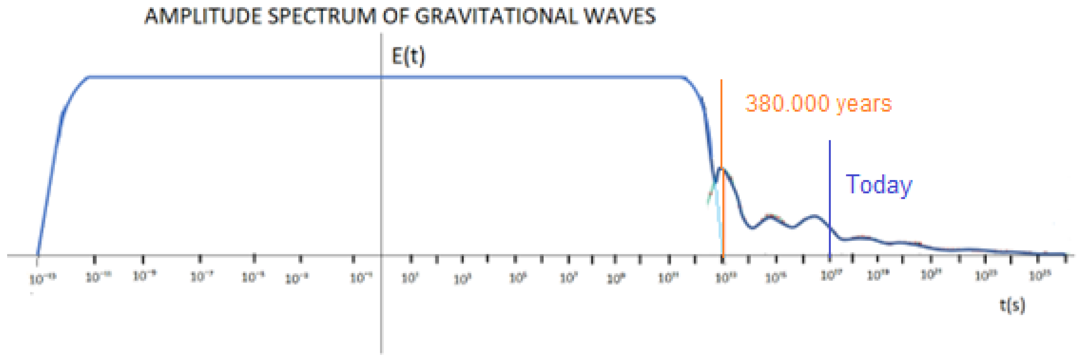
Figure 9.
In orange, it represents the variation of the Hubble´s constant versus time, for t = 10²⁶ s, the Hubble´s constant becomes zero (0).
Figure 9.
In orange, it represents the variation of the Hubble´s constant versus time, for t = 10²⁶ s, the Hubble´s constant becomes zero (0).
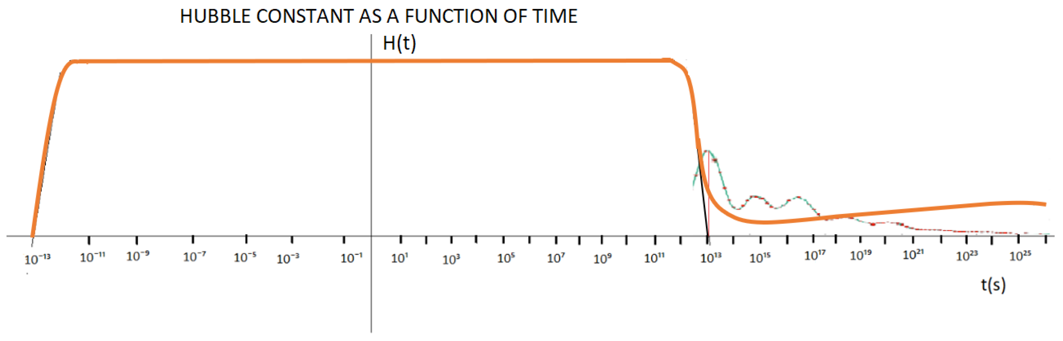
Figure 10.
On the y-axis, we have the representation of time in billions of years, which is equivalent to the Planck´s length variation. On the x-axis, it is represented by the redshift (z).
Figure 10.
On the y-axis, we have the representation of time in billions of years, which is equivalent to the Planck´s length variation. On the x-axis, it is represented by the redshift (z).
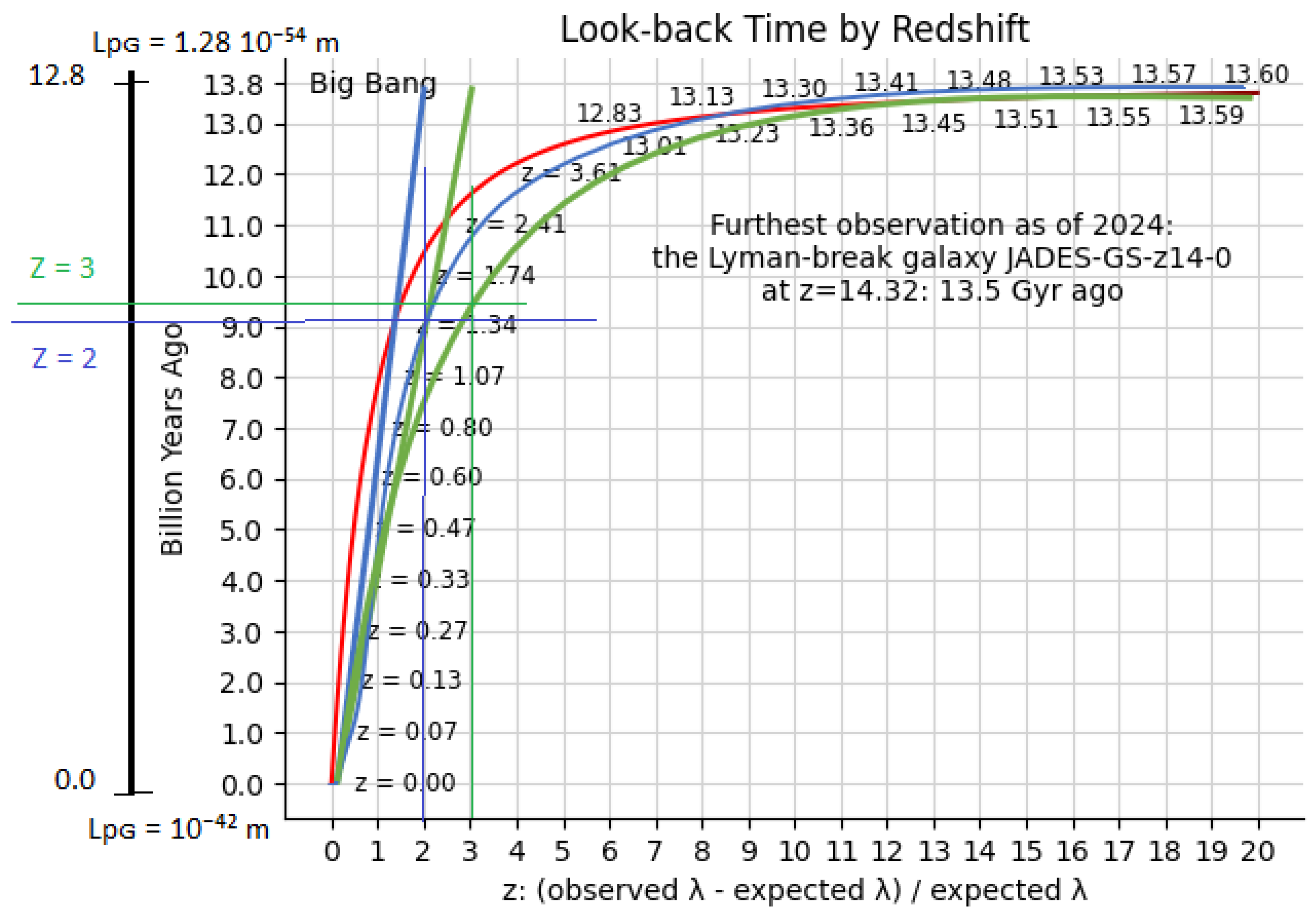
Figure 11.
comoving distance vs redshift z.
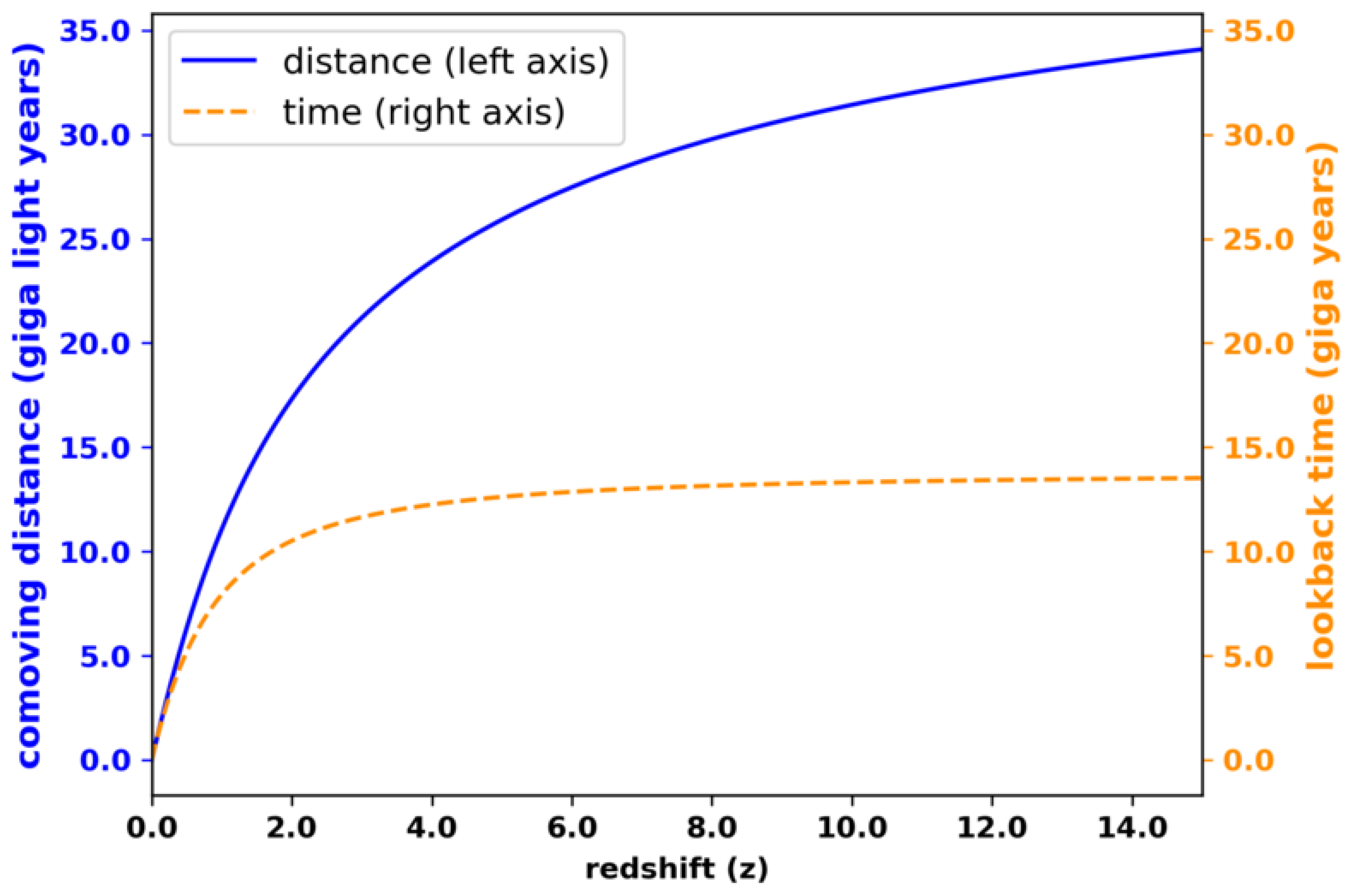
Figure 13.
Planck´s length variation versus redshift (z).
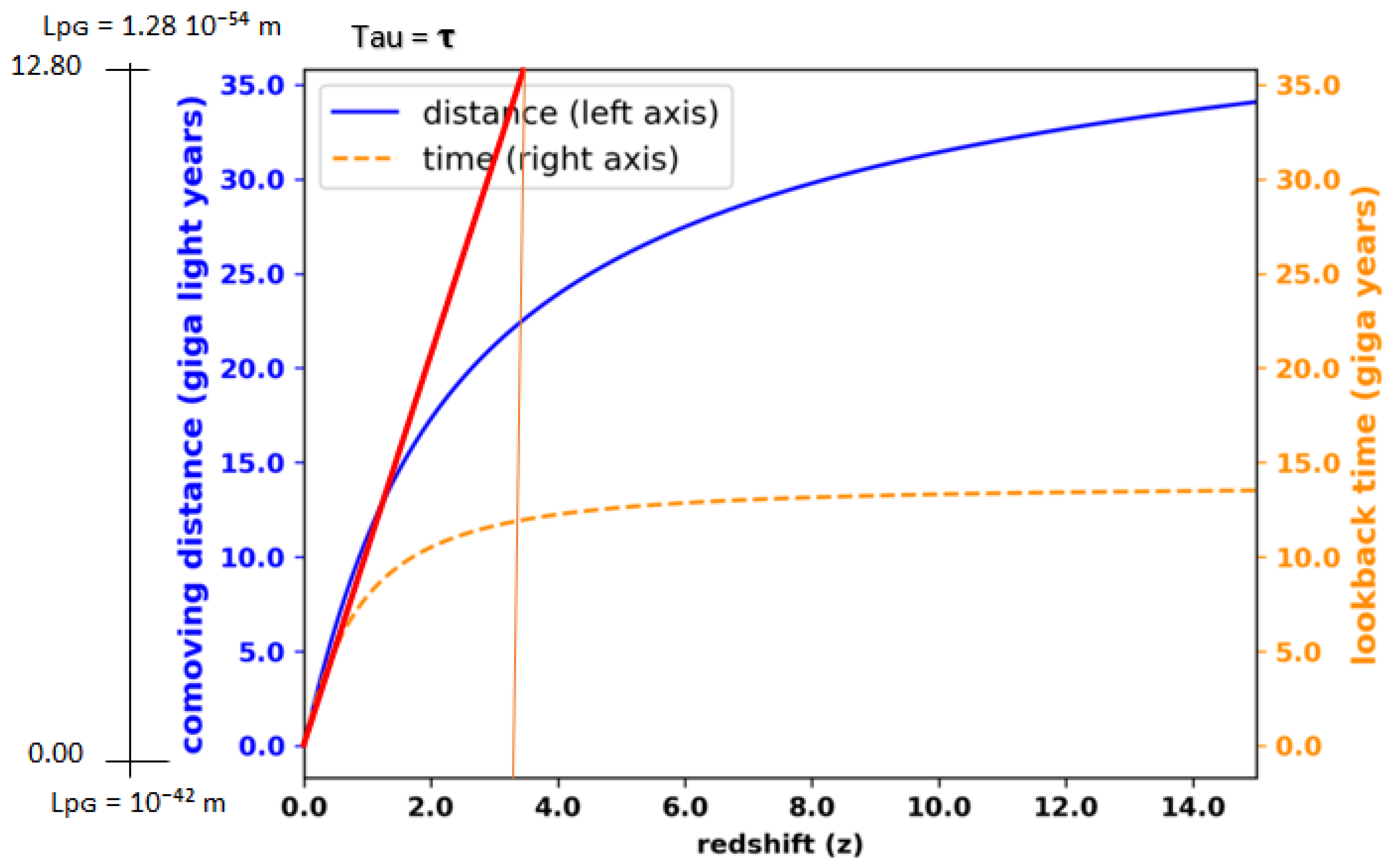

Table 1.
Represents values of ImI, baryonic mass; IδI, dark matter mass; IMI, mass of baryonic matter plus the mass of dark matter; IEmI, energy of baryonic matter; IEδI, dark matter energy; IEI, Sum of the energy of baryonic matter plus the energy of dark matter and Rs, Schwarzschild´s radius, as a function of, c, speed of light; Cɢ, speed greater than the speed of light; T, temperature in Kelvin; using the parametric equations.
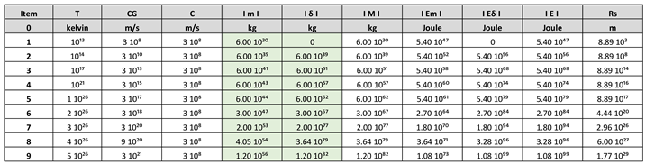 |
Table 2.
We represent the range of variation of the velocity C, the Planck´s length, the Planck´s time and the Planck´s temperature.
Table 2.
We represent the range of variation of the velocity C, the Planck´s length, the Planck´s time and the Planck´s temperature.
 |
Disclaimer/Publisher’s Note: The statements, opinions and data contained in all publications are solely those of the individual author(s) and contributor(s) and not of MDPI and/or the editor(s). MDPI and/or the editor(s) disclaim responsibility for any injury to people or property resulting from any ideas, methods, instructions or products referred to in the content. |
© 2025 by the authors. Licensee MDPI, Basel, Switzerland. This article is an open access article distributed under the terms and conditions of the Creative Commons Attribution (CC BY) license (http://creativecommons.org/licenses/by/4.0/).
Copyright: This open access article is published under a Creative Commons CC BY 4.0 license, which permit the free download, distribution, and reuse, provided that the author and preprint are cited in any reuse.


