
Submitted:
30 May 2025
Posted:
04 June 2025
You are already at the latest version
Abstract
The instabilities in time and frequency transfer systems, a form of residual noise, can contribute significantly to the total uncertainty in time or frequency comparisons. Understanding the characteristics of transfer instabilities is increasingly important with the new high-stability optical frequency standards being developed. First difference statistics such as the rms Time Interval Error, TIErms, the Frequency Transfer Uncertainty, FTU, and ADEVS (a novel use of the Allan deviation equation) provide a more direct and accurate measure of residual noise than second difference statistics such as the Allan Deviation, ADEV, the Modified Allan Deviation, MDEV and the Time Deviation, TDEV. A unifying discussion on the use of existing first difference statistics with residual noise, introduced individually in two previous publications, is presented here. Simulated noise data is then analyzed to illustrate the differences in the various statistics. Their strengths and weaknesses are discussed. The impact of pre-averaging phase (time) data is also shown.
Keywords:
time/frequency transfer
; residual noise
; time domain statistics
1. Introduction
The system for generating and disseminating Coordinated Universal Time, UTC, consists of three main components [1]. First, there are the primary frequency standards that provide the reference to the SI second. These generally do not operate continuously. Second, there is an ensemble of about 400 mostly commercial microwave atomic frequency standards that provides a continuous and accurately calibrated frequency reference known as International Atomic Time, TAI, from which UTC is derived. Third, there are microwave and radio frequency systems for time/frequency distribution around the world. Instabilities in all three of these components contribute to the uncertainty in how accurately time/frequency can be disseminated. Currently, the contributions to the total uncertainty of a frequency comparison are about the same for the primary standards, the ensemble (if dead time is present), and the microwave systems [1]. However, for the new optical frequency standards, the instabilities in microwave transfer systems are a major impediment to long-distance frequency comparisons.
Second difference statistics on time (or phase), such as the Allan Deviation, ADEV [2], Modified Allan Deviation, MDEV [3], and Time Deviation, TDEV [4] were developed to characterize the instabilities in clocks and frequency standards. These statistics are also commonly used to characterize residual noise, but they are not well suited for this purpose and may cause errors. Instabilities in transfer systems are an example of residual noise, which is additive phase or time delay noise present in components or systems that are not frequency generators or frequency references. Residual noise is more accurately characterized with several existing first difference statistics that can be used in novel ways. These have been discussed in earlier papers [5,6,7] and are directly or indirectly available in software packages such as Python Allan Tools [8] and Stable32 [9]. The goal of this paper is to provide a unified presentation illustrating the features of these first difference statistics, discussed for specific applications in the earlier papers, and to provide guidelines on their use.
Often, the instabilities in transfer systems are masked by clock noise, which can make it difficult to determine the characteristics of the residual noise. For example, in comparing hydrogen maser-based clock ensembles with Two-Way Satellite Time and Frequency Transfer, TWSTFT [10], the transfer noise is only visible at time intervals less than about one day [6]. However, techniques are available to eliminate or reduce the clock noise. If two independent, parallel, transfer techniques, such as TWSTFT and GPS carrier phase, GPSCP [11], are available between two stations, the clock noise can be cancelled by calculating the difference of the two time transfer techniques, TWSTFT minus GPSCP. This double difference contains only the combined noise of the transfer systems. Another approach is to send a signal through a transfer system, reflect it back and compare it to the original signal. For time intervals longer than twice the transmission delay, the clock instabilities are correlated and cancelled. With this loopback method, the instabilities in transmission delay can be investigated.
It is important to characterize the instabilities in time transfer systems in order to enable accurate comparisons of remote frequency standards and maintain calibrated time distribution systems [7]. As an example, comparisons of optical frequency standards may require months of averaging to reduce the uncertainty introduced by a microwave transfer system to levels below the uncertainties of the frequency standards [12]. For optical standards to reach their full potential, a high performance worldwide optical fiber network may be required and its stability characteristics will have to be accurately known, even if active noise suppression is used.
2. RMS Time Interval Error and Frequency Transfer Uncertainty
In an ideal transfer system, the delay d1 at time t1 would be the same as d2 at t2, such that d2-d1 would be zero. However, in reality this is not the case. Variations in di cause delay calibrations to degrade over time and introduce real frequency errors due to the transfer system. A statistic used to quantify d2-d1 as a function of time interval is the rms Time Interval Error, TIErms [13], which is commonly used in the telecommunications industry. This is shown in equation 1, where τ is the time interval and n is the number of intervals. This statistic is available in Python Allan Tools and in Stable32. It is a first difference statistic on time (phase) and provides a direct statistical measure of time dispersion [14], which is important in quantifying precision and accuracy in time links.
The fractional frequency error introduced by a nonzero di+τ - di is (di+τ - di)/τ. A first difference statistic for characterizing this frequency error is the Frequency Transfer Uncertainty, FTU, as shown in equation 2. FTU is discussed in detail in [5]. The FTU is a more direct and accurate measure of the frequency uncertainty introduced by residual noise than the second difference statistic ADEV. Furthermore, FTU sees a linear drift in time (phase), which is a real frequency error, while ADEV does not.
Note that
Though FTU is not directly available in most frequency/time analysis software packages, it can be easily calculated from TIErms, as shown in equation 3.
TIErms can be used to determine how often a link needs to be recalibrated to maintain a given uncertainty [7]. In the case of a frequency comparison between two standards over an interval τ, it is necessary to know FTU at τ to properly account for the uncertainty introduced by the residual noise in the transfer system [5].
3. TDEV and ADEVS
In addition to the time dispersion and frequency transfer uncertainty, it is quite often useful to know the noise types in the transfer noise. This can help determine the optimum amount of pre-averaging that can be done to the time data to obtain the best time or frequency transfer. TDEV is often used for this analysis. This statistic resolves the noise types White Phase Noise, WPN, Flicker Phase Noise, FPN and Random Walk Phase Noise, RWPN, which are commonly found in transfer systems. However, TDEV does not see linear drift because it is a second difference statistic.
A better statistic is ADEVS that was introduced in [7]. ADEVS is calculated by applying the standard ADEV equation for fractional frequency noise data to a residual noise time series such as double difference or loopback data. This is shown explicitly in equation 4, where is the average delay over the interval τ and n is the number of intervals. ADEVS can be readily calculated with Python Allan Tools or Stable32. For example, when opening a file in Stable32, identify the data type as frequency, even though it is residual phase data. Then calculate ADEV as usual. The units of ADEVS are the same as the input data.
Like TDEV, ADEVs can resolve WPN, FPN, and RWPN. ADEVS is also sensitive to linear drift. ADEVS is a first difference statistic on residual noise (as ADEV is for fractional frequency noise data), and therefore gives a more direct and accurate measure of residual noise than TDEV does [7]. In situations where residual noise data is not available and only clock data can be analyzed, TDEV may have to be used to investigate transfer instabilities at short averaging times.
In the next section, an illustration is shown of the properties of the various first and second difference statistics using simulated data.
4. Examples Using Simulated Residual Noise Data
A time series of simulated residual noise with 50,000 points was generated using the noise generator in Stable32. A profile made up of WPN, FPN and RWPN was created that is common in some transfer systems [6]. The noise parameters for the simulated WPN, FPN and RWPN in Stable32 are respectively, 1.0, 0.6 and 0.02. These numbers correspond to ADEV at τ = 1 for each noise type. The simulated data is shown in Figure 1, where the black curve shows the basic noise series and the gray curve shows the same data with a significant linear drift of +4.5x10⁻⁴ d/t added.
Figure 2 shows the noise characteristics of the simulated data using TIErms, ADEVS and TDEV. TDEV is the same for the data with and without drift, so only one TDEV plot is shown. Confidence limits for TIErms (and therefore FTU) are not available in either Stable32 or Python Allan Tools. However, the degrees of freedom for WPN, FPN and RWPN have been calculated in [5] for FTU, so confidence limits have been calculated for both TIErms and FTU and are shown in the plots. TIErms does not resolve noise types very well, so ADEVS was used for this purpose and thus enabled the correct degrees of freedom to be calculated.
Figure 1.
Simulate residual noise data in black and with a linear drift added in gray. The vertical axis represents the residual noise d in arbitrary units of time and the horizontal axis is the epoch t in arbitrary units of time. A linear drift of +4.5x10⁻⁴ d/t was added.
Figure 1.
Simulate residual noise data in black and with a linear drift added in gray. The vertical axis represents the residual noise d in arbitrary units of time and the horizontal axis is the epoch t in arbitrary units of time. A linear drift of +4.5x10⁻⁴ d/t was added.
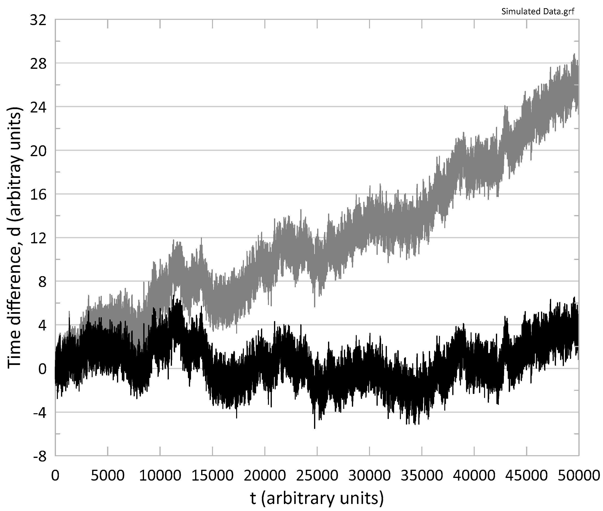
Figure 2.
Noise characteristics of simulated data with drift (solid circles) and without drift (hollow diamonds). TIErms is the time dispersion which quantifies precision and accuracy in time links. ADEVS and TDEV resolve noise types, but ADEVS more accurately characterizes slow noise processes. TDEV is shown only with solid circles since it is the same both with and without drift.
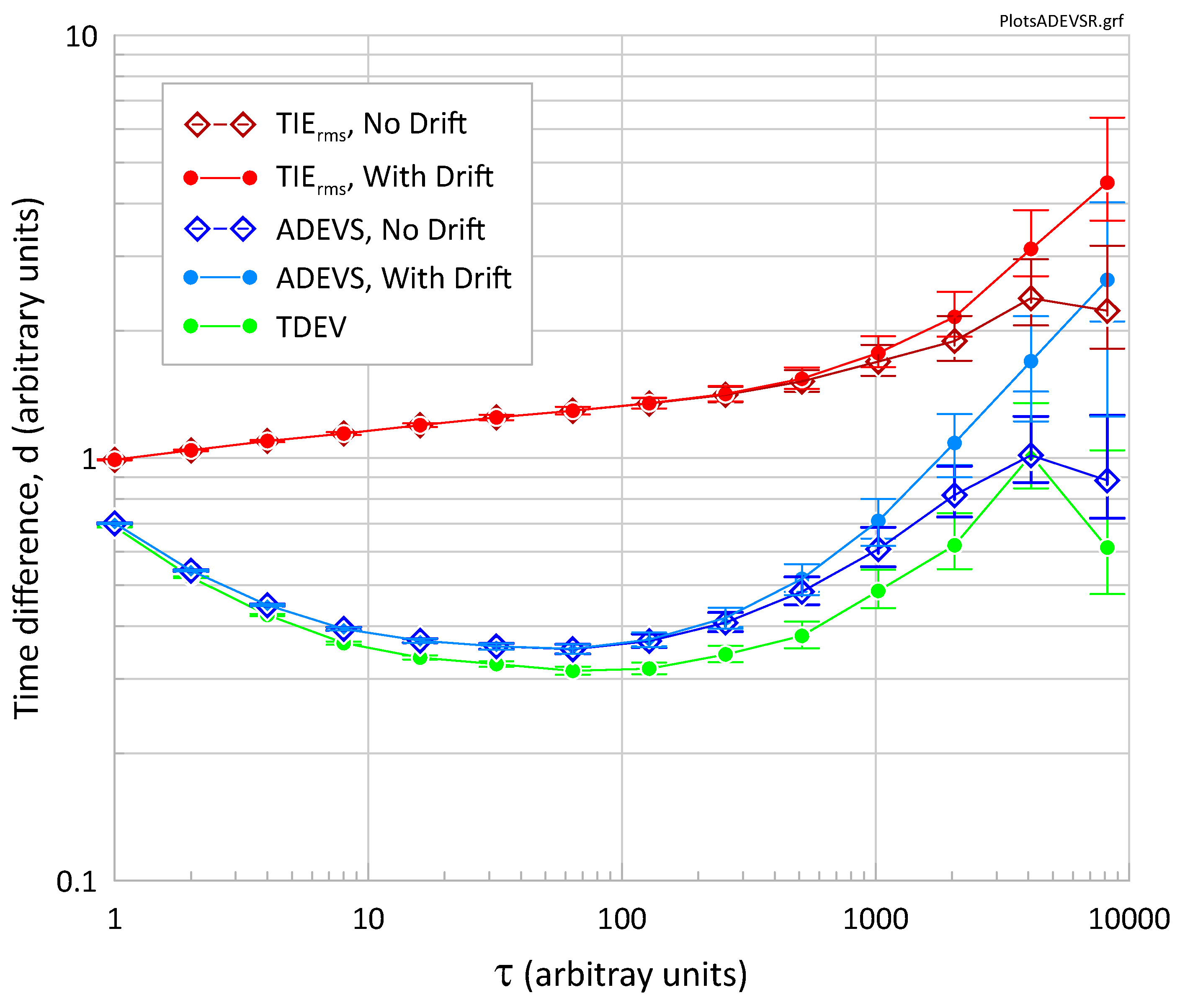
Both TDEV and ADEVS show that the simulated data has the expected noise characteristics. WPN dominates at small τ, and decreases as 1/√τ, FPN dominates at intermediate τ values and is independent of τ, RWPN dominates at large τ, and increases as τ1/2. Both TDEV and ADEVS resolve these characteristics, though TDEV underestimates FPN and RWPN levels. ADEVS is a more direct and accurate measure of slow processes. At large τ the impact of the linear drift is clearly seen. TDEV does not see the drift and therefore gives erroneously small values at large τ. The impact of drift on ADEVS compared to TDEV at τ = 8,192 is more than a factor of 3.
Also note that both TDEV and ADEVS are a poor measure of the time dispersion, TIErms, which is significantly larger [7]. Therefore, TDEV and ADEVS should not be used as estimators for time dispersion or precision. The difference between TIErms and ADEVS at τ = 1 is due to the 1/√2 term in the ADEVS equation. One negative characteristic of TIErms is that it does not resolve the different noise processes very well.
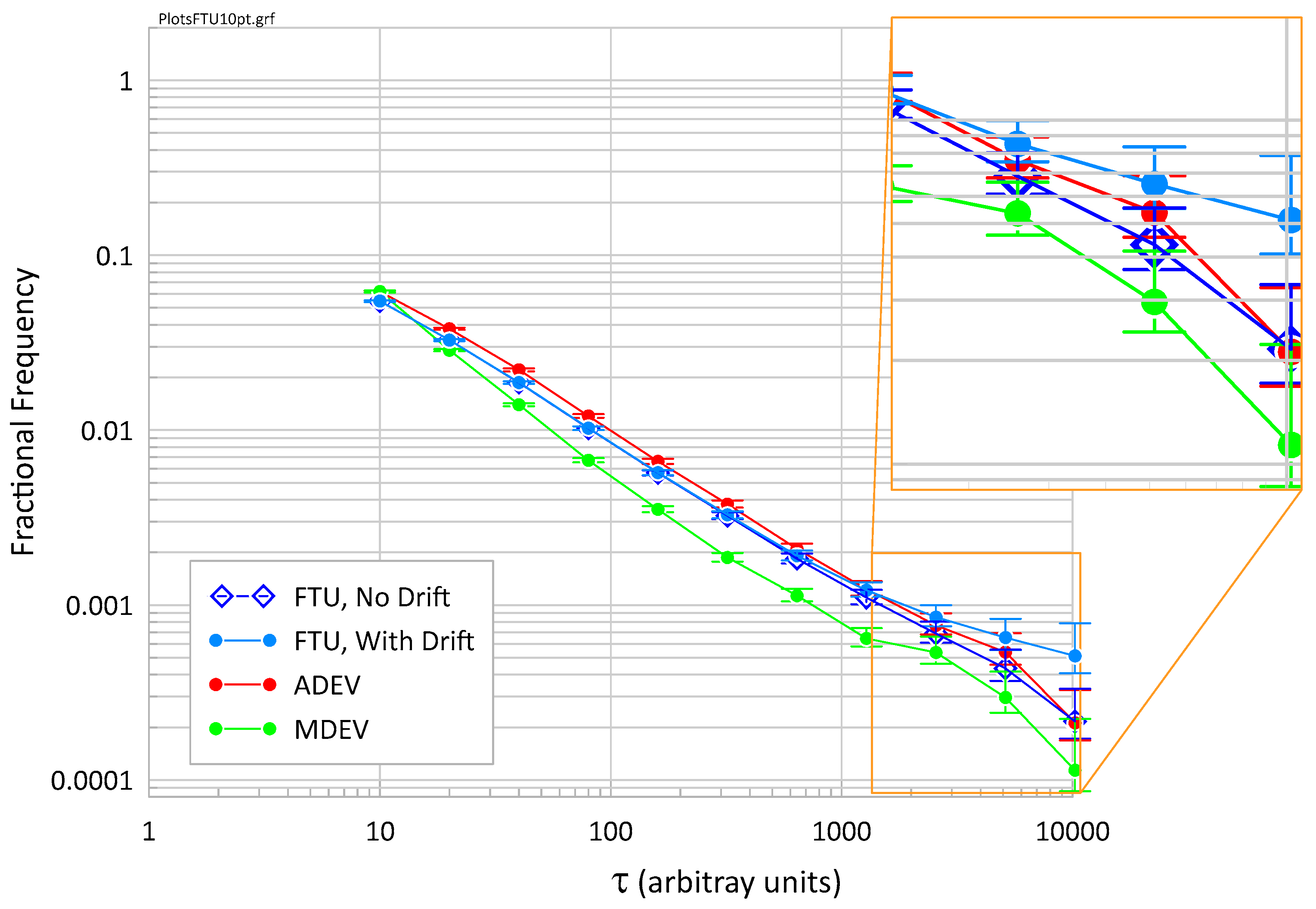
Figure 3 shows the frequency transfer uncertainty, FTU = TIErms/τ, of the simulated data as well as ADEV and MDEV, which are often used to estimate FTU. Again, data with and without drift have been used. As shown in Figure 3, ADEV tends to overestimate the FTU by about 10% to 20% when no drift is present [5]. MDEV significantly underestimates FTU unless the amount of phase averaging in MDEV is taken into accounted [6]. Then the error can be positive or negative depending on the value of τ/τ0, where τ0 is the smallest τ value.
When drift is present, the impact is again greatest at the largest τ values (see the inset). Here, even ADEV may be too low. Though the drift is clearly visible in Figure 1, ADEV is still a passable approximation of the true FTU. Therefore, ADEV can be used as an acceptable (though a little high) estimate of FTU, if there is not an excessive drift in the residual noise. If there is significant linear drift present and ADEV is used, the frequency error introduced by the drift must be included in the frequency uncertainty analysis. However, FTU automatically handles this, as well as higher order drift. MDEV should not be used as an estimator for FTU.
If one is making a frequency comparison and two independent links are present, two values of the frequency difference are obtained. If sufficient information is available about the relative noise levels of the two links a weighted average would be used. However, if this information is not available, the double difference data can be helpful in determining a useful link uncertainty. The double difference is of course the combined noise of the two transfer systems. If an unweighted average of the two frequency difference values is calculated, a useable link uncertainty will be FTU/2 at the appropriate τ value [5]. This may not be the optimum value, but it is the best that can be done with the information available.
In making a phase measurement, the WPN level will be influenced by the measurement hardware bandwidth, specifically the high frequency cutoff, fh. In the presence of WPN, the statistics can be improved with some pre-averaging [15]. For example, the TWSTFT and GPSCP data used by National Metrology Institutes is typically averaged over a few minutes. To illustrate this situation, every 10 points in the data set in Fig 1 have been averaged. Results for TIErms, ADEVS and TDEV are shown in Figure 4 and FTU, ADEV and MDEV in Figure 5. The same vertical and horizontal axes as in Figs. 2 and 3 are used to facilitate comparisons with Figure 4 and Figure 5. TDEV, ADEVS and MDEV are unchanged because they already involve phase averaging, but TIErms, FTU and ADEV are improved.
Averaging of the WPN component significantly reduces the time dispersion and improves precision at all but the largest τ. At τ = 10, the improvement is a factor of 2.1, and at τ = 100, it is 1.7. The same relative improvement is seen in FTU and ADEV in Figure 5. In making a frequency comparison between two standards, averaging down the WPN component of the residual transfer noise will improve the comparison uncertainty.
Averaging is most effective on WPN, but there is also some benefit to averaging FPN. For example, averaging 10 points on pure WPN yields an improvement of 3.16 in TIErms, while the same averaging on pure FPN results in an improvement of only 1.7 at τ = 10. The improvement is even less at larger τ. Averaging RWPN has almost no effect, with only a 16% improvement at τ = 10 and less at larger τ.
5. Summary
Instabilities in transfer systems, commonly called residual noise, can be an important contributor to the total uncertainty in time and frequency comparisons. Second difference statistics such as ADEV, MDEV and TDEV, which were designed for analyzing clock noise, are often used to evaluate these instabilities, but these statistics are not appropriate for use with residual noise. They are not accurate and do not see drift. There are better first difference statistics that should be used. Residual noise can be obtained through techniques such as double differencing or loopbacks. TIErms provides a direct measure of time dispersion in residual noise and is available in Python Allan Tools and Stable 32. TIErms provides important information on the precision and accuracy of time links. Dividing TIErms by τ provides a direct measure of the frequency transfer uncertainty, FTU even in the presence of drift. In the absence of drift, ADEV is a reasonable estimator of FTU, but it is typically 10 to 20% high. When drift is present, it must be included in the frequency transfer uncertainty analysis if ADEV is used. MDEV should not be used because it can easily be misinterpreted and significantly underestimate the transfer uncertainty.
TDEV is often used to investigate the characteristics of residual noise, but ADEVS (easily obtained from ADEV) is a better statistic because it directly sees slow processes and drift. Just like ADEV is an accurate estimator for fractional frequency noise, ADEVS is an accurate estimator for residual phase noise. TDEV under estimates FPN and RWPN. Since ADEVS is easy to use, there is no reason to use TDEV on residual noise. Both TDEV and ADEVS significantly underestimate time dispersion. If WPN is present, some pre-averaging will improve TIErms and FTU. In situations where residual noise is not available, TDEV can be used to characterize transfer noise at short averaging times if the transfer noise is larger than the clock noise.
Funding
This research received no external funding.
Acknowledgments
The author thanks Greg Hoth, Dave Howe, Judah Levine, Biju Patla and Jeff Sherman for helpful discussions.
Conflicts of Interest
The author declares no conflicts of interest.
References
- T. E. Parker, “Invited Review Article: The uncertainty in the realization and dissemination of the SI second from a systems point of view,” Review of Scientific Instruments, 2012, vol. 83 S83, 021102.
- D. W. Allan, “The statistics of atomic frequency standards,” Proc. IEEE, 1966, vol. 54, pp. 221-230.
- D. W. Allan and J.A. Barnes, “A modified Allan variance with increased oscillator characterization ability,” Proc. 35th Freq. Cont. Symp., Philadelphia, PA USA, (27-29 May 1981), pp. 470-474.
- D. W. Allan, M.A. Weiss, and J.L. Jespersen, “A frequency-domain view of time-domain characterization of clocks and time and frequency distribution systems,” Proc. 45th Freq. Cont. Symp., Los Angelas, CA USA, (29-31 May 1991), pp. 667-678.
- G. Panfilo and T. E. Parker, “A theoretical and experimental analysis of frequency transfer uncertainty, including frequency transfer into TAI,” Metrologia, 2010, vol. 47, pp. 552–560.
- T. E. Parker et al., “A three-cornered hat analysis of instabilities in two-way and GPS carrier phase time transfer systems,” Metrologia, 2022, vol. 59, 035007.
- T. E. Parker, R. C. Brown and J. A. Sherman, “Statistics for quantifying aging in time transfer system delays,” Metrologia, 2023, vol. 60, 065011.
- https://github.com/aewallin/allantools.
- W. Riley, 2020 www.stable32.com Stable32 Software.
- D. Kirchner, “Two-Way Satellite Time and Frequency Transfer (TWSTFT): Principle, Implementation, and Current Performance,” Review of Radio Science 1996-1999, Oxford University press, New York, NY USA, 1999, pp. 27-44.
- K. Larson, J. Levine, L. Nelson and T. Parker, “Assessment of GPS Carrier-Phase Stability for Time-Transfer Applications”, IEEE Trans. on Ultrasonics, Ferroelectrics and Frequency Control, 2000, vol. 47, pp. 484-494.
- W. F. McGrew, et. al., “Towards the optical second: verifying optical clocks at the SI limit”, Optica, 2019, vol. 6, pp. 448-454.
- S. Bregni, “Clock Stability Characterization and Measurement in Telecommunications,” IEEE Trans. Instrum. Meas., 1997, vol. 46, pp. 1284-1294.
- D. W. Allan, “Time and Frequency (Time-Domain) Characterization, Estimation, and Prediction of Precision Clocks and Oscillators,” IEEE Trans. on Ultrasonics, Ferroelectrics and Frequency Control, 1987, vol. 34, pp 647-654.
- E. Benkler, C. Lisdat and U. Sterr, “On the relation between uncertainties of weighted frequency averages and the various types of Allan deviations,” Metrologia, 2015, vol. 52, pp. 565–574.
Figure 3.
Frequency transfer uncertainty from the simulated data along with ADEV and MDEV. FTU is the true frequency transfer uncertainty. ADEV and MDEV are only approximations and are the same with and without drift.
Figure 3.
Frequency transfer uncertainty from the simulated data along with ADEV and MDEV. FTU is the true frequency transfer uncertainty. ADEV and MDEV are only approximations and are the same with and without drift.
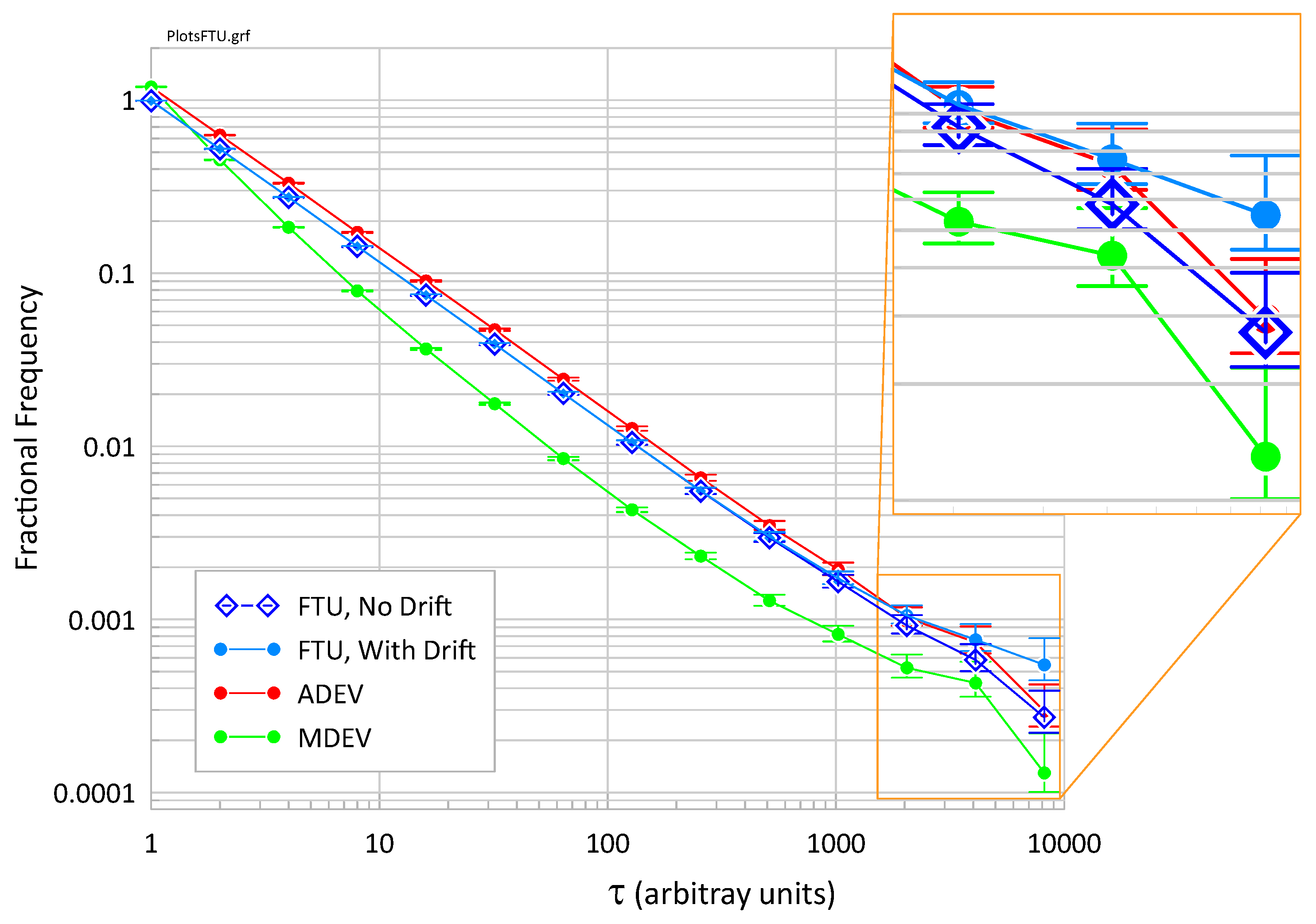
Figure 4.
Noise characteristics of the simulated data with a 10-point average.
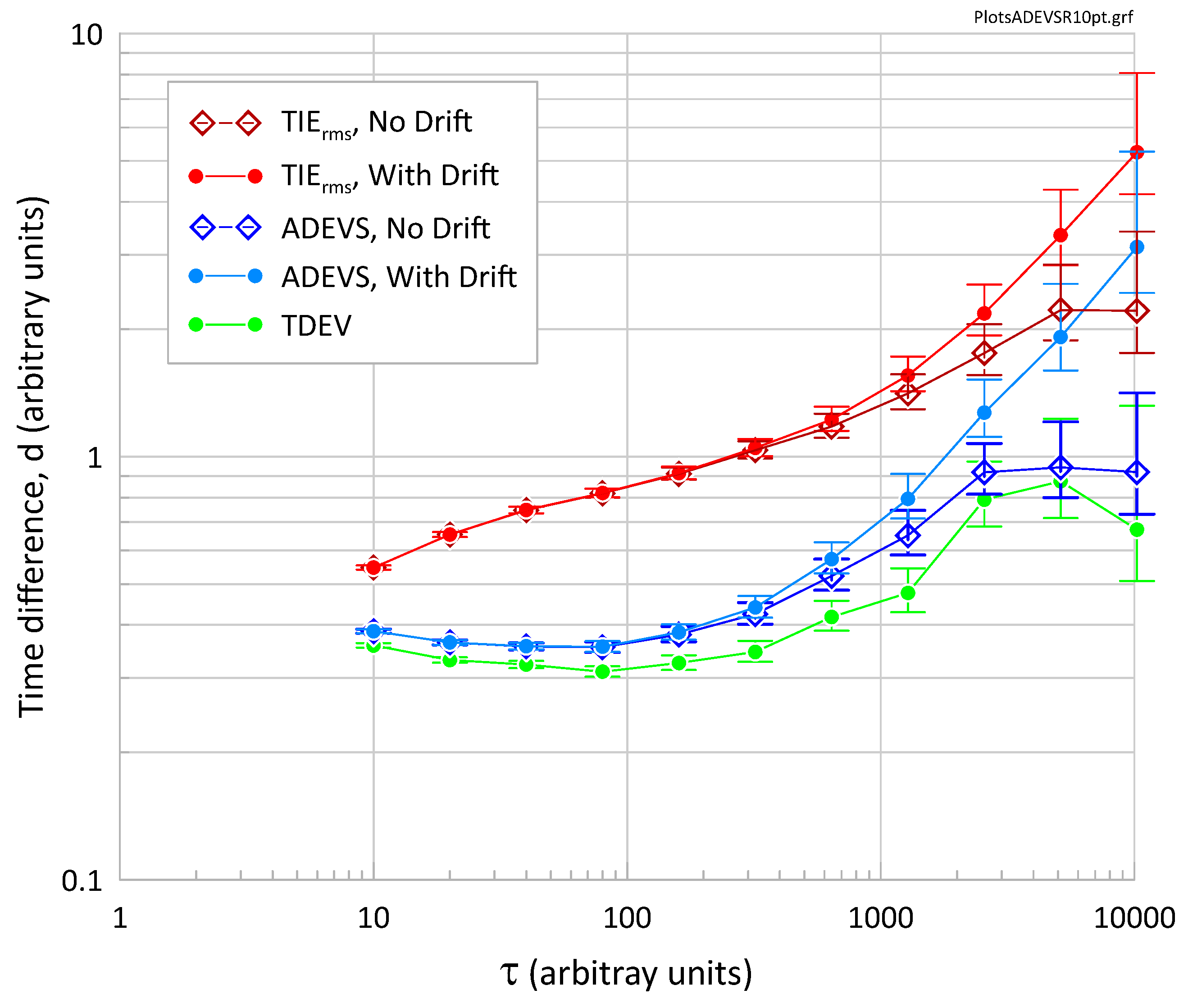
Figure 5.
Frequency transfer uncertainty of the simulated data with a 10-point average.
Disclaimer/Publisher’s Note: The statements, opinions and data contained in all publications are solely those of the individual author(s) and contributor(s) and not of MDPI and/or the editor(s). MDPI and/or the editor(s) disclaim responsibility for any injury to people or property resulting from any ideas, methods, instructions or products referred to in the content. |
© 2025 by the authors. Licensee MDPI, Basel, Switzerland. This article is an open access article distributed under the terms and conditions of the Creative Commons Attribution (CC BY) license (http://creativecommons.org/licenses/by/4.0/).
Copyright: This open access article is published under a Creative Commons CC BY 4.0 license, which permit the free download, distribution, and reuse, provided that the author and preprint are cited in any reuse.


