
Submitted:
30 May 2025
Posted:
30 May 2025
You are already at the latest version
Abstract
Atmospheric turbulence severely degrades high-resolution satellite videos through spatiotemporally coupled distortions, including temporal jitter, spatial-variant blur, deformation, and scintillation, thereby constraining downstream analytical capabilities. Restoring turbulence-corrupted videos poses a challenging ill-posed inverse problem due to the inherent randomness of turbulent fluctuations. While existing turbulence mitigation methods for long-range imaging demonstrate partial success, they exhibit limited generalizability and interpretability in large-scale satellite scenarios. Inspired by refractive-index structure constant (Cn2) estimation from degraded sequences, we propose a physics-informed turbulence signature (TS) prior that explicitly captures spatiotemporal distortion patterns to enhance model transparency. Integrating this prior into a lucky imaging framework, we develop a Physics-Based Turbulence Mitigation Network Guided by Turbulence Signature (TMTS) to disentangle atmospheric disturbances from satellite videos. The framework employs deformable attention modules guided by turbulence signatures to correct geometric distortions, iterative gated mechanisms for temporal alignment stability, and adaptive multi-frame aggregation to address spatially varying blur. Comprehensive experiments on synthetic and real-world turbulence-degraded satellite videos demonstrate TMTS’s superiority, achieving a 0.27 dB PSNR and 0.0015 SSIM improvements over the DATUM baseline while maintaining practical computational efficiency. By bridging turbulence physics with deep learning, our approach provides both performance enhancements and interpretable restoration mechanisms, offering a viable solution for operational satellite video processing under atmospheric disturbances.
Keywords:
turbulence mitigation
; satellite video
; turbulence signature
; atmospheric turbulence
; deep learning
1. Introduction
Satellite video imaging has revolutionized Earth observation by enabling continuous spatiotemporal monitoring of terrestrial dynamics at sub-second temporal resolution and a sub-meter-scale spatial fidelity [1]. This capability supports mission-critical applications such as real-time traffic flow analysis [2], tactical reconnaissance [3], and cross-platform object tracking [4]. A fundamental challenge arises from atmospheric turbulence in the tropospheric boundary layer, which introduces spatiotemporally correlated distortions during image acquisition. As illustrated in Figure 1, the degradation originates from turbulence-induced wavefront phase disturbances, driven by vertically stratified profiles with horizontal anisotropy along the line-of-sight atmospheric path. As these disturbances propagate, they lead to intensity distribution dispersion, peak intensity reduction, and positional displacement at the focal plane. Consequently, satellite videos exhibit temporal jitter, random blurring, and geometric distortion. Such visual degradation compromises target clarity and obscures morphological details, thereby leading to performance drops of subsequent applications. Effective turbulence mitigation is therefore a prerequisite for operational satellite video analytics.
Compared with adaptive optics systems [5,6] that require sophisticated wavefront correctors and real-time controllers, turbulence mitigation (TM) algorithms offer a computationally efficient solution to this ill-posed inverse problem. Conventional TM methodologies predominantly employ lucky imaging frameworks, which statistically select and fuse minimally distorted frames. Law et al. [7] pioneered this paradigm in ground-based visible-light imaging by developing quality-aware frame selection metrics. Subsequent innovations include Joshi et al.’s [8] locally-adaptive lucky-region fusion to suppress blurring artifacts and Anantrasirichai’s [9] dual-tree complex wavelet transform approach for spatial distortion correction. Mao et al. [10] further advanced the field through spatiotemporal non-local fusion, achieving hybrid photometric-geometric compensation. However, these methods suffer from limited robustness under strong turbulence and dynamic conditions, often yielding suboptimal restoration results due to mismatches between real-world turbulent imaging environments and idealized assumptions. Furthermore, their computationally intensive optimization frameworks frequently lead to performance degradation in practical deployments.
Recent breakthroughs in deep learning, particularly its demonstrated efficacy in low-level vision tasks, have established data-driven TM as the state-of-the-art approach for restoring degraded imagery [11,12,13]. Supervised learning frameworks utilizing paired turbulence-distorted/clean datasets currently dominate TM research, benefiting from their capacity to model deterministic degradation processes. Transformer architectures have emerged as powerful tools for single-frame TM task. Mao et al. [14] pioneered a spatial-adaptive processing network that captures long-range dependencies to address turbulence-induced distortions. Complementary work by Li et al. [15] demonstrated that U-Net structures with global feature aggregation can effectively mitigate atmospheric distortions in remote sensing applications. However, such single-frame methods inherently fail to resolve geometric distortions, as temporal information loss in isolated frames prevents complete turbulence parameter estimation. To overcome this limitation, multi-frame TM frameworks have been developed to exploit spatiotemporal correlations across sequential observations. By aggregating high-frequency details from multiple degraded frames, these methods achieve superior reconstruction fidelity. Terrestrial imaging systems have particularly benefited from such approaches. A turbulence-specific Wasserstein GAN framework [16] that inverts degradation processes via adversarial learning. Zou et al. [17] integrates deformable 3D convolutions with Swin transformers to handle motion artifacts in long-range videos. Zhang et al. [18] combines deformable attention with temporal-channel mechanisms, enabling pixel-level registration through lucky imaging principles. Despite terrestrial successes, existing multi-frame TM methods face satellite limitations due to altitude-varying turbulence, orbital dynamics, missing physics integration, and absent physics regularization for unseen regimes.
Physics-based methods provide a compelling alternative for TM task by explicitly modeling atmospheric degradation mechanisms. The systematic integration of turbulence-governed physical processes, particularly phase distortion modeling [19], spatiotemporal point spread function (PSF) variations [10], and physical parameters of the turbulence field [20], have demonstrated substantial benefits. These approaches not only yield more accurate and reliable results but also improve the generalization capability across varying turbulence conditions. The parameter, a fundamental metric for atmospheric turbulence quantification, has been successfully integrated into collaborative learning frameworks for joint artifact suppression and turbulence estimation in thermal infrared imagery [20]. However, satellite-based TM implementation faces two unresolved challenges. First, the requirement for synchronized two-dimensional turbulence field measurements, typically acquired through ground-based scintillometer networks, conflicts with orbital platforms’ inherent lack of in-situ sensing capabilities. Second, while recent studies [21,22,23] propose video-based estimation methods leveraging temporal intensity correlations, their functional integration with TM tasks remains experimentally unverified under orbital imaging conditions characterized by rapid platform motion and variable observation geometries.
The classical model [21,22] for estimating 2D fields from distorted video distinguishes two variable categories: video-intrinsic features (image gradients, temporal intensity variance) and imaging-system parameters (pixel field-of-view, imaging distance, optical aperture diameter). Satellite TM tasks exhibit unique advantages through homologous video sequences sharing identical imaging-system parameters, allowing these parameters to be treated as constants. Under this constraint, we define turbulence signature-a physics - informed metric calculated from gradient-temporal analysis - to quantify scaled spatial distributions. As demonstrated in Fig. Figure 2, turbulence signature provides three critical functionalities: (1) enhanced distortion feature visualization in raw video frames , (2) sparse representation enabling efficient large-scale inference, and (3) strong positive correlation with distortion severity. This discovery motivates our turbulence signature-guided modeling strategy, which resolves the limitation of conventional TM methods, namely their incapacity to incorporate turbulence physics as inductive bias, via explicit feature encoding.
Specifically, this study proposes a physics-based Turbulence Mitigation network guided by Turbulence Signature (TMTS) for satellite video. The turbulence signature models spatiotemporal distortions through direct extraction image gradients and local temporal intensity variance from the source video, thereby eliminating external data dependencies. Maintaining model interpretability through the three-stage framework of feature alignment, reference reconstruction, and temporal fusion, the architecture incorporates three novel modules: Turbulence Signature Guided Alignment (TSGA), Convolutional Gated Reference Feature Update (CGRFU), and Turbulence-Spatial-Temporal Self-Attention (TSTSA). By integrating turbulence signatures, these modules concentrate on effective distortion information, substantially constraining solution space complexity. The TSGA module leverages deformation attention on downsampled deep features to activate global geometric distortion representations, replacing conventional optical flow methods with physics-aware compensation. The CGRFU module addresses misalignment propagation via convolutional gating mechanisms that model long-range temporal dependencies in reference features. The TSTSA module enhances complementary feature aggregation in low-distortion regions via adaptive attention mechanisms.
In brief, our contributions are listed as follows. (1) Physics-Informed Turbulence Signature: A spatiotemporal distortion prior constructed directly from raw video provides explicit physical constraints without requiring external instrumentation. This approach improves generalizability across varying atmospheric conditions. (2) Task-Specific Network Modules: Three turbulence signature-integrated components target critical aspects. TSGA module enables global geometric compensation for turbulence-distorted features, while CGRFU module ensures dynamically reliable reference construction. TSTSA module further accomplishes adaptive fusion of spatiotemporally complementary information. (3) Synergistic Framework: Tightly integrates physical priors with deep learning through turbulence signature-guided three-stage TM processing, enhancing the interpretability of network models with minimal complexity growth. (4) Cross-Platform Validation: Comprehensive evaluations across five satellite systems (Jilin-1, Carbon-2, UrtheCast, Skysat-1, and Luojia3-01) demonstrate state-of-the-art performance.
2. Proposed Method
2.1. Turbulence Signature
The proposed turbulence signature is derived from estimating the refractive index structure constant using consecutive image sequences. To provide a clearer understanding of this process, we first briefly review the classical approach to estimating . Higher values indicate stronger turbulence, causing stronger wavefront distortions. The retrieval of relies on statistical analysis of angle of arrival (AOA) variance [21]. When video-based remote sensing systems operating in the inertial subrange (), the monoaxial AOA variance for unbounded plane waves is expressed in radians as:
where denotes the angular variance component (rad) of AOA fluctuations, D is the aperture diameter, represents the optical wavelength, L corresponds to the propagation path length, while and characterize the inner scale and outer scale of atmospheric turbulence, respectively. A wavefront angular shift of radians at the optical aperture induces a lateral image displacement of pixels, where is the pixel field of view. Consequently, the single-axis variance of the image displacement caused by AOA fluctuations can be mathematically expressed as:
This conversion bridges wavefront-level turbulence () to pixel-level displacement (), enabling video-based quantification. Note that since the AOA variance is equal in all axes, it is appropriate to specify the image offset variance along each axis, X and Y , represented by . Turbulence disrupts temporal image sampling, creating nonuniform spatial discretization. To quantify turbulence-induced spatial discretization, we derive the temporal intensity variance as:
where and are the vertical and the horizontal derivatives of the ideal image at point , respectively. Given that the local intensity temporal variance and the derivatives and can be calculated from the consecutive image sequence, the explicit formulation of the retrieval may be systematically derived through
Equation (4) reveals two key insights: (1) Satellite parameters , D, and L remain constant; (2) depends on spatiotemporal features . This mathematical framework enables quantitative identification of turbulence strength at arbitrary pixel coordinates across temporal frames. The magnitude of S directly correlates with local turbulence intensity, serving as a probabilistic indicator of turbulence-induced distortion likelihood. Formally, we define this spatiotemporally resolved metric as the turbulence signature (TS). As demonstrated in Figure 2, TS captured in the Jilin-1 and Carbonite-2 satellite videos reveal significant correlations between spatial-temporal degradation patterns and optical turbulence effects. These degradation patterns, which manifest through space-variant blur and geometric distortion, collectively facilitate the spatiotemporal mapping of atmospheric refractive index fluctuations. This empirical evidence motivates us to develop an enhanced restoration framework for turbulence-degraded satellite video by integrating a physically interpretable turbulence signature into the reconstruction process.
2.2. TMTS Network
2.2.1. Overview
Given a continuous sequence of frames from a satellite video that captures atmospheric turbulence degradation, denoted as , where represents the target frame for reconstruction, while the remaining frames are its adjacent counterparts. The goal of our network is to reconstruct satellite video frames that mitigate turbulence effects, ensuring that the reconstruction results closely approximate . Figure 3 illustrates the overall structure of the proposed method, which utilises the DATUM recursive network structure [18]. This structure comprises three stages: features alignment, lucky fusion, and post-processing.
Features Alignment Stage: For each input frame at time t, residual dense blocks (RDB) perform downsampling operations. These blocks facilitate the extraction of three levels of features while concurrently capturing turbulence signature . We propose an alignment module informed by turbulence signature, TSGA, to align deep features with the preceding hidden state . The CGRFU module effectively models spatiotemporal features of turbulent degradation, incorporating long-range dependencies and recursively updating the hidden reference feature .
Lucky Fusion Stage: The aligned features and hidden state are integrated using a series of RDB to produce the forward embedding . This embedding is presumed to remain unaffected by turbulence, allowing for the update of the hidden reference feature r. Following the bidirectional recursive process, the novel self-attention module, TSTSA, is introduced for the effective fusion of feature layers. This module processes forward embedding , backward embedding , and bidirectional embedding of adjacent frames, along with fusion features derived from TS.
Post-processing Stage: Features obtained from lucky fusion are decoded into turbulence-free satellite video frames. A dual decoder design is implemented. One decoder generates a compensation field for turbulent geometric distortion, which is used to alert the clear image of geometric distortion and to compute the loss of geometric structure restoration with . The other decoder reconstructs the clear video frame free from turbulence distortion.
2.2.2. TSGA Module for Feature Alignment
In contrast to natural and turbulence-free satellite videos, turbulence-degraded satellite videos exhibit not only moving subjects of varying scales but also significant random geometric distortions induced by turbulence [1,24]. Therefore, capturing motion information and compensating for chaotic geometric distortions become more complex. Conventional deformation convolution-based techniques [25,26] are incapable of learning intricate enclosed turbulent geometric distortion motion information due to their restricted receptive field. Consequently, we introduce a TSGA module that utilizes turbulence signatures as a priori to direct the deep feature alignment of the image. The turbulence signature incorporates the spatial location and the relative intensity of the relationship between the geometric distortions caused by turbulence in each frame of the satellite video, as implicitly described by the input frame sequence. This prior can incorporate global spatio-temporal information for aberration compensation for each distinct frame, rather than solely relying on local temporal information between adjacent frames, such as optical flow.
The objective of our TSGA module is to synchronize feature with prospective reference features to enhance the utilization of the spatiotemporal information inherent in the turbulence signature for modeling completion. We utilize SpyNet [27] estimation of optical flow to derive a coarse deformation field, to which warping is applied for initial feature alignment. The turbulence signature is input into a convolutional layer and activated by a sigmoid function. This activated signature is then linked to the aligned features, hidden reference features, and deformation field, while displacement offsets are predicted by a residual dense block. The GDA module utilizes offsets that have experienced several iterations of multiclustered deformation attentions to align the input features with the hidden features . This procedure is articulated as:
Among them, [·] represents the connection operation, denotes the warping operation, and the sigmoid function is indicated . represents the turbulence signature, denotes the aligned feature, and signifies the updated deformation field from feature to reference.
2.2.3. CGRFU Module for Reference Feature Update
Feature alignment requires the participation of reference features, as previously discussed [28,29]. However, the presence of atmospheric turbulence complicates the construction of reference features derived from local temporal characteristics, due to the randomness of geometric deformations in satellite videos. To address this, we introduce the CGRFU module. This module effectively captures long-distance temporal dependencies and constructs more precise reference features by considering the global time information conveyed by TS and the Gaussian-like, multi-frame jitter characteristics [30] of turbulent degraded satellite videos. The core idea is to integrate convolution operations and the turbulence signature into the Gated Recurrent Unit (GRU). This allows the concurrent collection of spatial characteristics and temporal dependence of reference features. By concealing information from the preceding moment to the present, together with a gated mechanism, the module adaptively acquires significant aspects for the construction of reference features.
Structurally, the CGRFU module closely mirrors the GRU, incorporating update gates, reset gates, and hidden states. The pivotal distinction lies in the module’s tripartite input: the turbulence signature, the hidden state from the preceding time step and the forward embedding. The turbulence signature, which encapsulates the spatial and temporal characteristics of atmospheric turbulence, is initially processed through a convolutional layer followed by a sigmoid activation function. This processed signature is then concatenated with the forward embedding residual, forming an augmented feature tensor. Subsequently, this tensor is partitioned into reset and update gates via a gating mechanism. The reset gate and update gate regulate the extent to which the current hidden state retains or discards information from the preceding hidden state. This adaptive gating process enables the CGRFU module to dynamically capture long-range temporal dependencies and construct more precise reference features, thereby enhancing the robustness of feature alignment in the presence of turbulent distortions. The update gate U and reset gate G indicate the proportion of the current time step’s hidden state r used to retain and discard information from the preceding time step:
where denotes the tensor partitioning operation. r indicates the hidden state from the previous time step, and Z refers to the residual connection between the turbulence signature activated by the sigmoid function and the forward embedding:
To enhance the capture of temporal dependencies within the sequence, the turbulence signature S, forward embedding e, and the prior hidden state r, processed by the reset gate G, are integrated to produce a new candidate hidden state. This integration is achieved through nonlinear activation using the function.
Subsequently, the candidate hidden states are weighted and fused with the hidden states from the previous time step via the update gate , resulting in the hidden state for the current time step.
The update gate assesses the influence of the prior hidden state and the candidate hidden states on the current hidden state. The CGRFU module performs recursive updates to the hidden feature , which serves as a reference for correcting turbulent geometric distortions.
2.2.4. TSTSA for Lucky Fusion
Although the deep features of adjacent consecutive frames have been aligned, it remains crucial to integrate their complementary information. To address this, we design TSTSA module. This module processes the bidirectional embedding and TS from the current frame and its adjacent frames as input. It generates a feature tensor that encapsulates the complementary characteristics of consecutive frames. Bidirectional embedding ensures uniform restoration quality across various frames. The participation of TS aims to enhance the lucky fusion process by directing focus towards spatial regions with more pronounced turbulence signature. This approach facilitates the model’s ability to learn key features more efficiently and enhances its generalization capabilities. These insights stem from a fundamental analysis indicating that the blurriness associated with turbulence is typically observed in areas characterized by higher turbulence signature values. While aligned bidirectional embedding features present challenges in assessing the extent of blur distortion, TS offers a practical and empirical benchmark.
The TSTSA module begins by concatenating the channels from multiple frames and then reduces the channel dimension using convolution. Separable convolution is employed to construct spatially varying queries, keys, and values across both temporal and channel dimensions. The turbulence signature, generated via convolution and a sigmoid function, is used to compute the attention score through dot multiplication with the query-key product. The attention score is normalized using the Softmax function to produce attention weights. These weights are applied to aggregate the value vectors, forming the attention map.
Here, denotes the softmax operation applied along the row direction of Q. Q, K, and V represent the query, key, and value matrices derived from the concatenated multi temporal channel features. These features pass through linear transformations via a GELU activation layer and a convolutional layer, respectively. C represents the scaling factors. denotes the turbulence signature after sigmoid activation.
2.2.5. Loss Fuction
A composite loss function is developed that integrates pixel level fidelity loss and geometric distortion loss , represented by the following formula:
We empirically set , . is engineered to achieve high fidelity at the pixel level. To quantify the pixel-level differences between the model output and the reference image, we utilised the Charbonnier loss function [31]. This function provides a balance between robustness to outliers and the preservation of high-frequency detail information in the reconstruction results:
where denotes the restored image, while signifies the target reference image. is a small constant. is implemented to eliminate geometric distortions induced by turbulence in the reconstruction processing. One of the dual decoders is utilized to estimate the inverse tilt field. Subsequently, the image containing only the tilt is warped to assess its difference from the reference image.
where T represents the inverse tilt field estimated by the decoder, while denotes the image that exclusively contains tilt without blurring, which can be produced in turbulent degraded satellite video sequences.
3. Experiment and Discussion
3.1. Satellite Video Datasource
Our turbulence mitigation framework was evaluated using video data from five prominent video satellite platforms: Jilin-1 (primary data source), Carbonite-2, UrtheCast, Skysat-1, and Luojia3-01. The training dataset comprised 189 non-overlapping 512×512 patches curated from Jilin-1 sequences, following the methodology of [1]. For benchmark evaluation, we stratified test data across platforms: five scenes from two distinct Jilin-1 videos, four scenes each from Carbonite-2 and UrtheCast, three from Skysat-1, and two from Luojia3-01. Each 100-frame temporal sequence preserves spatiotemporal turbulence characteristics. The final dataset contains 189 training clips and 18 test scenes across five satellites, with detailed specifications in Table 1.
3.2. Paired Turbulence Data Synthesis
Our framework employs an autoregressive model [32] as an efficient atmospheric turbulence simulator, synthesizing paired turbulence data through Taylor’s frozen flow hypothesis and temporal phase screen theory. Given that atmospheric turbulence within 20 km altitude predominantly affects Earth observation satellites, we model light propagation from ground targets as spherical wavefronts traversing conical turbulence volumes prior to spaceborne sensor acquisition.
As show in Figure 4, the simulation adopts a multi-layer turbulence integration approach [33], stratifying atmospheric disturbances into three vertically distributed phase screens (1 km, 4 km, and 20 km altitudes) with respective weighting coefficients of 0.6, 0.3, and 0.1. Wind-driven temporal dynamics are controlled via velocity parameters (≤5 m/s) governing turbulent structure advection, thereby generating spatiotemporally correlated distortions. Satellite imaging geometry is constrained to 400-600 km orbital ranges, with atmospheric coherence lengths calibrated between 3-10 cm using Hufnagel-Valley profile models [34]. Post-simulation processing introduces Gaussian noise () to emulate sensor noise characteristics.
3.3. Implementation Details
The computational framework was implemented in PyTorch on a workstation with an AMD EPYC 9754 CPU and NVIDIA RTX 4090 GPU. Our architecture employs a three-layer convolutional encoder (16 kernels/layer) preceding TSGA module, which incorporates 8 parallel deformable attention groups. Training configuration utilized 240×240 pixel inputs with batch size 2 over 1000 epochs, optimized via Adam [40] (, ) and cosine annealing scheduling (). All network parameters were jointly optimized through backpropagation.
3.4. Metrics
The quantitative evaluation of atmospheric turbulence mitigation efficacy in our framework employs three principal metrics. For synthetic dataset validation, established image quality benchmarks including the Peak Signal-to-Noise Ratio (PSNR) and Structural Similarity Index (SSIM) are utilized to quantify reconstruction fidelity relative to ground truth references. In real-world applications where reference images are unavailable, three no-reference metrics were employed: 1) Blind/Referenceless Image Spatial Quality Evaluator (BRISQUE) [41] analyzes statistical features of locally normalized luminance coefficients to detect distortions in natural scene statistics; 2) Contrast Enhancement-based Image Quality (CEIQ) [42] evaluates degradation by quantifying pixel intensity distribution changes during contrast enhancement processes; 3) Natural Image Quality Evaluator (NIQE) [43] measures the distance between statistical features of restored images and a multivariate Gaussian model derived from pristine natural scenes. Notably, lower BRISQUE and NIQE scores indicate superior perceptual quality aligned with human visual assessment criteria.
3.5. Performance on Synthetic Datasets
We compared the proposed TSTM with six state-of-the-art models specifically designed for turbulence mitigation tasks on synthetic datas: TSRWGAN [16], NDIR [35], TMT [37], DeturNet [15], TurbNet [14] and DATUM [18]. Additionally, four state-of-the-art generic video restoration models were included in the comparison: VRT [38], RVRT [29], x-Restormer [39], and Shift-net [36].To enable impartial evaluation, all models were retrained on our synthetic datasets. PSNR and SSIM were adopted as objective metrics to evaluate the fidelity of restoration results. It should be noted that both PSNR and SSIM calculations were performed in the YCbCr color space to align with human visual perception characteristics.
3.5.1. Quantitative Evaluation
Table 2, Table 3 and Table 4 provide quantitative comparisons in terms of PSNR and SSIM across five satellite video datasets, demonstrating the performance of benchmark models in 18 distinct operational scenarios. Our empirical observations reveal that generic video restoration models yield only marginal improvements compared with specialized turbulence mitigation architectures. This performance discrepancy primarily originates from the inherent spatiotemporal distortions characteristic of turbulence-degraded videos - particularly atmospheric-induced non-uniform geometric warping and temporally varying blur patterns - which fundamentally challenge the generalizability of conventional restoration paradigms to satellite-based turbulence mitigation tasks. Notably, the proposed TMTS framework demonstrates superior efficacy over competing methods, achieving significant performance gains across all satellite video benchmarks. This consistent superiority suggests TMTS maintains robust reconstruction capabilities under varying imaging configurations and diverse remote sensing scenarios. Specifically, compared with the state-of-the-art DATUM model, our TMTS exhibits a 0.27 dB average PSNR improvement. This enhancement quantitatively validates our method’s capacity to exploit turbulence-specific spatiotemporal signatures for deriving relative atmospheric turbulence intensity metrics, thereby enabling physics-aware restoration of remote sensing video sequences.
3.5.2. Qualitative Results
The subjective restoration results of seven video satellite turbulence-degraded synthetic sequences are illustrated in Figure 5, Figure 6 and Figure 7. Our method demonstrates superior visual clarity and structural fidelity, with restored geometric features closely aligned with ground truth while effectively mitigating turbulence-induced distortions. In magnified patches, our model achieves enhanced reconstruction of fine details, including alphanumeric characters, architectural components, and regional boundaries. Specifically, in scene-2 of Jilin-1, the runway numbers reconstructed by VRT, RVRT, and X-Restormer exhibit excessive blurring, rendering them indistinguishable. This highlights the limitations of generic video restoration models in preserving temporal details under turbulence degradation. In Scene 7 of Carbonite-2, TurbNet, TSRWGAN, and TMT retain spatially-varying blur artifacts in the terminal roof region, particularly distorting the circular truss structures. In Scene 11 of UrtheCast, while TMTS successfully maintains the shape and edges of circular markers on buildings, competing methods lacking iterative reference frame reconstruction (e.g., VRT, RVRT, X-Restormer) fail to recover severely warped structural edges. TurbNet, TSRWGAN, and TMT further introduce edge blurring and artifacts. Though DATUM achieves relative accuracy, its results remain less sharp compared to TMTS.
As shown in Figure 5, TMTS reconstructs crisp linear features of buildings and partially restores spiral textures on surfaces. All competing methods except DATUM and TMTS yield distorted edges despite recovering coarse structures. Figure 6 presents magnified details from two Luojia3-01 satellite scenes, where TMTS demonstrates superior high-frequency detail restoration compared to other approaches. The visual comparisons confirm that our physics-based module, which incorporates temporal averaging information and adaptively responds to localized turbulence-induced deformations, achieves structurally faithful reference frame construction. This mechanism enables targeted compensation of high-frequency features into degraded frames through adaptive fusion, thereby achieving significant perceptual improvements over state-of-the-art baselines.
3.6. Performance on Real Data
To validate the effectiveness of the proposed TMTS in addressing real-world degradation in satellite video, experiments were conducted on the SatSOT dataset [44]. Notably, this dataset contains no simulated degradations, with testing exclusively performed on image sequences exhibiting visually confirmed significant atmospheric turbulence degradation.
Table 5 presents the turbulence mitigation performance of various methods in terms of BRISQUE, CEIQ, and NIQE metrics. The results demonstrate that TMTS achieves the best performance in BRISQUE and NIQE, while ranking second in CEIQ, indicating its strong robustness and competitiveness in addressing turbulence mitigation challenges for real-degraded remote sensing images. Significantly, the optimal BRISQUE and NIQE scores highlight TMTS’s superiority in restoring human perception-aligned authentic results. Furthermore, the high CEIQ score confirms the capability of our TMTS to effectively reconstruct high-frequency textures in complex real-world scenarios affected by turbulence degradation.
Figure 8 provides a visual comparison of turbulence mitigation in real-world remote sensing videos. Observations reveal that our TMTS effectively corrects localized geometric distortions and generates visually appealing textures with rich high-frequency details. Specifically, the red and yellow regions of interest (ROIs) illustrate that TMTS produces sharper and more distinct edges, thereby delivering visually superior outcomes. These findings validate the efficacy of TMTS in addressing turbulence mitigation tasks for satellite videos, demonstrating its practical utility in real-world applications.
To systematically evaluate the temporal coherence and consistency of turbulence mitigation methods, a row of pixels was recorded and temporally stacked to generate corresponding y-t temporal profiles. As illustrated in Figure 9, our TMTS produces more precise and smoother long-term temporal details, highlighting the effectiveness of turbulence signature in suppressing turbulence-induced temporal jitter.
3.7. Ablation Studies
Our ablation framework systematically evaluates critical architectural determinants that introduce effective inductive biases into the model architecture, including turbulence signature modeling, multi-stage architectural integration of turbulence signature operators, temporal sequence length optimization, and window-based feature aggregation mechanisms. The experimental protocol further extends to encompass quantitative assessments of computational budget and operational efficiency.
3.7.1. Effect of Turbulence Signature
To advance computational efficiency and improve interpretability in deep learning frameworks for satellite video turbulence mitigation, we propose turbulence signature encoding to explicitly model multi-scale distortion characteristics inherent in atmospheric turbulence degradation. Validation experiments employing benchmark evaluations under identical training protocols demonstrate that architectures integrating turbulence signature operators outperform their ablated counterparts by statistically significant margins. Qualitative comparisons in Figure Figure 10 visually confirm the signature’s capacity to spatially resolve turbulence-induced artifacts, effectively distinguishing between space-variant blur patterns and geometric deformation regions. This discriminative capability enables deep networks to adaptively prioritize distortion correction in critical areas, thus achieving enhanced turbulence suppression fidelity while maintaining computational tractability.
3.7.2. Effect of TSGA, CGRFU and TSTSA
This study systematically validates the functional efficacy of individual architectural components within the TMTS framework through a multi-stage ablation protocol. The foundational architecture employs TSTSA module that strategically aggregates spatiotemporal embeddings from adjacent frames via window-based feature fusion. All comparative analyses were conducted under strictly controlled experimental conditions, maintaining identical training configurations and evaluation metrics. The component-level ablation investigation focuses on three core modules: TSGA, CGRFU, and TSTSA. Through component-wise deactivation experiments, we progressively removed turbulence signature operators (denoted as w/o configurations) from each module to quantify their performance contributions. Experimental results (Table 6) quantitatively establish the differential contributions of TSGA, CGRFU, and TSTSA modules to turbulence suppression efficacy, revealing that integrated operation of all components achieves optimal distortion rectification through complementary feature refinement mechanisms.
TSGA module addresses registration challenges of turbulence-induced non-rigid geometric distortions by leveraging turbulence signature encoding as a physics-aware prior for deep feature alignment. As quantified in Table 5, integration of TSGA enhances reconstruction fidelity compared to baseline architectures, achieving PSNR/SSIM improvements of +1.64 dB and +0.0318 respectively. This performance gap highlights the criticality of explicit spatiotemporal distortion modeling for atmospheric turbulence degradation.
The CGRFU module introduces convolutional operations and turbulence signature encoding into gated recurrent architectures, enabling synergistic integration of spatial characteristics and temporal dependencies in reference feature refinement. This novel architectural innovation establishes turbulence-resilient reference features through adaptive spatiotemporal filtering, effectively suppressing atmospheric distortion propagation across sequential frames. Experimental comparisons demonstrate that incorporating CGRFU yields measurable performance enhancements, with quantitative metrics improving by +1.07 dB PSNR and +0.0095 SSIM. This empirically demonstrates the critical role of dynamic reference feature updating in achieving robust temporal alignment for satellite video sequences under turbulent conditions.
Notably, the removal of TS operator from the TSGA module demonstrates only minimal performance improvements, thereby highlighting the critical importance of the proposed encoding mechanism for effective turbulence mitigation. This observed performance discrepancy primarily stems from the distinctive capability of turbulence signatures to resolve distortion patterns specifically induced by atmospheric turbulence through the integration of refractive-index-aware spatial constraints. The framework achieves enhanced distortion characterization by embedding physics-derived calculations of atmospheric refractive-index structure parameters ( values), which facilitate precise identification of turbulence-induced geometric deformation patterns. Specifically, this approach enables comprehensive spatial mapping of distortion concentration regions and quantitative analysis of localized intensity variations, consequently reducing feature misregistration errors during geometric transformation processes through optimized deformation field estimation.
3.7.3. Influence of Input Frame Number
In turbulence mitigation tasks, the frame quantity employed during both training and inference phases critically determines reconstruction outcomes. Given that turbulence-induced degradation originates from zero-mean random phase distortions, enhanced frame perception enables the network to theoretically achieve more precise estimation of turbulence-free states through spatiotemporal analysis. This principle remains valid for quasi-static remote sensing scenarios characterized by limited moving targets, where pixel-level turbulence statistics demonstrate enhanced temporal tractability for systematic tracking and analytical processing.
Three models were developed using 10-, 20-, and 30-frame input sequences, with their comparative performance metrics across varying inference-phase frame conditions systematically analyzed in Figure 11. Experimental results demonstrate a statistically significant positive correlation between turbulence mitigation efficacy and input sequence length under temporal acquisition constraints inherent to remote sensing video systems. Specifically, incremental increases in frame quantity generate performance improvements exceeding 1dB in objective metrics. These findings confirm that effective turbulence mitigation in remote sensing video processing requires temporal integration of scene information across prolonged frame sequences, a computational principle directly analogous to the multi-frame fusion strategies used in remote sensing video super-resolution tasks.
3.7.4. Model Efficiency and Computation Budget
To rigorously evaluate model efficiency, we conducted a comprehensive analysis of the correlations among FLOPs, parameter counts, and PSNR metrics, as visualized in Figure 12(a). The reported PSNR values represent averages calculated across 18 distinct scenes from five satellite video sequences. Our model demonstrates superior computational efficiency by occupying the optimal upper-left quadrant in the parametric space analysis, indicating enhanced restoration performance (higher PSNR values on the y-axis) coupled with reduced computational complexity (lower FLOPs on the x-axis) and compact model size.
Further computational analysis, presented in Figure 12(b), compares inference time budgets across competing architectures under standardized testing conditions using a single NVIDIA 4090 GPU. Our framework achieves state-of-the-art processing efficiency with a turbulence mitigation latency of approximately 0.19 seconds per image. While this performance currently falls short of real-time processing requirements, it significantly outperforms existing benchmark methods in terms of inference speed while maintaining competitive restoration quality.
3.8. Limitations and Future Works
While the proposed TMTS model demonstrates superior performance across multiple aspects of turbulence mitigation in remote sensing video processing, several limitations warrant further investigation:
(1) Constructing Ground-Truth Turbulence Datasets
The staring imaging technology employed by remote sensing satellites enables sustained observation of designated target areas, capturing dynamic variations and generating continuous image sequences. Post-acquisition orbital adjustments facilitate revisit capabilities for re-imaging identical geographical regions, creating opportunities to acquire temporally aligned video pairs containing turbulence-degraded and turbulence-free observations of the same scenes. Such datasets provide objective quantitative benchmarks for evaluating turbulence mitigation algorithms, enabling precise modeling of degradation-restoration mappings under supervised learning frameworks. This approach effectively constrains model optimization trajectories while enhancing the physical consistency and visual fidelity of restoration outcomes.
(2) Exploring TS Potential
The turbulence signature mechanism, inspired by values estimation methodologies, leverages gradient features and global variance statistics from current frames. This approach demonstrates operational validity in staring imaging scenarios where static backgrounds dominate remote sensing observations. However, the global per-pixel variance computation exhibits inherent limitations when handling multi-scale moving targets and satellite attitude variations. Dynamic objects and orbital coverage changes introduce motion artifacts distinct from turbulence distortions, causing TS in these regions to encapsulate coupled multi-dimensional interference. Current methodology insufficiently addresses the interplay between moving targets, attitude dynamics, and turbulence signatures, potentially compromising reconstruction fidelity. To address these constraints, future investigations should prioritize developing dedicated feature extraction protocols for moving targets through integration of average optical flow estimation and unsupervised motion segmentation [45], which enables decoupling of dynamic/static scene components prior to turbulence correction, while concurrently establishing explicit mathematical relationships between turbulence signatures and phase distortion mechanisms inherent to atmospheric turbulence effects to enhance the physical interpretability of restoration frameworks.
4. Conclusions
This study proposes a physics-based turbulence mitigation network guided by turbulence signature (TMTS) for satellite video processing, designed to overcome critical limitations inherent in existing purely deep learning-based approaches. Drawing inspiration from image sequence-derived estimation methodologies, we develop a turbulence signature extraction mechanism that directly derives spatiotemporal distortion priors from raw video gradients and localized temporal intensity variance, thereby eliminating external dataset dependencies for physics-guided networks. The turbulence signature is systematically integrated into three computational modules under a lucky imaging paradigm: the TSGA module employs signature-driven priors to achieve robust geometric compensation through deformation-aware alignment of deep features; the CGRFU module leverages turbulence signatures carrying global temporal statistics to model long-range dependencies of quasi-Gaussian jitter patterns across multi-frame satellite videos, enabling precise reference feature construction; and the TSTSA module enhances inter-frame interactions by adaptively fusing complementary features in weakly distorted regions through signature-informed attention mechanisms.
To evaluate TMTS’s efficacy, comparative experiments are conducted on five satellite video datasets (Jilin-1, Carbon-2, UrtheCast, Skysat-1, Luojia3-01), with turbulence-degraded sequences synthesized using temporal phase screens and autoregressive models. Our model demonstrates superior performance against six specialized turbulence mitigation models and four general video restoration frameworks, achieving average improvements of 0.27 dB (PSNR) and 0.0015 (SSIM) on synthetic data, while reducing non-reference metrics NIQE and BRISQUE by 4.05 % and 4.46 % on real-world data. Subjective evaluations and temporal profile analyses confirm TMTS’s generalization capability in complex remote sensing scenarios. Systematic ablation studies validate the necessity of physics-informed inductive biases, particularly the turbulence signature’s role in enhancing spatiotemporal distortion characterization.
By explicitly encoding turbulence signatures into its architecture, TMTS effectively disentangles spatiotemporal geometric distortions and blur artifacts, producing visually coherent reconstructions with enhanced interpretability for operational satellite applications. The framework establishes a critical bridge between turbulence physics and deep learning, demonstrating that physics-driven inductive biases significantly improve model generalizability.
Author Contributions
Conceptualization, J.Y. and T.S.; methodology, J.Y. and G.Z.; software, J.Y. and X.Z.; validation, J.Y., J.H. and X.Z.; formal analysis, J.Y. and X.Z; investigation, J.Y. and T.S.; resources, J.Y. and X.W.; data curation, J.Y.,T.S.,G.Z. and X.Z.; writing—original draft preparation, J.Y.; writing—review and editing, J.Y. and T.S.; visualization, J.Y., X.Z. and T.S.; supervision, J.Y.; project administration, J.Y.; funding acquisition, T.S. All authors have read and agreed to the published version of the manuscript.
Funding
This research was funded by the National Key Research and Development Project of China (NO. 2020YFF0304902) and the Hubei Key Research and Development (NO. 2021BAA201).
Data Availability Statement
Our dataset are available at https://github.com/whuluojia (accessed on 1 March 2025).
Conflicts of Interest
The authors declare no conflicts of interest.
References
- Xiao, Y.; Yuan, Q.; Jiang, K.; Jin, X.; He, J.; Zhang, L.; Lin, C.W. Local-Global Temporal Difference Learning for Satellite Video Super-Resolution. IEEE Trans. Circuits Syst. Video Technol. 2024, 34, 2789–2802. [Google Scholar] [CrossRef]
- Zhao, B.; Han, P.; Li, X. Vehicle Perception From Satellite. IEEE Transactions on Pattern Analysis and Machine Intelligence 2024, 46, 2545–2554. [Google Scholar] [CrossRef]
- Han, W.; Chen, J.; Wang, L.; Feng, R.; Li, F.; Wu, L.; Tian, T.; Yan, J. Methods for Small, Weak Object Detection in Optical High-Resolution Remote Sensing Images: A survey of advances and challenges. IEEE Geosci. Remote Sens. Mag. 2021, 9, 8–34. [Google Scholar] [CrossRef]
- Zhang, Z.; Wang, C.; Song, J.; Xu, Y. Object Tracking Based on Satellite Videos: A Literature Review. Remote Sens. 2022, 14. [Google Scholar] [CrossRef]
- Rigaut, F.; Neichel, B. Multiconjugate Adaptive Optics for Astronomy. In ANNUAL REVIEW OF ASTRONOMY AND ASTROPHYSICS, VOL 56; Faber, S.; VanDishoeck, E., Eds.; 2018; Vol. 56, Annual Review of Astronomy and Astrophysics, pp. 277–314. [CrossRef]
- Liang, J.; Williams, D.; Miller, D. Supernormal vision and high-resolution retinal imaging through adaptive optics. J. Opt. Soc. Am. A 1997, 14, 2884–2892. [Google Scholar] [CrossRef]
- Law, N.; Mackay, C.; Baldwin, J. Lucky imaging: high angular resolution imaging in the visible from the ground. Astron. Astrophys. 2006, 446, 739–745. [Google Scholar] [CrossRef]
- Joshi, N.; Cohen, M. Seeing Mt. Rainier: Lucky Imaging for Multi-Image Denoising, Sharpening, and Haze Removal. In Proceedings of the 2010 IEEE International Conference on Computational Photography (ICCP 2010). IEEE, 2010 2010, p. 8 pp. 2010 IEEE International Conference on Computational Photography (ICCP 2010), 29-30 March 2010, Cambridge, MA, USA.
- Anantrasirichai, N.; Achim, A.; Kingsbury, N.G.; Bull, D.R. Atmospheric Turbulence Mitigation Using Complex Wavelet-Based Fusion. IEEE Trans. Image Process. 2013, 22, 2398–2408. [Google Scholar] [CrossRef]
- Mao, Z.; Chimitt, N.; Chan, S.H. Image Reconstruction of Static and Dynamic Scenes Through Anisoplanatic Turbulence. IEEE Trans. Comput. Imaging 2020, 6, 1415–1428. [Google Scholar] [CrossRef]
- Cheng, J.; Zhu, W.; Li, J.; Xu, G.; Chen, X.; Yao, C. Restoration of Atmospheric Turbulence-Degraded Short-Exposure Image Based on Convolution Neural Network. Photonics 2023, 10. [Google Scholar] [CrossRef]
- Ettedgui, B.; Yitzhaky, Y. Atmospheric Turbulence Degraded Video Restoration with Recurrent GAN (ATVR-GAN). Sensors 2023, 23. [Google Scholar] [CrossRef]
- Wu, Y.; Cheng, K.; Cao, T.; Zhao, D.; Li, J. Semi-supervised correction model for turbulence-distorted images. Opt. Express 2024, 32, 21160–21174. [Google Scholar] [CrossRef] [PubMed]
- Mao, Z.; Jaiswal, A.; Wang, Z.; Chan, S.H. Single Frame Atmospheric Turbulence Mitigation: A Benchmark Study and a New Physics-Inspired Transformer Model. In Proceedings of the COMPUTER VISION, ECCV 2022, PT XIX; Avidan, S.; Brostow, G.; Cisse, M.; Farinella, G.; Hassner, T., Eds., 2022, Vol. 13679, Lecture Notes in Computer Science, pp. 430–446. 17th European Conference on Computer Vision (ECCV), Tel Aviv, ISRAEL, OCT 23-27, 2022. [CrossRef]
- Li, X.; Liu, X.; Wei, W.; Zhong, X.; Ma, H.; Chu, J. A DeturNet-Based Method for Recovering Images Degraded by Atmospheric Turbulence. Remote Sens. 2023, 15. [Google Scholar] [CrossRef]
- Jin, D.; Chen, Y.; Lu, Y.; Chen, J.; Wang, P.; Liu, Z.; Guo, S.; Bai, X. Neutralizing the impact of atmospheric turbulence on complex scene imaging via deep learning. Nat. Mach. Intell. 2021, 3, 876–884. [Google Scholar] [CrossRef]
- Zou, Z.; Anantrasirichai, N. DeTurb: Atmospheric Turbulence Mitigation with Deformable 3D Convolutions and 3D Swin Transformers. In Proceedings of the Computer Vision - ACCV 2024: 17th Asian Conference on Computer Vision, Proceedings. Lecture Notes in Computer Science (15475); Cho, M.; Laptev, I.; Tran, D.; Yao, A.; Zha, H., Eds., 2025 2025, pp. 20–37. Asian Conference on Computer Vision, 2024, Hanoi, Vietnam. [CrossRef]
- Zhang, X.; Chimitt, N.; Chi, Y.; Mao, Z.; Chan, S.H. Spatio-Temporal Turbulence Mitigation: A Translational Perspective. In Proceedings of the 2024 IEEE/CVF CONFERENCE ON COMPUTER VISION AND PATTERN RECOGNITION, CVPR 2024. IEEE; IEEE Comp Soc; CVF, 2024, IEEE Conference on Computer Vision and Pattern Recognition, pp. 2889–2899. IEEE/CVF Conference on Computer Vision and Pattern Recognition (CVPR), Seattle, WA, JUN 16-22, 2024. [CrossRef]
- WANG, J.; MARKEY, J. MODAL COMPENSATION OF ATMOSPHERIC-TURBULENCE PHASE-DISTORTION. J. Opt. Soc. Am. 1978, 68, 78–87. [Google Scholar] [CrossRef]
- Wang, Y.; Jin, D.; Chen, J.; Bai, X. Revelation of hidden 2D atmospheric turbulence strength fields from turbulence effects in infrared imaging. Nat. Comput. Sci. 2023, 3, 687–699. [Google Scholar] [CrossRef]
- Zamek, S.; Yitzhaky, Y. Turbulence strength estimation from an arbitrary set of atmospherically degraded images. J. Opt. Soc. Am. A 2006, 23, 3106–3113. [Google Scholar] [CrossRef]
- Saha, R.K.; Salcin, E.; Kim, J.; Smith, J.; Jayasuriya, S. Turbulence strength Cn2 estimation from video using physics-based deep learning. Opt. Express 2022, 30, 40854–40870. [Google Scholar] [CrossRef]
- Beason, M.; Potvin, G.; Sprung, D.; McCrae, J.; Gladysz, S. Comparative analysis of Cn2 estimation methods for sonic anemometer data. Appl. Opt. 2024, 63, E94–E106. [Google Scholar] [CrossRef]
- Zeng, T.; Shen, Q.; Cao, Y.; Guan, J.Y.; Lian, M.Z.; Han, J.J.; Hou, L.; Lu, J.; Peng, X.X.; Li, M.; et al. Measurement of atmospheric non-reciprocity effects for satellite-based two-way time-frequency transfer. Photon. Res. 2024, 12, 1274–1282. [Google Scholar] [CrossRef]
- Zhang, Y.; Sun, Y.; Liu, S. Deformable and residual convolutional network for image super-resolution. Appl. Intell. 2022, 52, 295–304. [Google Scholar] [CrossRef]
- Luo, G.; Qu, J.; Zhang, L.; Fang, X.; Zhang, Y.; Man, S. Variational Learning of Convolutional Neural Networks with Stochastic Deformable Kernels. In Proceedings of the 2022 IEEE International Conference on Systems, Man, and Cybernetics (SMC), 2022 2022, pp. 1026–31. 2022 IEEE International Conference on Systems, Man, and Cybernetics (SMC), 9-12 Oct. 2022, Prague, Czech Republic. [CrossRef]
- Ranjan, A.; Black, M.J. Optical Flow Estimation using a Spatial Pyramid Network. In Proceedings of the 30TH IEEE CONFERENCE ON COMPUTER VISION AND PATTERN RECOGNITION (CVPR 2017). IEEE; IEEE Comp Soc; CVF, 2017, IEEE Conference on Computer Vision and Pattern Recognition, pp. 2720–2729. 30th IEEE/CVF Conference on Computer Vision and Pattern Recognition (CVPR), Honolulu, HI, JUL 21-26, 2017. [CrossRef]
- Rucci, M.A.; Hardie, R.C.; Martin, R.K.; Gladysz, S.Z.Y.M.O.N. Atmospheric optical turbulence mitigation using iterative image registration and least squares lucky look fusion. Appl. Opt. 2022, 61, 8233–8247. [Google Scholar] [CrossRef] [PubMed]
- Liang, J.; Fan, Y.; Xiang, X.; Ranjan, R.; Ilg, E.; Green, S.; Cao, J.; Zhang, K.; Timofte, R.; Van Gool, L. Recurrent Video Restoration Transformer with Guided Deformable Attention. In Proceedings of the ADVANCES IN NEURAL INFORMATION PROCESSING SYSTEMS 35 (NEURIPS 2022); Koyejo, S.; Mohamed, S.; Agarwal, A.; Belgrave, D.; Cho, K.; Oh, A., Eds., 2022, Advances in Neural Information Processing Systems. 36th Conference on Neural Information Processing Systems (NeurIPS), ELECTR NETWORK, NOV 28-DEC 09, 2022. [CrossRef]
- Lau, C.P.; Lai, Y.H.; Lui, L.M. Restoration of atmospheric turbulence-distorted images via RPCA and quasiconformal maps. Inverse Probl. 2019, 35. [Google Scholar] [CrossRef]
- Barron, J. A General and Adaptive Robust Loss Function. In Proceedings of the 2019 IEEE/CVF Conference on Computer Vision and Pattern Recognition (CVPR). Proceedings, 2019 2019, pp. 4326–34. 2019 IEEE/CVF Conference on Computer Vision and Pattern Recognition (CVPR), 15-20 June 2019, Long Beach, CA, USA. [CrossRef]
- Srinath, S.; Poyneer, L.A.; Rudy, A.R.; Ammons, S.M. Computationally efficient autoregressive method for generating phase screens with frozen flow and turbulence in optical simulations. Optics Express 2015, 23, 33335–33349. [Google Scholar] [CrossRef]
- Chimitt, N.; Chan, S.H. Simulating Anisoplanatic Turbulence by Sampling Correlated Zernike Coefficients. In Proceedings of the 2020 IEEE International Conference on Computational Photography (ICCP); 2020; pp. 1–12. [Google Scholar] [CrossRef]
- Wu, X.Q.; Yang, Q.K.; Huang, H.H.; Qing, C.; Hu, X.D.; Wang, Y.J. Study of Cn2 profile model by atmospheric optical turbulence model. Acta Phys. Sin. 2023, 72. [Google Scholar] [CrossRef]
- Li, N.; Thapa, S.; Whyte, C.; Reed, A.; Jayasuriya, S.; Ye, J. Unsupervised Non-Rigid Image Distortion Removal via Grid Deformation. In Proceedings of the 2021 IEEE/CVF INTERNATIONAL CONFERENCE ON COMPUTER VISION (ICCV 2021). IEEE; CVF; IEEE Comp Soc, 2021, pp. 2502–2512. 18th IEEE/CVF International Conference on Computer Vision (ICCV), ELECTR NETWORK, OCT 11-17, 2021. [CrossRef]
- Li, D.; Shi, X.; Zhang, Y.; Cheung, K.C.; See, S.; Wang, X.; Qin, H.; Li, H. A Simple Baseline for Video Restoration with Grouped Spatial-temporal Shift. In Proceedings of the 2023 IEEE/CVF CONFERENCE ON COMPUTER VISION AND PATTERN RECOGNITION (CVPR). IEEE; CVF; IEEE Comp Soc, 2023, IEEE Conference on Computer Vision and Pattern Recognition, pp. 9822–9832. IEEE/CVF Conference on Computer Vision and Pattern Recognition (CVPR), Vancouver, CANADA, JUN 17-24, 2023. [CrossRef]
- Zhang, X.; Mao, Z.; Chimitt, N.; Chan, S.H. Imaging Through the Atmosphere Using Turbulence Mitigation Transformer. IEEE Trans. Comput. Imaging 2024, 10, 115–128. [Google Scholar] [CrossRef]
- Liang, J.; Cao, J.; Fan, Y.; Zhang, K.; Ranjan, R.; Li, Y.; Timofte, R.; Van Gool, L. VRT: A Video Restoration Transformer. IEEE Trans. Image Process. 2024, 33, 2171–2182. [Google Scholar] [CrossRef] [PubMed]
- Chen, X.; Li, Z.; Pu, Y.; Liu, Y.; Zhou, J.; Qiao, Y.; Dong, C. A Comparative Study of Image Restoration Networks for General Backbone Network Design. In Proceedings of the COMPUTER VISION - ECCV 2024, PT LXXI; Leonardis, A.; Ricci, E.; Roth, S.; Russakovsky, O.; Sattler, T.; Varol, G., Eds. AIM Group, 2025, Vol. 15129, Lecture Notes in Computer Science, pp. 74–91. 18th European Conference on Computer Vision (ECCV), Milan, ITALY, SEP 29-OCT 04, 2024. [CrossRef]
- Diederik, P.; Kingma, J.B. Adam: A Method for Stochastic Optimization. In Proceedings of the In Proceedings of the International Conference on Learning Representations (ICLR), 2015 2015, pp. 1–15. [CrossRef]
- Mittal, A.; Moorthy, A.K.; Bovik, A.C. No-Reference Image Quality Assessment in the Spatial Domain. IEEE Trans. Image Process. 2012, 21, 4695–4708. [Google Scholar] [CrossRef] [PubMed]
- Fang, Y.; Ma, K.; Wang, Z.; Lin, W.; Fang, Z.; Zhai, G. No-Reference Quality Assessment of Contrast-Distorted Images Based on Natural Scene Statistics. IEEE Signal Processing Letters 2015, 22, 838–842. [Google Scholar] [CrossRef]
- Mittal, A.; Soundararajan, R.; Bovik, A.C. Making a “Completely Blind” Image Quality Analyzer. IEEE Signal Process. Lett. 2013, 20, 209–212. [Google Scholar] [CrossRef]
- Li, S.; Zhou, Z.; Zhao, M.; Yang, J.; Guo, W.; Lv, Y.; Kou, L.; Wang, H.; Gu, Y. A Multitask Benchmark Dataset for Satellite Video: Object Detection, Tracking, and Segmentation. IEEE Trans. Geosci. Remote Sens. 2023, 61. [Google Scholar] [CrossRef]
- Saha, R.K.; Qin, D.; Li, N.; Ye, J.; Jayasuriya, S. Turb-Seg-Res: A Segment-then-Restore Pipeline for Dynamic Videos with Atmospheric Turbulence. In Proceedings of the 2024 IEEE/CVF CONFERENCE ON COMPUTER VISION AND PATTERN RECOGNITION (CVPR). IEEE; IEEE Comp Soc; CVF, 2024, IEEE Conference on Computer Vision and Pattern Recognition, pp. 25286–25296. IEEE/CVF Conference on Computer Vision and Pattern Recognition (CVPR), Seattle, WA, JUN 16-22, 2024. [CrossRef]
Figure 1.
Schematic diagram of distortion in satellite video caused by atmospheric turbulence. (a) Satellite video imaging geometry highlighting tropospheric turbulence-induced optical wavefront distortions. (b) Degraded video frames exhibiting geometric displacement, space-varient blur, and temporal jitter.
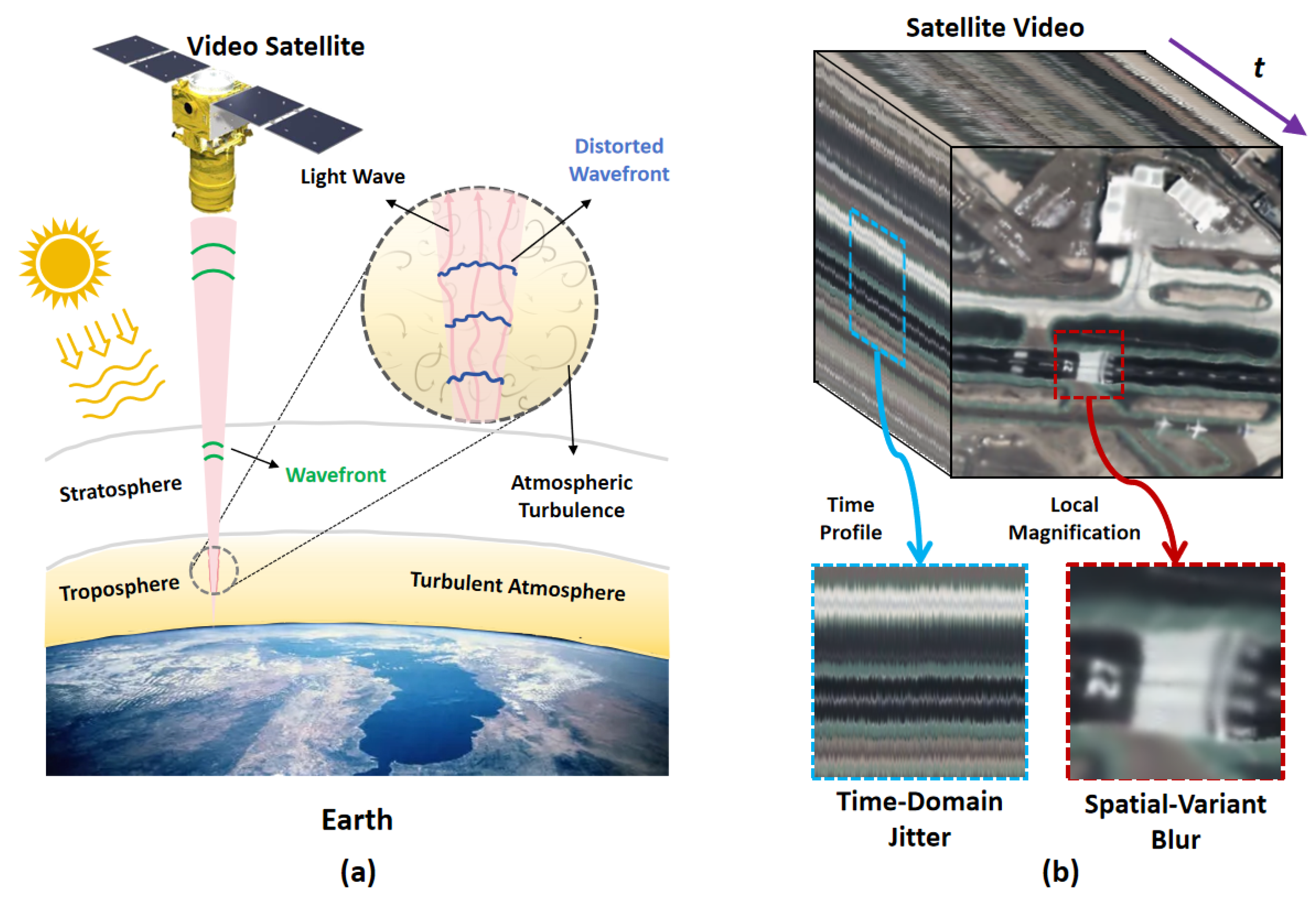
Figure 2.
Turbulence signature observed in satellite video frames. Turbulence signature is produced through physics-based estimation techniques [21,22], revealing clues of relative turbulence intensity across various spatial positions and temporal instances in satellite videos.
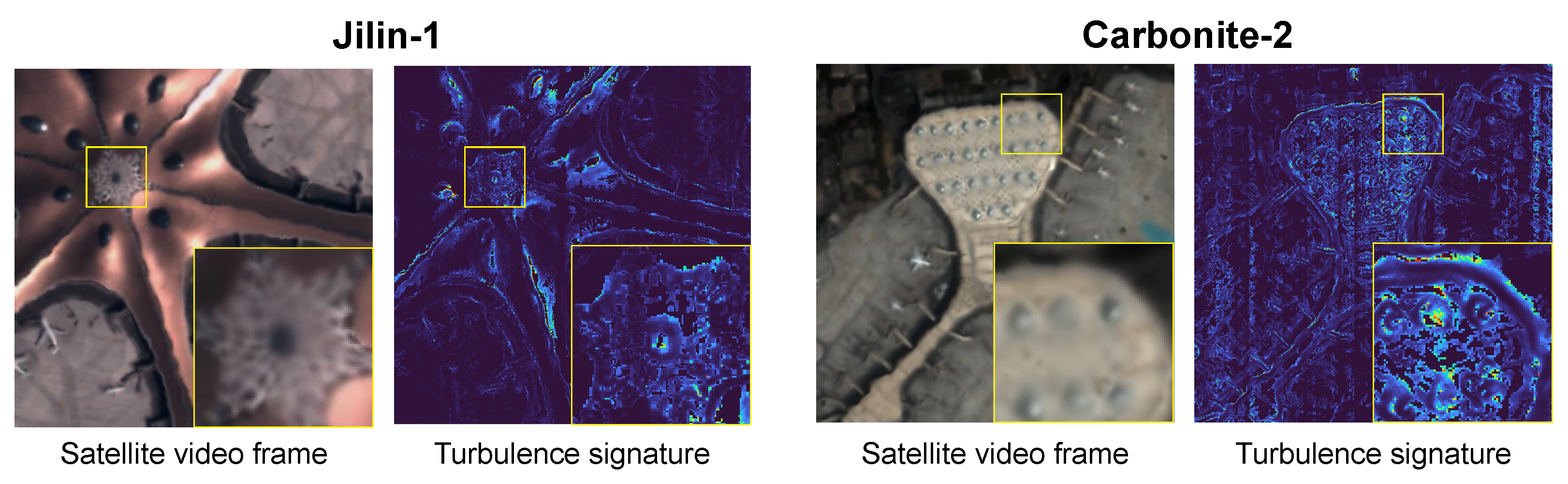
Figure 3.
The overall architecture of our proposed TMTS network. It comprises three modules: (1) Turbulence Signature Guided Alignment (TSGA) module for deep feature alignment; (2) Convolutional Gated Reference Feature Update (CGRFU) module for reference feature update; (3) Turbulent Spatiotemporal Self-Attention (TSTSA) module for the aggregation of multi-channel spatiotemporal feature information.
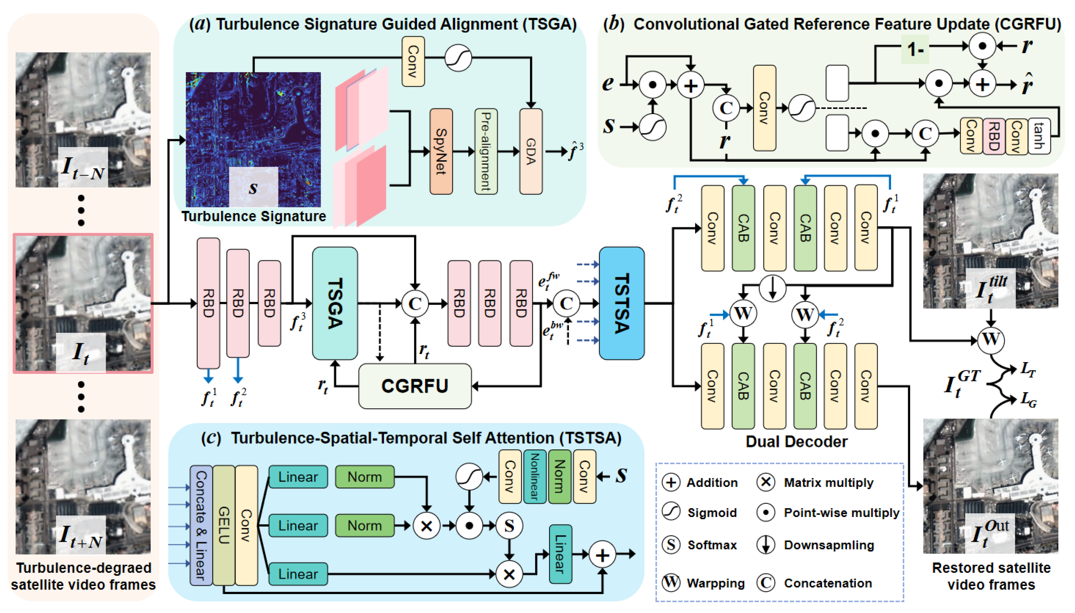
Figure 4.
Stratified turbulence simulation for satellite imaging. (a) Altitude-dependent phase perturbations; (b) Original vs. simulated turbulence-degraded Images.
Figure 4.
Stratified turbulence simulation for satellite imaging. (a) Altitude-dependent phase perturbations; (b) Original vs. simulated turbulence-degraded Images.
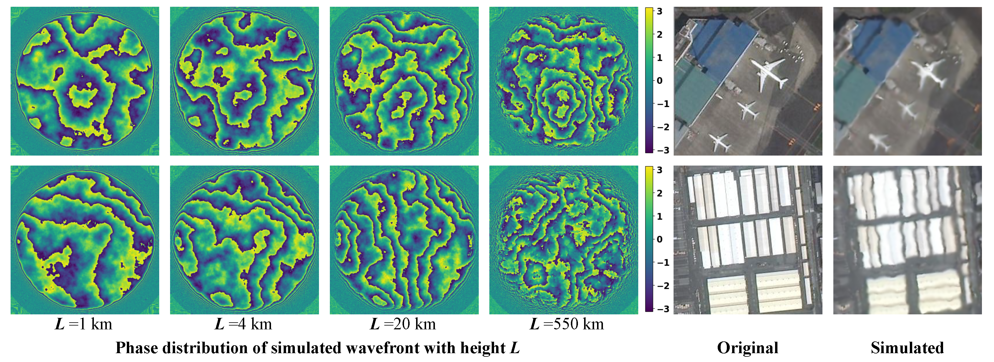
Figure 5.
Qualitative comparisons on scene-2 of Jilin-1, scene-7 of Carbonite-2, and scene-11 from UrtheCast. Zoom in for better visualization.
Figure 5.
Qualitative comparisons on scene-2 of Jilin-1, scene-7 of Carbonite-2, and scene-11 from UrtheCast. Zoom in for better visualization.
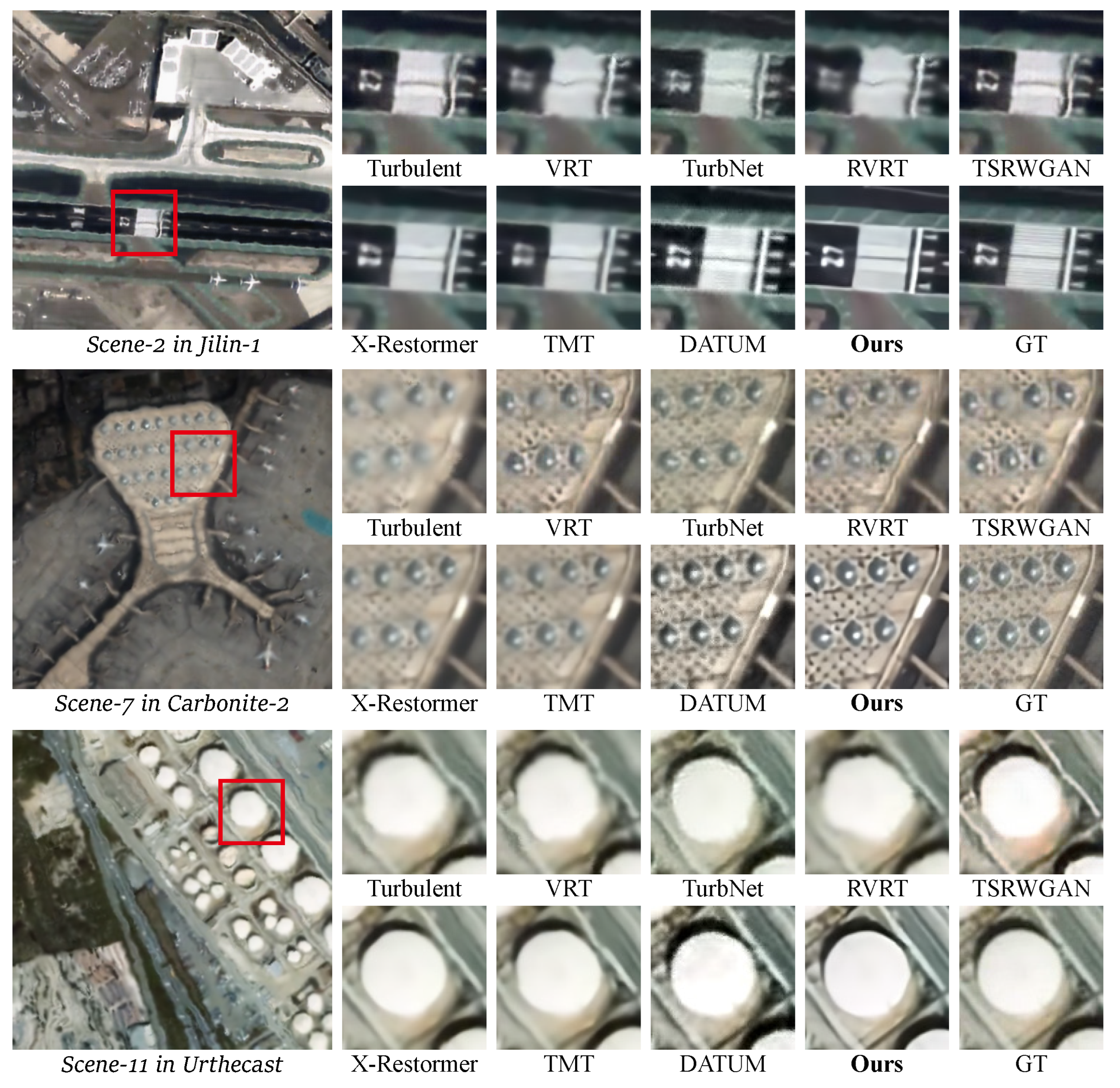
Figure 6.
Qualitative comparisons on scene-14 and scene-15 of SkySat-1. Zoom in for better visualization.
Figure 6.
Qualitative comparisons on scene-14 and scene-15 of SkySat-1. Zoom in for better visualization.
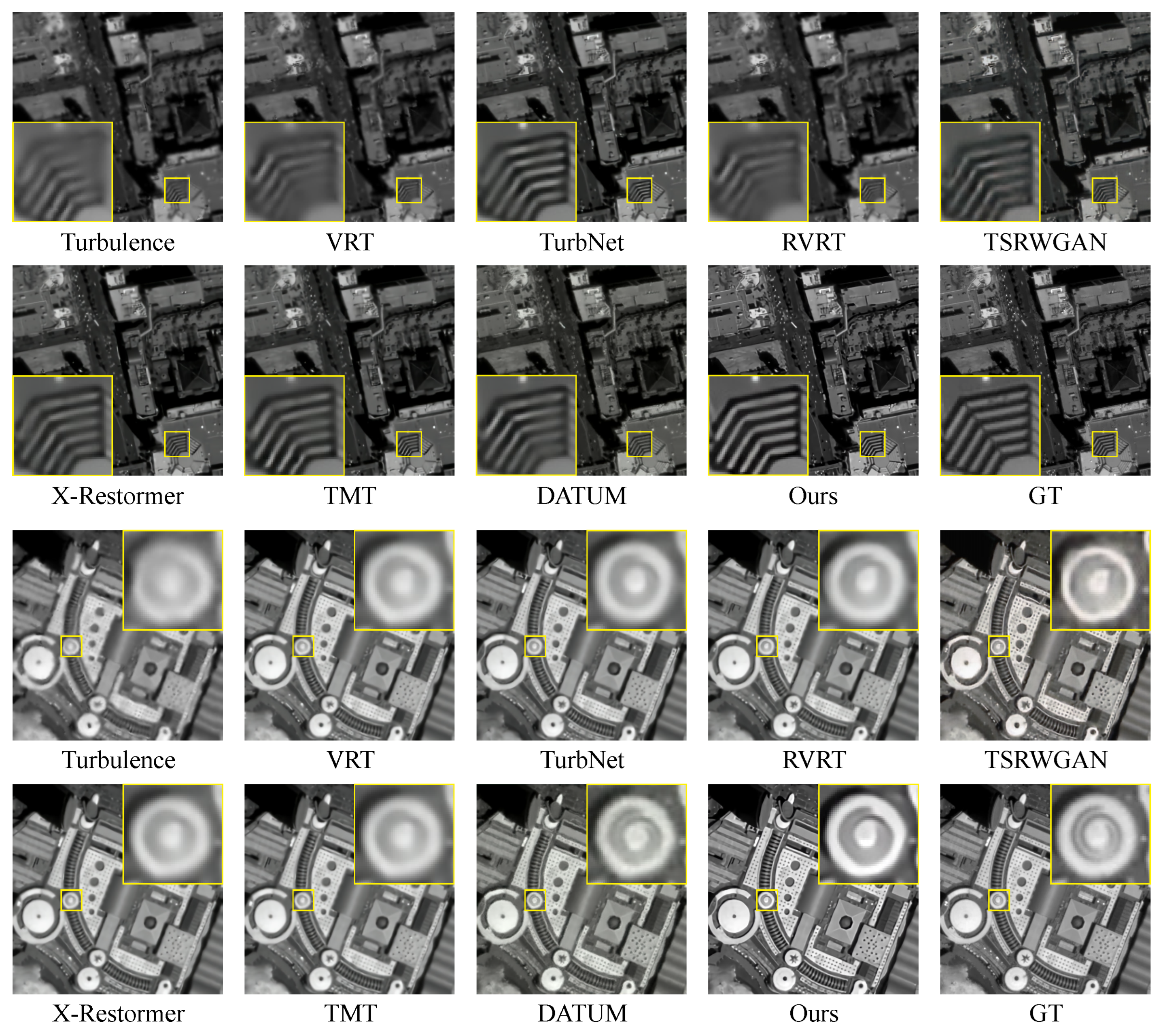
Figure 7.
Qualitative comparisons on scene-17 and scene-18 of Luojia3-01. Zoom in for better visualization.
Figure 7.
Qualitative comparisons on scene-17 and scene-18 of Luojia3-01. Zoom in for better visualization.
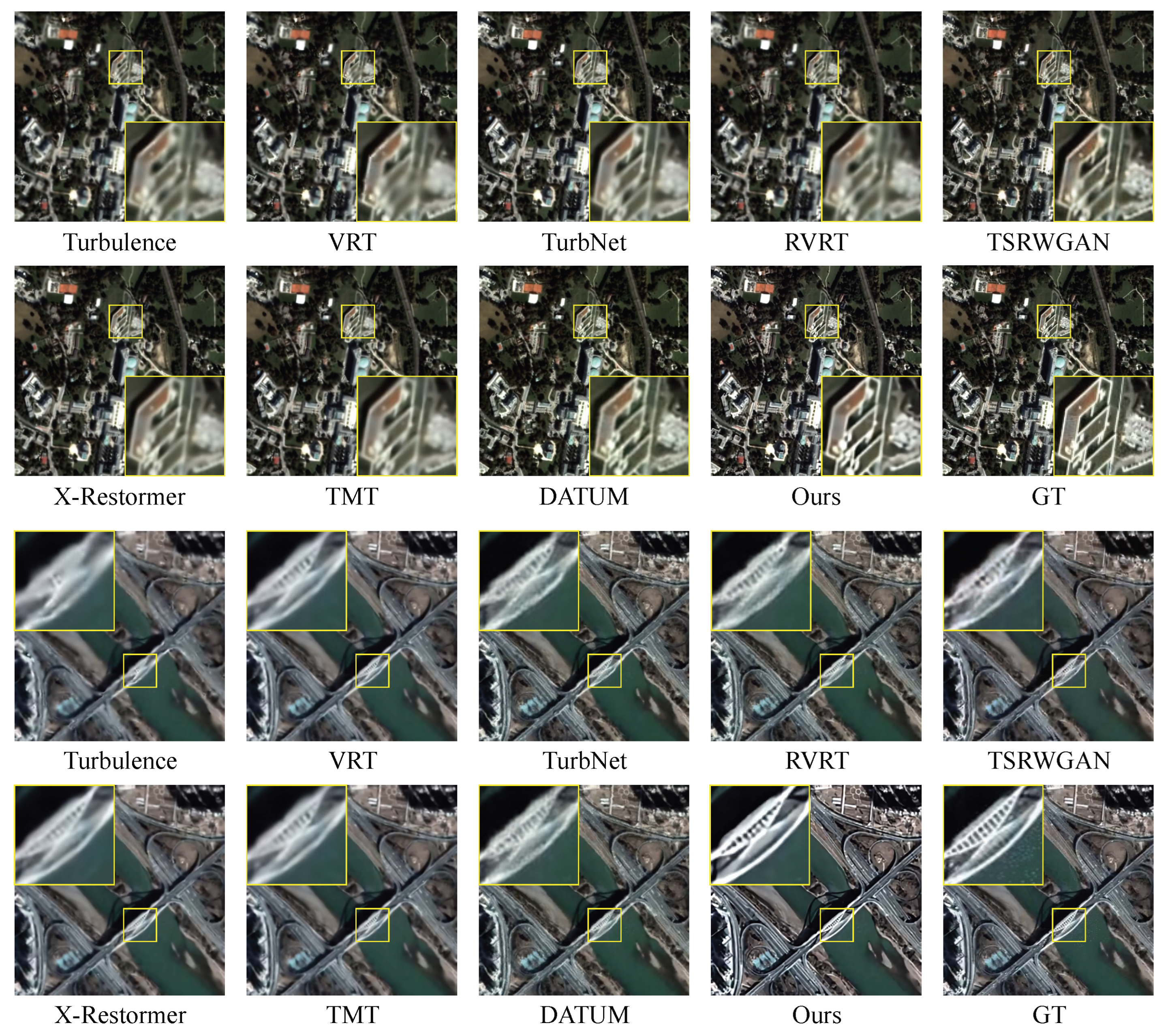
Figure 8.
Visualization comparison on real-world turbulence-degraded satellite videos. The original video sequences are sourced from the SatSOT dataset. Zoom in for better visualization.
Figure 8.
Visualization comparison on real-world turbulence-degraded satellite videos. The original video sequences are sourced from the SatSOT dataset. Zoom in for better visualization.
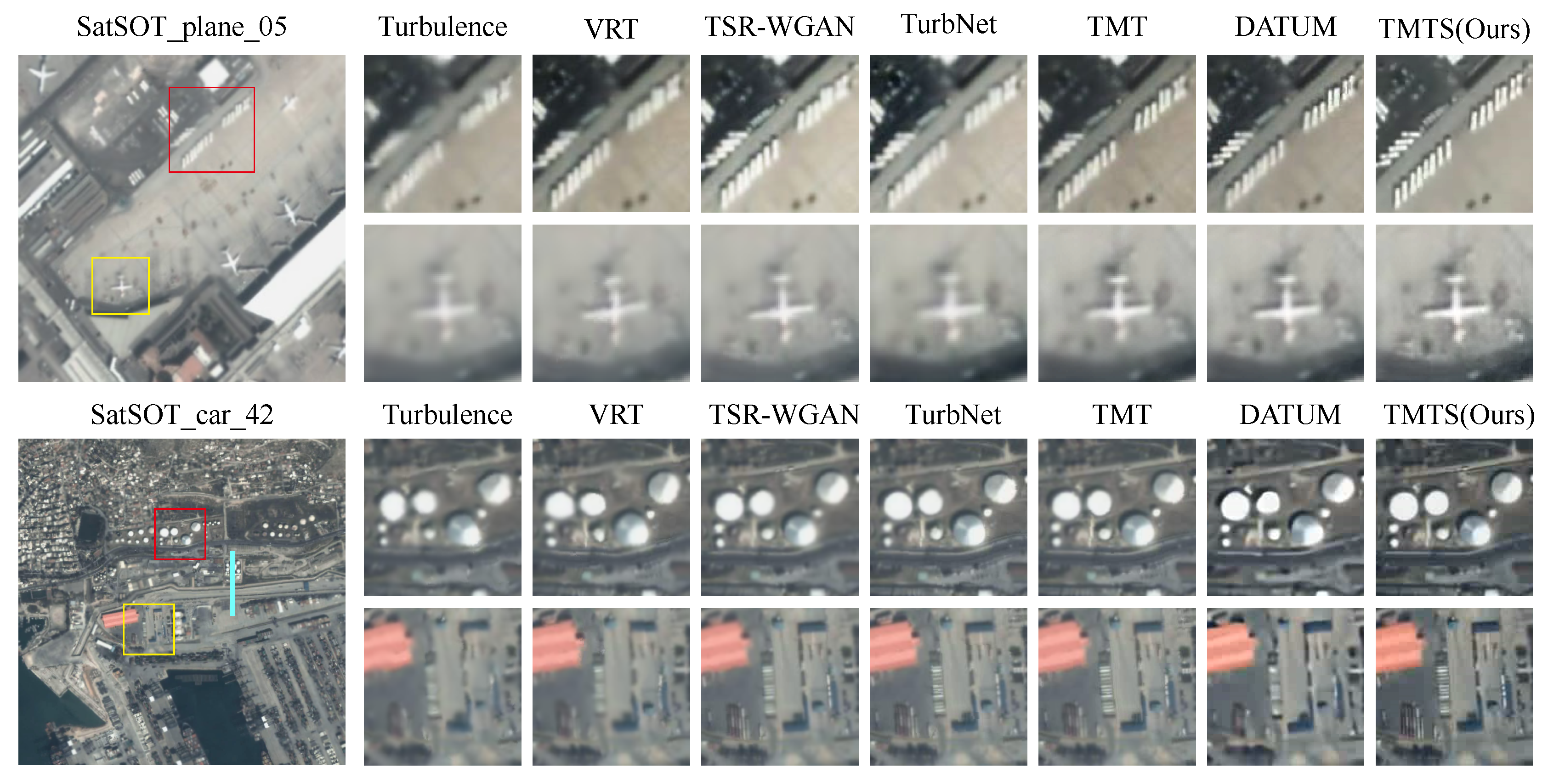
Figure 9.
Temporal-spatial (y-t) profiles of the "SatSOT_car_42" scene reconstructed via turbulence mitigation, generated by tracking an aqua-encoded pixel line across sequential frames with temporal stacking.
Figure 9.
Temporal-spatial (y-t) profiles of the "SatSOT_car_42" scene reconstructed via turbulence mitigation, generated by tracking an aqua-encoded pixel line across sequential frames with temporal stacking.
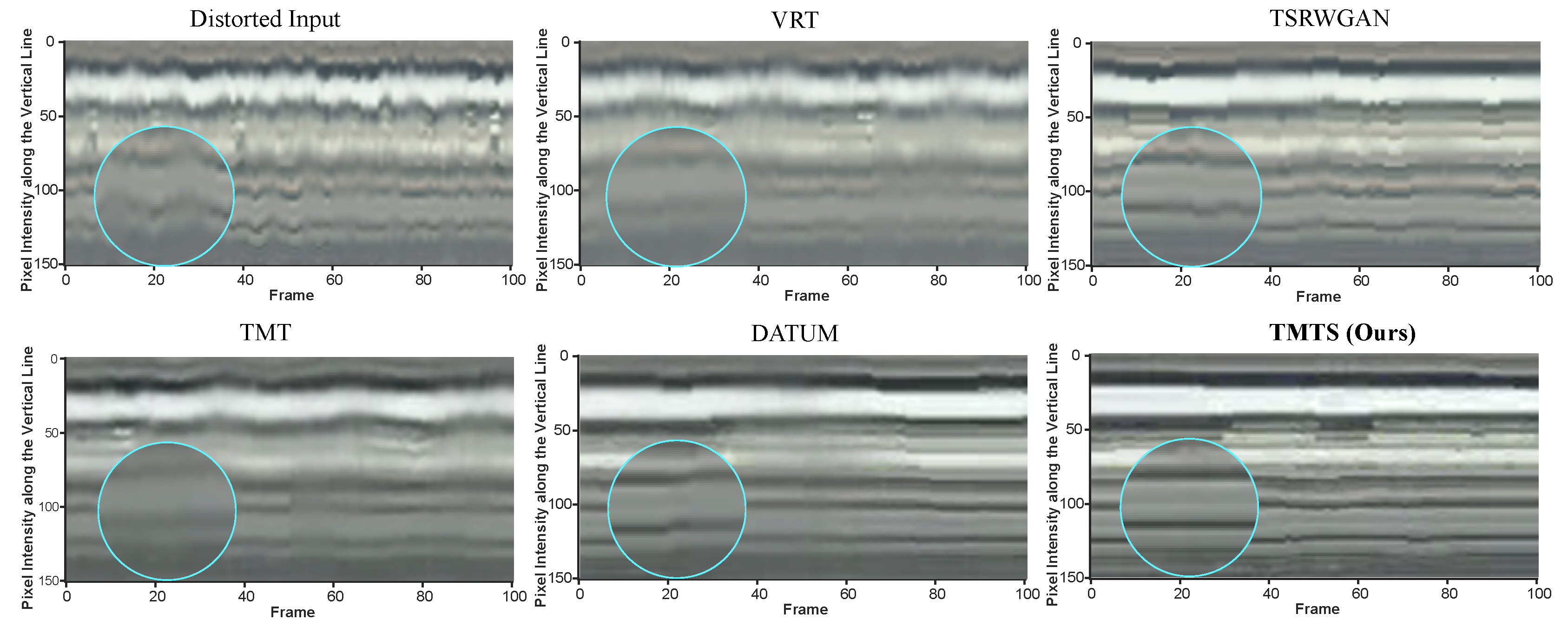
Figure 10.
Effectiveness of the turbulence signature modeling. (a) Turbulence-distored input. (b) Visualizations of the intermediate turbulence signature. (c) - (d) denote the repair effects without and with the turbulence signature, respectively.
Figure 10.
Effectiveness of the turbulence signature modeling. (a) Turbulence-distored input. (b) Visualizations of the intermediate turbulence signature. (c) - (d) denote the repair effects without and with the turbulence signature, respectively.
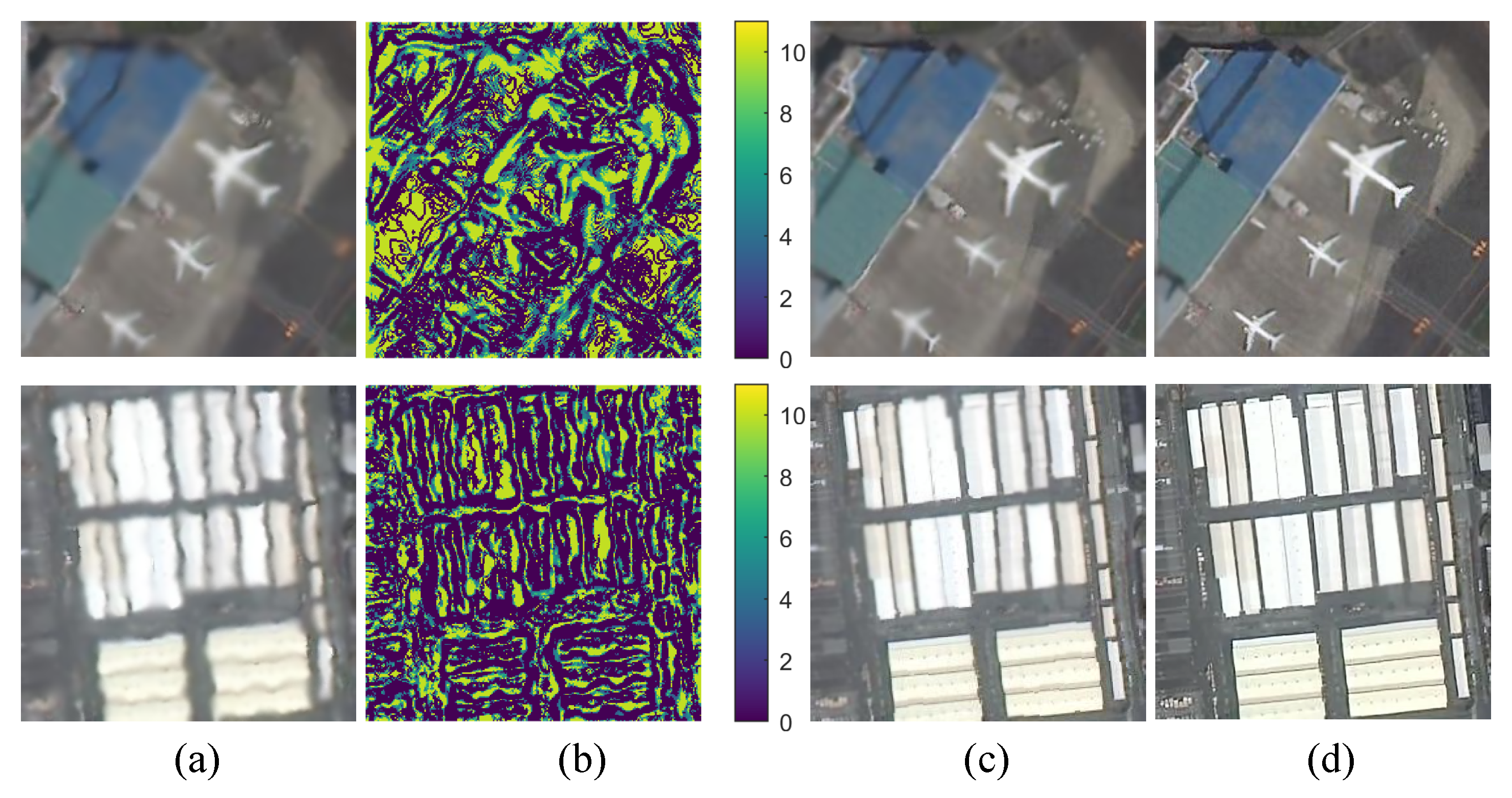
Figure 11.
Performance comparison of 10-, 20-, and 30-frame input models across multi-scale inference conditions.
Figure 11.
Performance comparison of 10-, 20-, and 30-frame input models across multi-scale inference conditions.
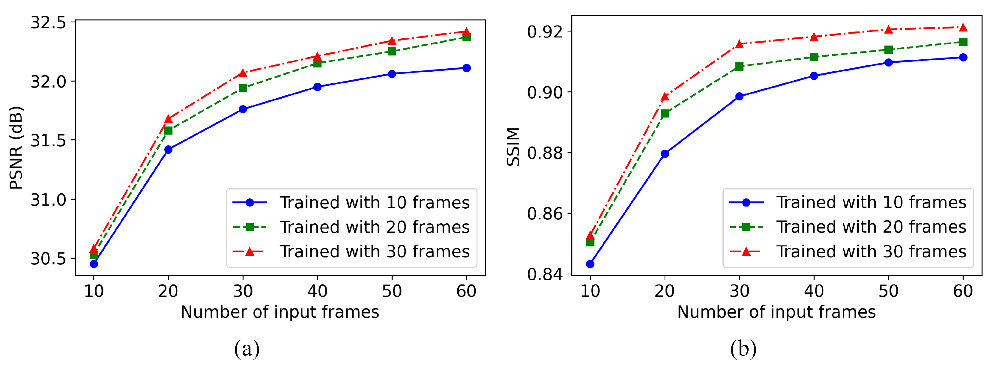
Figure 12.
Computational complexity-performance trade-off and real-time inference analysis: (a) FLOPs-Parameters-PSNR correlation in multi-scene evaluation; (b) Inference speed improvement over baseline architectures.
Figure 12.
Computational complexity-performance trade-off and real-time inference analysis: (a) FLOPs-Parameters-PSNR correlation in multi-scene evaluation; (b) Inference speed improvement over baseline architectures.
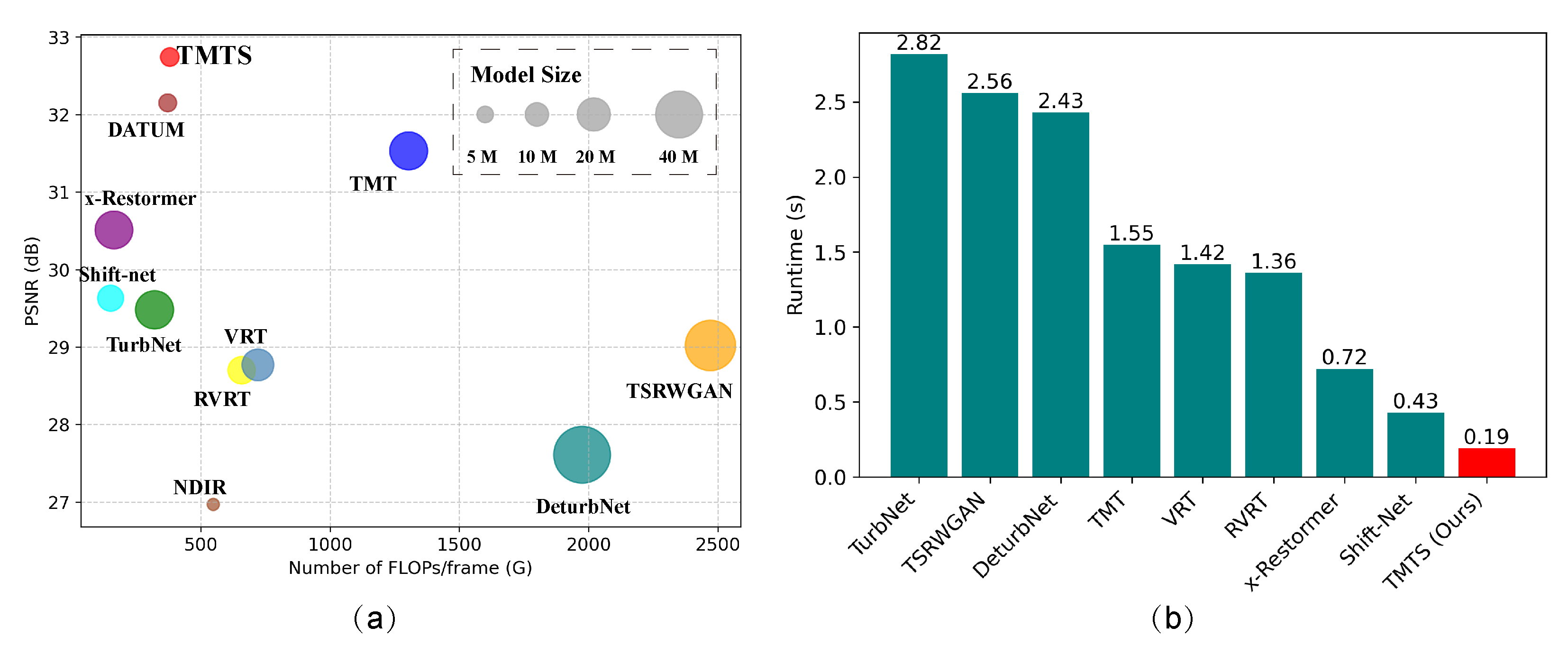

Table 1.
The properties of five video satellites involved in this paper, including Jilin-1, Loujia3-01, SkySat-1, UrtheCast, and Carbonite-2.
Table 1.
The properties of five video satellites involved in this paper, including Jilin-1, Loujia3-01, SkySat-1, UrtheCast, and Carbonite-2.
| Train/Test | Video Satellite | Region | Captured Date | Duration | FPS | Frame Size |
|---|---|---|---|---|---|---|
| Train | Jilin-1 | San Francisco | Apr. 24th, 2017 | 20 s | 25 | 3840 × 2160 |
| Valencia, Spain | May. 20th, 2017 | 30 s | 25 | 4096 × 2160 | ||
| Derna, Libya | May. 20th, 2017 | 30 s | 25 | 4096 × 2160 | ||
| Adana-02, Turkey | May. 20th, 2017 | 30 s | 25 | 4096 × 2160 | ||
| Tunisia | May. 20th, 2017 | 30 s | 25 | 4096 × 2160 | ||
| Minneapolis-01 | Jun. 2nd, 2017 | 30 s | 25 | 4096 × 2160 | ||
| Minneapolis-02 | Jun. 2nd, 2017 | 30 s | 25 | 4096 × 2160 | ||
| Muharag, Bahrain | Jun. 4th, 2017 | 30 s | 25 | 4096 × 2160 | ||
| Test | Jilin-1 | San Diego | May. 22nd, 2017 | 30 s | 25 | 4096 × 2160 |
| Adana-01, Turkey | May. 25th, 2017 | 30 s | 25 | 4096 × 2160 | ||
| Carbonite-2 | Buenos Aires | Apr. 16th, 2018 | 17 s | 10 | 2560 × 1440 | |
| Mumbai, India | Apr. 16th, 2018 | 59 s | 6 | 2560 ×1440 | ||
| Puerto Antofagasta | Apr. 16th, 2018 | 18 s | 10 | 2560× 1440 | ||
| UrtheCast | Boston, USA | - | 20 s | 30 | 1920 × 1080 | |
| Barcelona, Spain | - | 16 s | 30 | 1920 ×1080 | ||
| Skysat-1 | Las Vegas, USA | Mar. 25th, 2014 | 60 s | 30 | 1920 × 1080 | |
| Burj Khalifa, Dubai | Apr. 9th, 2014 | 30 s | 30 | 1920 × 1080 | ||
| Luojia3-01 | Geneva, Switzerland | Oct. 11th, 2023 | 27 s | 25 | 1920 ×1080 | |
| LanZhou, China | Feb. 23rd, 2023 | 15 s | 24 | 640 × 384 |
Table 2.
Quantitative comparisons on Jilin-T. The PSNR/SSIMs are calculated on the luminance channel (Y). The best and second performances are highlighted in red and blue, respectively.
Table 2.
Quantitative comparisons on Jilin-T. The PSNR/SSIMs are calculated on the luminance channel (Y). The best and second performances are highlighted in red and blue, respectively.
| Method | Scene-1 | Scene-2 | Scene-3 | Scene-4 | Scene-5 | Average |
|---|---|---|---|---|---|---|
| Turbulence | 24.96/0.7644 | 25.15/0.7743 | 22.97/0.7207 | 24.21/0.7670 | 24.35/0.7559 | 24.33/0.7564 |
| NDIR [35] | 25.45/0.8206 | 25.63/0.8308 | 24.33/0.7906 | 26.04/0.8262 | 25.12/0.8466 | 25.31/0.82296 |
| TSRWGAN [16] | 27.55/0.9122 | 28.75/0.9236 | 26.85/0.8918 | 26.63/0.8989 | 26.97/0.9071 | 27.35/0.9067 |
| RVRT [29] | 28.65/0.8817 | 26.44/0.8276 | 26.27/0.8762 | 27.33/0.8830 | 26.95/0.9044 | 27.13/0.8746 |
| TurbNet [14] | 27.03/0.8548 | 28.31/0.8663 | 25.28/0.8049 | 25.15/0.8263 | 26.35/0.8590 | 26.42/0.8423 |
| DeturbNet [15] | 25.61/0.8305 | 26.08/0.8327 | 24.27/0.7855 | 25.81/0.8409 | 25.74/0.8501 | 25.50/0.8280 |
| ShiftNet [36] | 29.31/0.9275 | 28.93/0.8757 | 27.62/0.8905 | 31.48/0.9357 | 30.34/0.9297 | 29.54/0.9118 |
| TMT [37] | 33.25/0.9331 | 32.67/0.9359 | 28.91/0.8989 | 33.27/0.9284 | 31.22/0.9267 | 31.11/0.9242 |
| VRT [38] | 28.49/0.8834 | 26.39/0.8232 | 26.30/0.8757 | 27.39/0.8875 | 26.92/0.9041 | 27.10/0.8748 |
| x-Restormer [39] | 30.16/0.8960 | 29.15/0.8601 | 28.54/0.8973 | 30.68/0.9034 | 30.27/0.9102 | 29.76/0.8934 |
| DATUM [18] | 33.15/0.9329 | 33.92/0.9517 | 29.66/0.9042 | 32.47/0.9571 | 31.97/0.9438 | 32.23/0.9379 |
| TMTS | 33.46/0.9461 | 34.17/0.9458 | 29.75/0.9046 | 32.53/0.9609 | 32.13/0.9390 | 32.41/0.9393 |
Table 3.
Quantitative comparisons on Carbonite-2 and UrtheCast. The best and second performances are highlighted in red and blue, respectively.
Table 3.
Quantitative comparisons on Carbonite-2 and UrtheCast. The best and second performances are highlighted in red and blue, respectively.
| Satellite | Method | Scene-6 | Scene-7 | Scene-8 | Scene-9 | Average |
|---|---|---|---|---|---|---|
| Carbonite-2 | Turbulence | 25.86 /0.7955 | 25.20 /0.7806 | 23.57/0.8161 | 22.85/0.7747 | 24.37/0.7917 |
| NDIR[35] | 26.42/0.823 | 27.56 /0.8090 | 26.97/0.8311 | 26.34/0.8309 | 26.82/0.8235 | |
| TSRWGAN[16] | 28.35/0.8649 | 29.04/0.8931 | 28.46 0.8742 | 27.11/0.8635 | 28.24 0.8739 | |
| RVRT[29] | 29.03/0.8833 | 29.70/0.9048 | 27.58 0.8859 | 28.82/0.8601 | 28.78/0.8835 | |
| TurbNet[14] | 30.56/0.9056 | 29.32/0.9285 | 27.37/0.9156 | 28.21/0.8738 | 28.87/0.9059 | |
| DeturNet[15] | 27.29/0.8696 | 28.14/0.8972 | 26.26/0.8714 | 27.43/0.8575 | 27.28/0.8739 | |
| Shift-Net[36] | 28.09/0.9098 | 28.52/0.8863 | 27.63/0.9141 | 27.82/0.8815 | 28.02/0.8979 | |
| TMT[37] | 31.48/0.9397 | 31.35/0.9220 | 29.62/0.9372 | 31.27/0.9029 | 30.93/0.9255 | |
| VRT[38] | 28.19/0.8991 | 28.77/0.8535 | 27.18/0.8674 | 29.51/0.8630 | 28.41/0.8708 | |
| X-Restormer[39] | 29.41/0.9135 | 29.36/0.9050 | 28.95/0.8983 | 30.55/0.8706 | 29.57/0.8969 | |
| DATUM[18] | 32.38/0.9405 | 32.23/0.9259 | 30.91/0.9316 | 31.68/ 0.9055 | 31.80/0.9259 | |
| TMTS | 32.69/0.9422 | 32.44/0.9328 | 30.75/ 0.9385 | 32.24/0.9018 | 32.03/0.9288 | |
| Satellite | Method | Scene-10 | Scene-11 | Scene-12 | Scene-13 | Average |
| Urthecast | Turbulence | 25.46 /0.8548 | 27.28/0.8610 | 24.56/0.8426 | 25.10/0.8415 | 25.60/0.8500 |
| NDIR[35] | 26.42/0.823 | 27.56 /0.8090 | 26.97/0.8311 | 26.34/0.8309 | 26.82/0.8235 | |
| TSRWGAN[16] | 29.69/0.9018 | 29.43/0.9293 | 28.18/0.9121 | 28.92/0.9079 | 29.06/0.9128 | |
| RVRT[29] | 29.04/0.8633 | 28.35/0.8915 | 27.62/0.8740 | 28.4/0.8963 | 28.35/0.8813 | |
| TurbNet[14] | 27.76/0.9005 | 28.72/0.8843 | 28.45/0.8764 | 27.34/0.8972 | 28.07/0.8896 | |
| DeturNet[15] | 27.29/0.8696 | 28.14/0.8972 | 26.26/0.8714 | 27.43/0.8575 | 27.28/0.8739 | |
| Shift-Net[36] | 28.27/0.9136 | 30.25/0.9305 | 31.24/0.9199 | 30.41/0.9268 | 30.04/0.9227 | |
| TMT[37] | 31.23/0.9267 | 30.36/0.9359 | 32.18/0.9424 | 30.64/0.9170 | 31.10/0.9305 | |
| VRT[38] | 29.96/0.9033 | 28.38/0.8966 | 28.53/0.9070 | 29.68/0.9052 | 29.14/0.9030 | |
| X-Restormer[39] | 31.42/0.9228 | 30.75/0.9312 | 31.66/0.9305 | 30.42/0.9103 | 31.06/0.9237 | |
| DATUM[18] | 32.56/0.9409 | 33.37/0.9452 | 32.16/0.9396 | 30.43/0.9355 | 32.13/0.9403 | |
| TMTS | 32.97/0.9368 | 33.82/0.9540 | 33.24/0.9437 | 31.05/0.9362 | 32.77/0.9427 |
Table 4.
Quantitative comparisons on SkySat-1 and Luojia3-01. The best and second performances are highlighted in red and blue, respectively.
Table 4.
Quantitative comparisons on SkySat-1 and Luojia3-01. The best and second performances are highlighted in red and blue, respectively.
| Satellite | Scene | TurbNet [14] | VRT [38] | TMT [37] | X-Restormer [39] | DATUM [18] | TMTS |
|---|---|---|---|---|---|---|---|
| SkySat-1 | Scene-14 | 31.10/0.9462 | 33.61/0.9493 | 30.49/0.9258 | 32.05/0.9296 | 33.86/0.9424 | 33.93/0.9430 |
| Scene-15 | 31.61/0.9299 | 33.08/0.9518 | 30.85/0.9145 | 32.33/0.9310 | 34.02/0.9558 | 33.86/0.9572 | |
| Scene-16 | 32.42/0.9233 | 32.52/0.9304 | 31.24/0.9167 | 30.68/0.9242 | 32.17/0.9575 | 32.77/0.9510 | |
| Luojia3-01 | Scene-17 | 33.18/0.9306 | 33.43/0.9418 | 30.06/0.9035 | 31.55/0.9304 | 33.21/0.9450 | 33.59/0.9453 |
| Scene-18 | 31.07/0.9273 | 32.31/0.9356 | 29.48/0.9085 | 31.60/0.9124 | 32.84/0.9389 | 33.29/0.9405 | |
| Average | 31.87/0.9315 | 32.99/0.9418 | 30.42/ 0.9138 | 33.39/0.9164 | 31.64/0.9255 | 33.49/0.9474 | |
Table 5.
Blind reference results on real-world satellite video. The best results are highlighted bold.
Table 5.
Blind reference results on real-world satellite video. The best results are highlighted bold.
| Method | VRT [38] | TurbNet [14] | TSRWGAN [16] | TMT [37] | DATUM [18] | TMTS(Ours) |
|---|---|---|---|---|---|---|
| BRISQUE (↓) | 48.8979 | 46.7041 | 46.2586 | 45.8577 | 44.0835 | 42.2954 |
| CEIQ (↑) | 2.9326 | 3.0831 | 3.1102 | 3.1793 | 3.3512 | 3.3458 |
| NIQE (↓) | 4.6137 | 4.4832 | 4.3419 | 4.1135 | 3.9943 | 3.8161 |
Table 6.
Ablation experiments on the effectiveness of each component.
| Components | Baseline (TSTSA) | + TSGA | + CGRFU | |||
| w/o TS | w TS | w/o TS | w TS | w/o TS | w TS | |
| PSNR (↑) | 30.15 | 30.41 | 31.67 | 32.05 | 32.52 | 32.74 |
| SSIM (↑) | 0.8765 | 0.8804 | 0.9113 | 0.9122 | 0.9206 | 0.9217 |
| #Param. (M) | 4.782 | 4.768 | 5.739 | 5.724 | 6.27 | 6.24 |
| FLOPs (G) | 306.5 | 304.2 | 352.8 | 349.7 | 381.4 | 377.6 |
Disclaimer/Publisher’s Note: The statements, opinions and data contained in all publications are solely those of the individual author(s) and contributor(s) and not of MDPI and/or the editor(s). MDPI and/or the editor(s) disclaim responsibility for any injury to people or property resulting from any ideas, methods, instructions or products referred to in the content. |
© 2025 by the authors. Licensee MDPI, Basel, Switzerland. This article is an open access article distributed under the terms and conditions of the Creative Commons Attribution (CC BY) license (http://creativecommons.org/licenses/by/4.0/).
Copyright: This open access article is published under a Creative Commons CC BY 4.0 license, which permit the free download, distribution, and reuse, provided that the author and preprint are cited in any reuse.


