

Submitted:
29 May 2025
Posted:
30 May 2025
You are already at the latest version
Abstract
The phenomenon of rising forward price volatility, both historical and implied, as maturity approaches, is referred to as the Samuelson} effect or maturity effect. Disregarding this effect leads to significant mispricing of early exercise options, extendible options, or other path-dependent options. The primary objective of the research is to identify a practical way to incorporate the Samuelson effect in the evaluation of commodity derivatives. We opt to represent the instantaneous variance and utilize the exponential decay parameterizations of the Samuelson effect. We develop efficient calibration techniques utilizing historical data from nearby futures and conduct analytics on statistical mistakes to establish a baseline for model performance. Utilizing 15 years of data for WTI, Brent, and NG, the study yields excellent results with the fitting error remaining well within the statistical error, except for the 2020 crisis period. We validate the stability of the fitted parameters by cross-validation approaches and assess the model's out-of-sample performance. The technique is applicable to seasonal commodities, including natural gas and electricity. We illustrate the application of the seasonal Samuelson model in extrapolating implied volatilities, which is crucial for the valuation and risk assessment of long-term contracts, such as widely utilized Power Purchase Agreements (PPAs).
Keywords:
volatility
; commodity
; term structure
; nearby futures
; seasonality
; exponential decay
1. Introduction
Understanding the dynamics of futures price volatility is very important for many aspects of risk management, such as hedging, portfolio construction, derivatives pricing and many other. Samuelson was the first who investigated the relation between volatility and time until contract expiration, stating the hypothesis that the volatility of futures price changes should increase as the delivery date nears. This prediction is very well known and referred to as Samuelson hypothesis, or maturity effect,1] This backwardation of volatility of forward contracts arises across most markets but this effect is especially pronounced in energy markets, as a particular steep increase in volatility occurs in the last six (or less) months of the life of the contract. This is one of the most fascinating phenomenon of commodity futures, which must be taken into account in pricing and managing of commodity contracts.
To illustrate the importance of this effect, we start with a simple example. We consider a future contract on WTI with expiration in years priced at per barrel. Assume that the implied volatility quoted for this contract is and we consider an ATM call option on this future expiring months before the contract expiration, thus in years. Such options are called early exercise options. The total variance during the lifetime of the contract will be . If we price the option using the quoted implied volatility, the price of the early exercise ATM call option will be per unit (no discount). However, under Samuelson effect the variance does not accumulate in uniform fashion, and such calculation will be wrong. Suppose we have a strong Samuelson, so that a half of the total variance happens in the last three months of the life of the contract. In such case, to price the option we have to use the volatility:
The right option price is , and ignoring the presence of Samuelson leads to overpricing the option by .
Now, let’s analyze the consequences of using a wrong variance for the second part of the time, the last three months of the lifetime of the contract. Since a half of the total variance realizes during a short period of time of three months, the average volatility corresponding to the last three months, will be much higher:
Assume that in years we have a right to buy a call option for premium , and the strike of the call option equal to the current forward price . Thus we consider a compound option with payoff:
where is the Black call price with price F of the underlying asset, strike , volatility and time to expiration . We can price the compound option by using standard numerical procedures ( grid evaluation or Monte Carlo). Even though the right with Samuelson is higher than with flat Samuelson, the expectation of the underlying call option is the same in two scenarios (we use a risk neutral pricing). However, the distribution of future prices in years with flat Samuelson is much wider ( standard deviation of future price of vs ), which makes the compound option more expensive under flat Samuelson vs with Samuelson . Disregarding Samuelson results in overpricing the option by .
Another examples of an early exercise options include swaptions, which are widespread products in Energy Markets. Their evaluation is discussed in [2]. Samuelson effect must be taken into account in evaluation of path dependent options, such as extendibles, calculations of forward exposure of a portfolio, necessary for CVA computations; hedging decisions and many other.
Numerous studies have investigated the Samuelson hypothesis empirically, and it has been supported in a subset of markets. Many of them arrive to mixed conclusions. For example, Miller [3] investigates live cattle, Barnhill et al. [4] study U. S. Treasury bonds; Adrangi et.al [5] consider selected energy; Adrangi and Chatrath [6] analyze coffee, sugar, and cocoa. Andersen [7] finds evidence in the agricultural markets, such as wheat, oats, soybean mean, cocoa, but not for silver. Milonas [8] finds strong support for the hypothesis in agricultural markets, but little or no support when using gold, copper, GNMA, T-bond, and T-bill prices. Rutledge (1976) finds support for the Samuelson hypothesis with silver and cocoa, but inconclusive evidence for wheat and soybean oil. Galloway and Kolb [10] study the term structure of volatility in 45 markets, including agricultural and energy commodity futures, precious and industrial metal futures, and stock index, currency, and interest rate futures. Their findings provide support for the maturity effect in agricultural and energy commodities, but not in precious metals and financials. Liu [11] employs almost stochastic dominance and the power spectrum to investigate the maturity effect for five groups of energy futures, such as crude oil, reformulated regular gasoline, RBOB regular gasoline, No. 2 heating oil, and propane. The outcome provides mixed results, ranging from supporting, to being contrary to the hypothesis. Jaeck and Lautier [12] find evidence of a Samuelson effect in various electricity markets, such as German, Nordic, Australian and US, and show that storage is not a necessary condition for such an effect to appear.
"Negative" papers rejecting the hypothesis include Grammatikos and Saunders [13] , who find no relation between futures return volatility and time-to-maturity for currency futures prices, and a study by Park and Sears [14] which provides evidence to disprove the Samuelson hypothesis for stock index. The well known study by Bessembinder et al. [15] suggests that the hypothesis will be generally supported in markets where spot price changes include a predictable temporary component, which likely to be met in real assets than for financial assets. They show that the hypothesis will generally be supported in markets where spot prices and convenience yields are positively correlated. The authors assume the carry arbitrage model represents futures markets.
The carry arbitrage model is based on the notion that the underlying instrument can be ‘‘carried” (purchased) with financing (borrowing) and delivered against a short futures position. Brooks [16] identifies and explores the important link between the empirical Samuelson hypothesis and theoretical carry: the degree to which carry arbitrage is empirically validated is associated with the degree to which the Samuelson hypothesis is not supported. In the continuation of the research, Brooks and Teterin [17] study the volatility term structure in 10 futures markets comprising three categories: agriculture, energy, and metals. To estimate the slope of the volatility term structure they use the Nelson and Siegel [18] functional form, borrowed from the literature on modeling the term structure of interest rates. The authors show that the slope of the volatility term structure is more negative when inventories are low and that the threshold for high/low inventory is specific to each market. The relationship between the Samuelson hypothesis and inventory levels is rooted in the cost-of-carry model
The popular models in the academic literature arrive to the Samuelson effect of futures volatility by considering models formulated in terms of the spot energy price with mean reverting process, see Clewlow and Strickland [19] The Schwatz single factor model, [20] results in the exponential decay of future volatility:
where is the mean reversion rate, and is the spot price volatility. The long term level of volatilities at is zero, which is not realistic. Two factors models with mean reverting processes for spot price and convenience yield, see Schwartz (1997), Gibson and Schwartz [21], Pilipović [22], result in an exponential decay of futures volatility with non-zero long term level volatility at long horizons.
The vital paper by Schwartz and Trolle [23] expands the framework of spot models to accommodate unspanned stochastic volatility. In their approach, the volatility of both spot price and forward cost of carry depend on two volatility factors which follow a mean reverting process, resulting in Samuelson effect for futures volatility. Crosby and Frau [24] broaden [23] model by incorporating multiple jump processes. They explore the valuation of plain vanilla options on futures prices when the spot price follows a log-normal process, the forward cost of carry curve and the volatility are stochastic variables, and the spot price and the forward cost of carry allow for time-dampening jumps. Frau and Fanelli [25] present a new term-structure model for commodity futures prices based on [23], which they extend by incorporating seasonal stochastic volatility represented with two different sinusoidal expressions and price plain vanilla options on the Henry Hub natural gas futures contracts. Hillard and Hillard [26] develop a jump-diffusion model for pricing and hedging with margined options on futures. They introduce a jump diffusion process for spot prices, and mean reverting processes for interest rate and stochastic convenience yield. Under positive correlations between diffusion parts futures volatility increases as maturity approaches. Model parameter are calibrated using data on Brent crude contracts.
Another class of models deal with modeling futures directly, not through spot prices and unobservable convenience yield. Chiarella et al. [27] propose a model encompassing hump-shaped, unspanned stochastic volatility, which entails a finite-dimensional affine model for the commodity futures curve and quasi-analytical prices for options on commodity futures. Schnieder and Tavin [28] introduce a futures-based model able of capturing the main features displayed by Crude Oil futures and options contracts, such as the Samuelson volatility effect and the volatility smile. They calculate the joint characteristic function of two futures contracts in the model in analytic form and use it to price calendar spread options.
Since the majority of trading in commodity happens in futures markets, we also choose to analyze futures directly. A natural generalization of the exponential decay model (1) (and appearing explicitly in various papers, (see for example [28]), is the following form of parameterization of variance with two exponential decays
where B is the global decay and is a long term decay (much smaller than B), is the normalization factor to match the implied market volatility, and is the level of a long term volatility. Swindle [29] uses this representation to model the total implied variance of commodity future.
We choose to model instantaneous variance using the representation (2). Introducing a time dependent instantaneous variance can be interpreted as non-uniform clock: we consider the total realized variance as "time". Under Samuelson, far away from the expiration the clock ticks very slowly, and it accelerates as we get closer to the expiry.
The Figure 1 below illustrates the point. In this example we use the simplest model (1) for instantaneous variance (thus ), and calculate the total variance (time) for a futures contract with expiry 5 years. Let the market implied volatility of the future be . We consider different choices of decay . Thus, from no Samuelson, to weak, moderate and very strong decay. In all cases the total realized variance between and the expiration T has to match the market implied variance , but the way it gets there depends on B. For a strong Samuelson , about of the total variance accumulates in the last year of the life of the contract.
In this paper, we devote our attention how to parameterize and more importantly, calibrate the increase of volatility when approaching contract maturity. We do not question the presence of Samuelson effect for considered commodity futures, neither we model the whole volatility surface, involving stochastic volatility models. Rather, we concentrate on Samuelson effect only and search for a practical solution which works, delivers stable results with error within the statistical model error. For that purpose, we employ the representation (2) for the instantaneous variance and consider two exponential decay models: a simpler model with long term decay , thus two parameters, called 1-decay model. Choice of modeling of instantaneous variance (or volatility) permits easy calibration to the market information ( implied volatilities) and calculation of variances on any future time intervals, using the aforementioned non-uniform clock.
We opt for using data of nearby contracts and normalize the variances of their returns by the variance of the prompt contact. We develop analytics for statistical errors on normalized variances using results by Joarder [30] to attain a benchmark for the calibration results, and present out of sample testing of the model. In our study we used 15 years of history for WTI, Brent and Natural Gas futures prices, 2006 - 2021, including the drama of Spring 2020. We generalize the calibration methodology to seasonal commodities such as natural gas. We contrast Samuelson strength vs the models performance in different historical periods. At crisis times, when Samuelson is strong, one should use 2-decay model, as it gives better results. From the other hand, at quiet times, therefore weak Samuelson, 1-decay model is totally adequate.
The closest research to our paper in the existing literature is the mentioned paper by Brooks and Teterin ("BT") [17]. They also use nearby future returns, calculate the their standard deviations and fit a three factor parametrization by Nelson and Siegel [18] with exponential decay. However there are key differences between our approaches. First, BT interpolate futures prices with Nelson-Sielge curve [18], resulting is a vector of futures pseudo-price time-series with each time-series corresponding to an exact maturity on every trading day. 1. We use the raw prices of nearby future contracts, not mixing them. Even though as calendar time passes, the time to expiration of nearby future indeed changes and drifts to zero, 2 we deliver convincing results of the volatility–maturity relationship using raw prices.
Second, BT employ only 12 nearby contracts, while we include all available information, 60 contracts. BT do not account for seasonality when considering term structure of NG volatility. Our data includes crisis period of Spring 2020, which is quite interesting period to test models.
Third, the models and the target of the fit are different. The NS model [18] model for yield curve given by the parametric form
is based on the forward yield curve, see Diebold and Li (2006):
BT use (3) to model average volatility of a synthetic forward contract with constant maturity (in months). We fit instantaneous variance employing a representation (2) similar to (4), but with two exponential decays. For us, the main input in the model, governing the Samuelson strength, is given by exponential decay parameter B. In the BT’s approach, the exponential decay parameter is fixed at the initial stages of the fit, and the main parameter reflecting the Samuelson forte, is represented by the slope of the volatility term structure .
Lastly, and most importantly, our main motivation is to find a natural and practical method to accommodate Samuelson effect in the evaluation of path dependent options, early expirations options, CVA, etc. That is why we choose the instantaneous variance as a subject of our study. This choice allows us to match the market information such options quotes on futures perfectly (through implied volatilities). BT [17] aim to test the Samuelson hypothesis for variety of commodities and link the Samuelson strength to inventory levels and carry arbitrage.
We generalized the calibration methodology to seasonal commodities such as Natural Gas. The Natural Gas term structure is defined by seasonality. Natural gas storage is a vital part of the natural gas delivery system and helps to balance supply and demand. During the winter season, from November to March (withdrawal season), gas consumption peaks as a result of increased heating demand. During the summer season, from April to October (injection season), gas demand decreases while production continues. Because of this, we fitted Samuelson independently after dividing the data for nearby futures into two periods: winter and summer. Since we used data of nearby contracts, with this separation, we were not allowed to concatenate returns from different seasons, for example, March and April. For that reason, we were forced to use only two months data of observation period. Despite the good fitting results, where the errors stayed largely within the statistical error, the results are not consistently stable due to the short observation period. Adding more seasons would cause even greater issues.
Next target was to find the methodology for Samuelson effect for a more complicated case of seasonal commodities, in particular electricity futures. Electricity always has been the most fascinating commodity to study due to non-storability (at least in meaningful quantities), therefore very high volatility and abundance of extreme events. Because supply and demand have to be in equilibrium at all times, the electricity seasonality is more refined that any other seasonal commodity. Each hour in each weekday and month has its own pattern and can be traded separately. Therefore, using only two seasons would not be enough, and we need to come up with a more granular seasonal model. The previous seasonal model for Natural Gas implies that is roughly the same for months in the same season, and the Samuelson parameters B, and are different for winter and summer months. Since we used only two months of nearby futures data, we were catching the Samuelson effect locally, at that particular period of time. The goal is to come up with a methodology which applicable to long term deals, such as popular Power Purchase Agreements ("PPA"), which become increasingly more popular in view of growing use of renewable energy. We use the same model for the instantaneous variance (2), with , however there is a number of differences between two approaches. Firstly, we assume that the normalization constant depends on a month in year, and the Samuelson parameters B and are the same for all months. We consider only the 1-decay model with . Secondly, we use the real futures data and calculate the realized variance on one year observation period. As in the previous model we calculate the ratios of variances, but now we use the variances of the same calendar month. We average the ratios for 12 moving the observation period and fit the model. The results are stable.
We demonstrated how the Samuelson effect can be used for commodities derivatives. Firstly, we outline the evaluation of early expiration options, such as swaptions. Secondly, we demonstrate how the calibrated model of the instantaneous variance can be used to extrapolate implied volatilities, which is crucially important in the evaluation of PPA’s. Furthermore, we discovered an intriguing application of the Samuelson effect to a popular auto-callable equity derivative, the snowball, see [31]. The term ”snowball” describes an investor’s potential for profit accumulation. Snowball is type of auto-callable structure with two barriers: knock-out and knock-in set up as percentage of the initial price.The longer the investor retains an income certificate, the more is the profit, provided the underlying does not drop precipitously. Consequently, the payment of the snowball is contingent upon the realized variance of the underlying asset and the rate of its accumulation. Issuing auto-callable derivatives on assets influenced by the Samuelson effect can be beneficial, as initial low volatility may extend the duration of the asset remaining within barriers, hence yielding greater profit. Furthermore, we identified that, based on the structure of a snowball, keeping the realized variance constant, there is an optimal rate of variance growth that yield maximum profit.
We now outline the remainder of the paper. Section 2 describes various calibration procedures, including generalization for seasonal commodities as Natural Gas. Section 3 discusses the results of the calibration using 15 years of data for Wti, Brent and Natural Gas futures, the optimal choice of observation period and the model selection, the analytics of the statistical errors to access the goodness of the fit. Section 4 outlines the calibration procedure of the Samuelson effect for electricity futures and presents the results using the historical data of North Hub Ercot electricity futures. Section 4 concludes. Some of the details are given in Appendix.
2. Calibration Procedures of Samuelson
This section is devoted to the detailed description of the calibration of the Samuelson effect.
To investigate the Samuelson effect, we begin with a selection of data. A variety of data types can be used to calibrate a certain Samuelson form. We can start by using a snapshot of the implied at-the-money volatility of the market. Analyzing the historical realized volatilities of returns of futures contracts with expirations , calculated a time period , , is a further choice. Lastly, the third option would be to examine the return volatilities of nearby contracts. We can use the idea of "promptness" of a contract in place of specific contracts. The first nearby contract, also known as the prompt, is the closest future contract that is accessible at time t and has the shortest duration to expiration. The second nearby contract is the next accessible contract, etc. The second neighboring contract takes over as the first one when the first one expires, etc. We can define an i-th nearby contract in general.
With the Samuelson effect, we anticipate lower volatility for farther-off futures. Utilizing data sources such as market indicated volatilities and forward-looking information has benefits. Option liquidity on futures longer than a year is, nevertheless, insufficient. There have been previous occasions when we have not observed an immediate decrease in volatility, which may be due to local market disturbances. However, historical realized volatilities reveal that realized volatilities almost usually decrease with expiration . Below is a picture of the WTI futures implied volatilities from December 2018 up to November 2019.
Since our approach is based on modeling instantaneous variance, the second source of data would involve integration to arrive to realized variance. Therefore, we choose to employ nearby contracts to capture the "true" instantaneous volatility. Thus, approach 3—the volatilities of returns of nearby contracts—is the data of choice for our analysis.
In order to eliminate the impact of volatility level and make the statistics comparable, we normalize the variances of the i-th nearby contract by the variance of the first nearby contract:
These ratios provide the basis of the calibrating processes. In Joarder (2009), the statistical characteristics of the product and ratio of two correlated chi-square random variables were investigated. The paper’s findings will be used to calculate the statistical errors of the ratios. The Appendix C will contain the specifics.
We establish a set of model parameter :
and model ratios that are inferred from the instantaneous variance’s form (2):
where where and are times to maturity (in years) of the i-th and the first nearby contracts correspondingly.
The general model calibration process adheres to the accepted methodology for determining which model parameters best fit the historical data. First, we choose an observation period and construct series of nearby contracts of historical settlement prices observed daily at and , , . For non-seasonal commodities, we used observation periods of two and twelve months, while for seasonal goods, we used two months. A two-month observation period usually equals M = 44, and a twelve-month observation period equals M = 252. N is the number of observed contracts, usually N = 60, and . After that, we compute log-returns.
We next compute realized variances of returns and document the previously established ratios. A constrained minimization of the total error determines the optimal set of model parameters
where are the model ratios given by (6). We assume that decay occurs mostly due to increase in and cancel out the normalization constant . The specific choices parameters and the constraints are revealed in each case.
The primary challenge of the minimization problem is the possibility of various solutions because of the way parameters influence the ratios: an increase in long-term volatility weakens the decay, whereas a higher B drives ratios to decay more quickly. We should stay away from certain areas of the parameter space where slight adjustments to ratios result in significant changes to decay or long-term volatility. Several contour plots of the 12-month ratio for the scenario where the long-term decay . are shown in the following Figure 3 to demonstrate this.
The model with two decays, B and , will be referred to as the 2-Decay model, whereas the model with will be called the 1-Decay model. Only in times of crisis, when Samuelson is very strong, do we need to use a more intricate 2 Decay model. The following section will provide examples.
2.1. Samuelson Effect for Seasonal Commodities
To accommodate Samuelson, the previous approach must be modified for seasonal commodities such as electricity, natural gas, heating oil, and gasoline. Our first emphasis is on natural gas, one of the most significant and "physical" commodities. The first seasonal model for Natural Gas assumes that is roughly the same throughout months within the same season, and the Samuelson parameters B, and are different for winter and summer months.
The subsequent objective was to identify the methodology for the Samuelson effect in a more complex scenario involving seasonal commodities, specifically electricity futures. Seasonality is more nuanced for electricity than for any other seasonal commodity. Every hour of each weekday and month exhibits a distinct pattern and can be traded independently. Consequently, relying solely on two seasons is insufficient; we must develop a more detailed seasonal model. We employ the identical model for the instantaneous variance (2) with while positing that the normalization constant is contingent upon the month of the year, while the Samuelson parameters B and remain constant across all months. We utilize actual futures data to compute the realized variance over a one-year observation period. Similar to the prior model, we compute the ratios of variances; however, we now utilize the variances from the same calendar month. We compute the average ratios over a 12-month period, adjusting the observation timeframe, and subsequently fit the model. The results are stable.
2.1.1. Natural Gas
A typical monthly supply-demand chart for natural gas (NG) based on EIA data is shown in the Figure 4. This type of chart can be found in many natural gas market references, such as Swindle (2014). Particularly during the winter, storage is essential to closing the gap between supply and demand.
There are significant winter peaks in demand because of the cold weather, and milder summer peaks because of rising power use. Demand is cyclical, which causes seasonal patterns in prices and volatility. This makes a volatility term structure a superposition of decay with time to expiration and seasonal shape. An illustration of implied NG natural gas volatility can be found in Figure 5.
Based on the data and the widely accepted description of natural gas storage seasons, we also choose to divide the Samuelson data into two periods: a summer (injection) season that runs from April to October, and a winter (withdrawal) season that runs from November to March.
Because of this division, we are unable to combine returns from various seasons, such March and April. Using an observation period of just one month is an easy fix. Fitting results are not convincing, though, because variance measured on (about) 22 data points is extremely noisy. As a result, we chose a two-month observation period, but we choose it carefully. For example, in September and October we observe first nearby futures prices from different seasons, therefore this period does not work. There are even more issues if we use additional months in the observation period, such as four or six, because we would have to leave out more combinations. Therefore, we decide to employ two months for the study time.
Using a similar process to that used for oil, mutatis mutandis, we fit a seasonal Samuelson independently.
2.1.2. Electricity
Electricity has consistently been the most intriguing commodity to examine due to its non-storability (at least currently, in significant quantities), resulting in considerable volatility and a prevalence of extreme events. Due to the necessity for supply and demand to be in equilibrium at all times, electricity seasonality is more nuanced than any other seasonal commodity, seen in both prices and volatilities.
Given this behavior, we formulate the subsequent assumptions regarding the dynamics of instantaneous variance (2).
- We presume .
- The parameters B and remain constant throughout the year.
- The normalization constant solely dependent on the month of the year and remains constant throughout all years.
We will now proceed to outline the methodology for calibrating the Samuelson parameters B and by utilizing historical data of prospective prices that have been observed over a one-year period. Assume that the year 2022 is the desired observation period. We select the initial contract as the contract that we observed until its expiration during the observation period, which in this case is January 2023.
We adhere to the subsequent steps:
- Record prices for the chosen contract for about one year prior to the expiration. In this particular instance, observations commence at time , January 1, 2022, and continue until the contract’s expiration at , contingent upon the market. 3 The observation period is defined as .
- Calculate log-returns and their standard deviation . This represents the realized volatility of the first contract.
- Simultaneously compute the log-returns of further forward contracts, including Feb 23, Apr 23, and extending four years forward to Dec 27, with the identical observation period , and determine the standard deviations of their log-returns. Document 48 realized volatilities
- Calculate ratios by dividing the volatility of each month and year by the volatility of the same month in the previous year:
- Record 36 ratios which are functions of and only on the presumption on the assumption on the normalization constant .
Subsequently, replicate the aforementioned steps 1-4, commencing on February 23, while advancing the observation term by one month, initiating from February 1, 2022, until the contract’s expiration. The approach yields an additional set of 36 ratios. Select March 23 and continue until December 2023. Consequently, we shall obtain 12 sets of 36 ratios. Observe that the time periods and are approximately same across all sets.
Given that they rely solely on times rather than the month of the year, we can average each promptness i across 12 sets to determine the optimal parameters B and that encapsulate the Samuelson effect.
Our objective is to develop a methodology suited to long-term agreements, such as prevalent Power Purchase Agreements (PPAs). Consequently, we have opted to examine a global pattern of volatility term structure, rather than a more detailed seasonal decay as conducted in our analysis of natural gas.
We will now describe the outcomes of the calibration tasks.
3. Results
This section examines the calibration results using 15 years of data for WTI, Brent, and Natural Gas futures, along with the selection of the observation period and the model (1-Decay versus 2-Decay). A 12-month observation period for WTI and Brent, a 2-month duration for natural gas, and a first-order decay model tend to be efficacious. During crises, when the Samuelson effect is significant, it is essential to employ a more refined 2-Decay model. We provide analytics for statistical errors on normalized variances to provide a baseline for calibration results and assess the error relative to the lower bound of the statistical error for WTI and Brent. To achieve this, we utilize a rolling window of 12 months (183-day interval). We conclude that, for a majority of times, excluding the crisis years of 2009 and 2020, the model aligns effectively with the data within the bounds of statistical error.
We also show the calibration results of the Samuelson effect for electricity futures at significant trading hubs, including Ercot North in Texas.
We commence with an examination of the descriptive statistics of the log returns for WTI, Brent, and Natural Gas futures.
We start with review of the descriptive statistics of log returns of WTI, Brent and Natural Gas futures.
3.1. Descriptive Statistics
We meticulously examine the returns of the initial four proximate contracts. We label the first nearby contract series of WTI as WTI1, the second nearby as WTI2, and so forth. Correspondingly, we assign the names of the contracts Brent1 to Brent4 for Brent Oil futures and NG1 to NG4 for Natural Gas. The findings are displayed in Table 1. The standard deviations are daily and increase as maturity approaches. We opt to exclude the negative price date for WTI contracts to prevent complications in the calculation of log returns.
3.2. Results of Samuelson Calibration, WTI, Brent and Natural Gas
We conducted the fitting technique multiple times throughout a designated observation period for WTI, Brent Oil, and Natural Gas. Table 2 enumerates the outcomes of WTI calibration throughout a 12-month observation period. The last column denotes the root mean square error (8) computed using the optimal parameters of the 1-Decay model, scaled by the volatility of the prompt contract.
For a typical example, we examine the instantaneous volatility of WTI realized during a 12-month observation period, from to , with . Figure 6 illustrates a fitting graph. The scatter dots denote the actual realized volatilities, whereas the line graphs illustrate the fitted model with exponential 1-decay. We calibrated the volatility level by aligning with the volatility of the immediate contract.
The Table 3 presents details on the RMSE errors for Brent over several observation periods.
To examine a seasonal instance of NG, we classify the data into two categories: summer, including April to October, and winter, spanning November to March. We eliminate inter-seasonal combinations and thereafter adjust the parameters for each season accordingly. Due to seasonality, we can only employ two months of return data. As a result, the assessments of true instantaneous volatility demonstrate increased noise. The model may not correspond as accurately as it does with WTI, however it sufficiently represents seasonal fluctuations. The subsequent table presents the calibration results for NG across various time periods.
3.3. Results of Samuelson Calibration for Electricity Futures
3.3.1. Ercot Markets
We begin with the Ercot (Electric Reliability Council of Texas) market, which is very unique and is widely known for its significant price volatility. It is an energy-only market, which means generators are only compensated for the energy they give to the grid, unlike other markets that also compensate for capacity availability. ERCOT added another component to wholesale prices in 2015, a scarcity adder. This scarcity adder represents the value of additional resources to grid reliability Further, ERCOT’s electricity system operates within Texas and is not subject to federal control by the Federal Energy Regulatory Commission (FERC). ERCOT’s transmission grid is solely contained inside the state of Texas and is not linked to other states’ networks. These two facts make ERCOT an "energy island".
ERCOT’s electricity prices are volatile due to several factors, including Texas’s unique weather patterns, its independent electrical grid, increasing demand, and the integration of intermittent renewable energy sources such as wind and solar. In February 2021, extremely low temperatures during Winter Storm Uri forced significant generation equipment to freeze, leading to prolonged outages throughout most of Texas. The scarcity adder resulted in elevated ERCOT energy prices, which remained at the price ceiling of /MWh for three consecutive days.
Due to the inherent volatility of electricity contracts, we cannot anticipate flawless fitting results as seen with WTI. The objective is to capture the general decline in volatility by calculating average seasonal ratios as outlined in section 2.1.2. The liquidity of energy futures tends to concentrate within the initial two to three years. Consequently, we employed only 24 ratios to calibrate Samuelson.
The graph below depicts the realized seasonal ratios in comparison to model ratios determined as of January 2021. This indicates that we computed the average of seasonal ratios for future contracts from January 2020 to December 2020. The fitted Samuelson is strong, which is unsurprising given that the period encompasses the Covid era.
Figure 8.
Calculated Seasonal ratios vs model ratios, ,
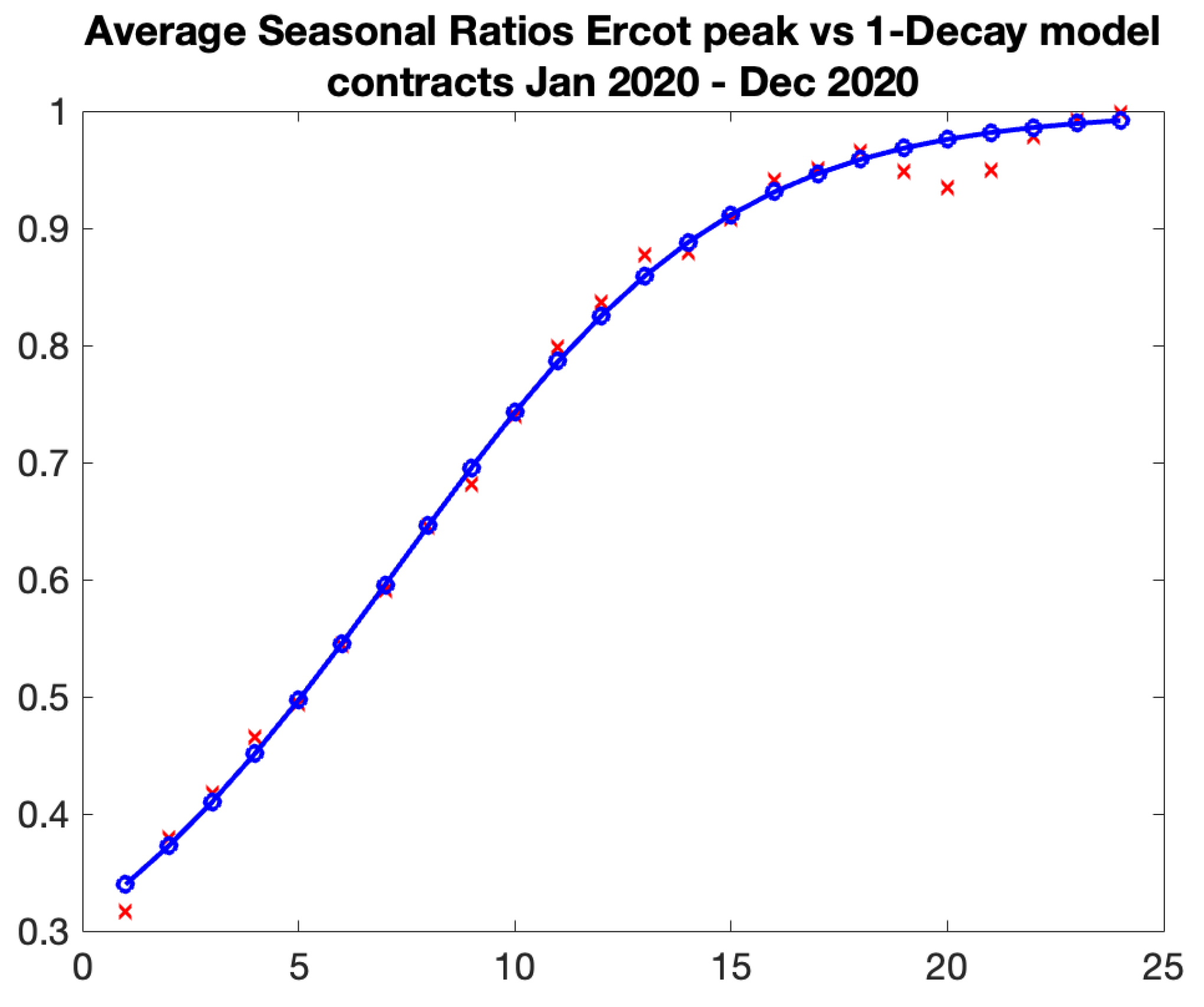
The aforementioned result is the best. Not all ratios fit as well, but we can usually identify the trend. The following is a more recent result of fitting the average of realized seasonal ratios from June 23 to May 24.
Figure 9.
Calculated Seasonal ratios vs model ratios, ,
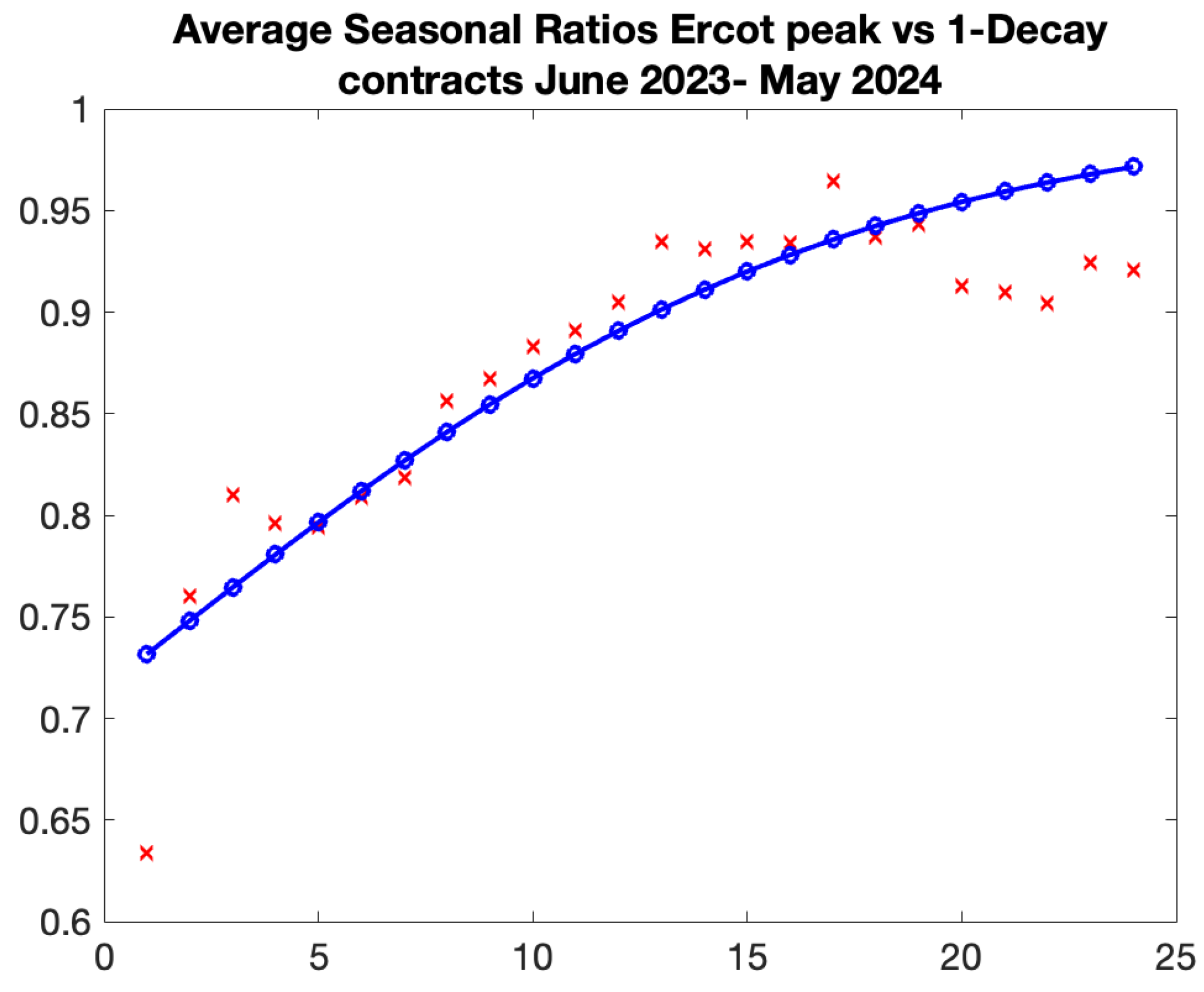
The following table shows the results of the Samuelson effect calibration for Ercot electricity futures. We record the parameters at the start of each year, using an average of 12 seasonal ratios from January to December of the preceding year.

Table 5.
Calibrated Samuelson Parameters, Ercot electricity futures.
| As of | B | |
|---|---|---|
| 1/1/18 | ||
| 1/1/19 | ||
| 1/1/20 | ||
| 1/1/21 | ||
| 1/1/22 | ||
| 1/1/23 | ||
| 1/1/24 |
3.4. Finding the Optimal Length of Observation Period
The length of the observation period is essential for volatility computation and calibration processes. We offer the subsequent considerations for selecting the length.
Calculating instantaneous volatility with one-month data from nearby contracts is suboptimal, as 22 data points may yield a noisy outcome. The confidence interval for the volatility estimate would be significantly wide. Consequently, we opted for a minimum observation time of two months. A two-month observation period may be a sensible choice, particularly during crisis times. For instance, in the spring of 2020, global market volatility was exceedingly high, and conditions were rapidly evolving. Utilizing two months may be a judicious decision. In a less volatile market, such as in 2019, one may opt for 6-month or 12-month periods to stabilize the calibrated parameters. A 12-month observation period is optimal, as it consistently encompasses the most liquid December contract. Another argument supporting the utilization of a 12-month observation period is the stability of fitted parameters when employing 12-month rolling data.
In conclusion, the selection of a 12 month observation period is our preference and primary case study.
3.5. Model Selection
Upon analyzing the results of the fit across several historical periods, we conclude that the 1-decay model yields fair results in comparison to the 2-decay model in the majority of periods. During stable market conditions, devoid of significant disruptions like the Covid-19 crisis in 2020 or the 2009 financial crisis, it is entirely justifiable to utilize the parsimonious 1-decay model.
Figure 10 illustrates a comparison between the 1-Decay Exponential model and the 2-Decay Exponential model. The black line illustrates the graph of the fitted 1-Decay Exponential model, while the blue line depicts the graph of the 2-Decay Exponential model. The observed realized volatilities in the tail exhibit a clear decay of long-term volatility. The 2-Decay Exponential model more accurately reflects the pattern, resulting in an improvement of around 80 basis points in RMSE accuracy. In 2009 and 2020, the 2-Decay model has far better performance. Similar patterns emerge during periods of market volatility, namely during the crises of 2009 and 2020.
Table 6.
WTI Calibration Results: 1 Exponential Decay Model vs 2 Exponential Decay Model, "1-D" denotes 1-Decay model, whereas "2-D" stands for 2-Decay model.
Table 6.
WTI Calibration Results: 1 Exponential Decay Model vs 2 Exponential Decay Model, "1-D" denotes 1-Decay model, whereas "2-D" stands for 2-Decay model.
| B | b | RMSE | ||||
|---|---|---|---|---|---|---|
| 2-D | ||||||
| 1-D | 0 |
3.6. Statistical Errors on the Normalized Ratios
To evaluate model performance, we developed analytics on the statistical errors of the normalized ratios as defined by (5). We begin with log-returns (7) of nearby contracts, which have a multivariate normal distribution. The ratio of the variance of the i-nearby contract, normalized by the "true" variance , follows a chi-square distribution with m degrees of freedom, where and M equals the number of observations.
Define and . The joint distribution of and is referred to as the bivariate chi-square distribution. Joarder (2009) examined the distribution of the product and the ratio of two correlated chi-square random variables. We utilized the findings presented in this paper, namely the formulae of the first and second moments of the ratio . Specifically, if denotes the correlation between the log-returns of the i-th adjacent contract and the prompt contract, then for and , we have:
- i)
- ,
- ii)
- ,
The variance of the ratio W can be computed by
As expected, becomes 0 for perfect correlation . By substituting and into the equation, we can establish a relationship between and , which is our target variable, the normalized ratio.
Given that the "true" variances and are unknown, it is necessary to establish a lower bound utilizing their estimates and . Generally speaking, the normalized ratios’ variances (9) depend on the number of points M, correlations, and Samuelson strength. Namely, the ratios decrease for stronger Samuelson correlations and augment for weaker correlations. Increasing the number of observations M leads the ratios to drop.
Since the "true" variances and are unknown, it is essential to derive a lower bound using their estimates and . The variances of the normalized ratios (9) are contingent upon the number of points M, correlations, and Samuelson strength. The ratios decrease with larger Samuelson correlations and increase with weaker correlations. Increasing the number of observations M results in a decline in the ratios. In times of crisis, strong Samuelson decay leads to lower statistical errors, hence compromising model performance. Conversely, during crises and severe Samuelson effects, calendar correlations decrease, leading to contrary outcomes.
We need to find a lower constraint on the total error and verify that the fitting error resides within this statistical error lower bound. For conciseness, the particulars are provided in Appendix A. We present the findings of the comparison between the actual error and the lower bound of the statistical error for WTI and Brent, utilizing a rolling window of 12 months. We conclude that, for the majority of periods, excluding the crisis years of 2009 and 2020, the model aligns closely with the data. We give an example of computing statistical error and verify the computations using simulations. Simulation examples suggest that the lower bound might be of the true average error. Refer to Appendix A for details.
4. Applications of Samuelson Modeling to Commodity Derivatives
The Samuelson effect must be considered when evaluating early expiration options, path-dependent options (such as extendibles), CVA computations, hedging decisions, and numerous other scenarios. This section demonstrates the applicability of Samuelson modeling for early exercise options, such as swaptions, which are prevalent in Energy Markets. Subsequently, we illustrate the application of the calibrated model of instantaneous variance to extrapolate implied volatilities, which is essential for the evaluation of PPA’s.
4.1. Swaptions
A swaption is a derivative contract that grants the purchaser the right, but not the obligation, to partake in a swap agreement at a specified future date .The buyer compensates the seller with a premium for this option. The payoff of a swaption can be written as
where represent the future prices in the underlying swap at the swaption expiry , denote the discount factors from the swap payments times to the swaption expiry and represent the volumes, whereas K denotes the strike of the swaption, which is the premium paid by the buyer at inception. Swaptions are naturally embedded into more complex contracts like extendible swaps or or callable swaps, which allow for the extension or reduction of the period.
The inputs to a swaption evaluation comprise future prices , implied volatilities , interest rates, and the correlation matrix. Samuelson decay must be also taken into account, as the implied volatilities constitute the total variance of the underlying futures and should be properly mapped to the swaption expiration . We will outline the mapping process below.
We commence with the quotes for implied at-the-money volatilities of commodity futures. The implied volatility represents the expectation of realized volatility over the interval .4. Thus, we must calibrate to align with the market-implied volatility. Consequently, we compute the total realized variance from the present time () to the contract delivery expiry :
where the instantaneous variance is given by (2). Upon calibrating for each contract in the underlying swap, we can compute the variance realized between the present time and the swaption expiration :
and obtain the volatility to be utilized in the swaption Monte Carlo evaluation.
4.2. Applications of Samuelson Modeling to Evaluation of Power Purchase Agreements
Power purchase agreements (PPAs) have grown in popularity as renewable energy has become more widely used. The client is able to purchase electricity from a renewable energy project at a fixed price over the course of the contract term, which enables them to maintain long-term cost stability. Typically, a PPA for renewable energy has a duration of between 10 and 20 years. The seller guarantees the client a fixed generation shape—a predetermined quantity of energy delivered over a predetermined period—in the case of the so-called Fixed Shape Fixed Price PPA. An evaluation of a fixed-price PPA is equivalent to the pricing of a swap.
In order to safeguard a buyer from low electricity prices, the contract may be subject to an additional floor feature: a floor that limits the utmost amount of the buyer’s loss per downward . The payoff is equivalent to a swap and a put option:
where represents a predefined volume in , denotes the varying market price of electricity for period t, and K signifies the contractual fixed price in that the PPA customer remits to the generator. The period of time t may encompass an hour, a day, or peak hours during weekdays within a month.
In the same vein, the contract may include a cap provision that limits the buyer’s profit to a cap in order to safeguard the vendor from exorbitant electricity prices. In this case the payoff is equivalent to a swap and a short call option:
The contract, which secures both parties with a cap and floor, is equivalent to a swap and a collar from the buyer’s viewpoint. To determine the cost of a PPA with protection (e.g., caps, floors, or both), it is necessary to evaluate hourly, daily, or Asian monthly options , contingent upon the contractual definition of the period t.
We examine the case of daily protection throughout peak hours. We utilize data from Argus Media, encompassing daily and monthly implied volatilities for a two-year horizon. Figure 11 displays the monthly and daily ATM peak volatilities as of January 5, 2023. Since a typical renewable energy PPA lasts between 10 and 20 years, we must be able to extrapolate market implied volatilities over periods longer than two years. We use our Samuelson effect model for electricity futures to demonstrate how we can do this.
To evaluate the previously presented caps and floors, we must first determine how to calculate daily volatility. The best technique to calculate volatility is to use market data, which is always a preference. Specifically, as detailed in the book by A. Eydeland et al (2003), there are several types of options (which "imply volatilities"). First, monthly options imply the volatility of monthly forwards . Second, index options imply volatility within the month (cash volatility), . Finally, daily options imply daily volatility, . They are related structurally in that the variance of the forward contract until the settlement date and the cash variance during the month make up the total variance underpinning daily options:
where denotes the settlement date of the underlying forward, and signifies the expiration of the daily option. Therefore, if both monthly and daily options (pertaining to the same month) are accessible, we can calculate cash volatility utilizing (12). One more presumption we make about cash volatility.
Cash volatility changes month to month; it is seasonal and does not change year to year.
We compute the average cash volatility (average of two numbers) for each month of the next 24 months using the data provided by Argus Media. This would be the cash volatility for all subsequent years. As a result, if we can extend monthly volatility over more than two years, we will have daily volatility for every month of the PPA’s lifetime.
We employ assumptions on instantaneous variance for electricity futures to extrapolate monthly implied volatilities. We assume that the Samuelson parameters B and have been calibrated according to the outlined method, together with the monthly normalization constants for each month of the year, utilizing eq. (11). We opt to utilize market-implied volatilities for the second year provided by Argus Media. The rationale for this decision is the potential for an additional premium in the quoted implied volatilities for the first year, particularly for prompt months. For each month J during the duration of the PPA, we possess all the necessary components to compute the expectation of realized volatility by integrating the seasonal instantaneous variance until the contract’s expiration :
where is the normalization constant for the calendar month m of the contract.
4.3. Snowball Derivative on Commodity Futures
In China, a structured instrument termed "snowball derivative" provides investors receive coupons if the underlying stock index remains within a specified range, see [31]. The phrase "snowball" refers to an investor’s capacity for profit accumulation. The longer one holds an income certificate, the greater her return, assuming the underlying asset does not decline sharply. Snowballs, providing annual returns between 12 and 20 percent, became increasingly popular among affluent Chinese investors and asset managers during the COVID-19 epidemic. Since 2019, Snowball has transitioned to a non-principal-guaranteed income, rendering it hazardous. The two prominent small-cap indices, the CSI 500 and CSI 1000, are primarily associated with them.
We will now outline a typical snowball structure. Snowball is a type of auto-callable structure featuring two barriers: a knock-out and a knock-in, both established as a percentage of the initial price. The knock-out barrier is monitored monthly, whereas the knock-in is assessed daily. Upon knock-out, the contract is annulled, and the buyer receives the principal along with the annualized coupon accrued during the period preceding the knock-out. When a knock-in event occurs without a subsequent knock-out, the derivative transforms into a short at-the-money put option devoid of coupons:
The evaluation of snowball derivative can be conducted utilizing the Monte Carlo method, as well as by historical simulation. The latter can be accomplished by selecting a period of one or two years and evaluating the snowball using historical index prices and moving the window by one day forward. Figure 12 presents a comparison of histograms generated from historical simulation of the CSI500 index with those derived from the Monte Carlo approach. For Monte Carlo simulations, we employed daily price simulations based on the Geometric Brownian Motion (GBM) assumption and aligned the volatility with the realized historical volatility.
The ideal scenario occurs when there are neither knock-outs nor knock-ins, allowing the investor to achieve maximum profit; conversely, the worst-case scenario arises when the underlying asset declines below the knock-in threshold and fails to rebound to the knock-out level. Figure 13 depicts a scenario using a snowball structured on the CSI500 index, featuring a knock-out at and a knock-in at of the initial price, a coupon rate of , and a maturity of one year. This setup will be maintained for all following cases.
Subsequently, Figure 14 presents a worst-case scenario of snowball payout with same attributes written on the same underlying:
It appears that the expected snowball payout decreases as the realized variation increases. In the basic GBM case of constant volatility, the the subsequent Figure 15 illustrates the relationship between the expected payoff and the volatility of the underlying asset. The evaluation is conducted using daily Monte Carlo simulation.
We now turn our attention to a more interesting example of snowball writing on a commodities future whose volatility is influenced by the Samuelson effect. Snowball payout would seem to benefit from a more quiet underlying behavior at the start of the observation period. To examine the relationship between the expected payoff of the snowball and the Samuelson strength, it is necessary to preserve a constant total realized variance while applying various Samuelson time, as depicted in the Figure 1. The subsequent Figure 16 illustrates the behavior of the expected snowball payoff. We employed the 1-Decay model, fixed the long-term volatility parameter , set the maturity of the snowball at , and fixed the total realized variance at . This parallels the scenario in which we analyze a snowball contract on a commodity future that will expire in one year, with an implied volatility of .
When , indicating the absence of Samuelson, the snowball value corresponds to the value under constant volatility of . The reduction in the snowball value for stronger Samuelson can be attributed to an increased risk of knock-in, resulting in a negative payout. Notably, for a given parameter , there exists an optimal decay B that maximizes the expected profit, potentially resulting in a significant increase.
5. Conclusions
This paper is devoted to the well known property of increase futures volatility as they get closer to their maturity, called the Samuelson effect. The vast literature of empirical studies of the effect validates that it is supported in a subset of markets. The effect is especially pronounced for energy contracts, with particular steep in volatility occurring in the last months of the life of the contract.
In our research we investigate how to parameterize and calibrate the effect for commodity futures, in particular oil and natural gas. We choose to model the instantaneous variance and employ exponential decay models. We consider a simpler model with long term zero decay, called 1-decay model, and a more general model with non-zero long term decay, called 2-decay model. We demonstrate the effectiveness of our methodology on the historical data of WTI, Brent and NG.
The main results of our paper are as follows:
- We developed procedures of calibration of the Samuelson effect, using the normalized variances (ratios) of returns of nearby contracts. We fit exponential decay models for WTI and Brent, using historical data of 15 years.
- We generalized the calibration procedures for seasonal commodities, such as natural gas. This is achieved by separating data into two seasons, winter and summer, and fitting Samuelson for each season.
- In the more intricate case of electricity futures, where seasonality is even more pronounced, we have established the calibration procedure of the Samuelson effect and are required to employ a more fine-grained model. Our objective was to identify a global decay in volatility and develop a methodology that could be applied to long-term electricity contracts. In light of this, we presupposed that the Samuelson parameters are the same across all months of the year, while the normalization constant is depending upon the month. We employed actual futures data, not nearby futures as for oil and NG. The historical data of Ercot north hub futures indicates that the results are reasonable.
- We worked out the analytics on statistical errors on the normalized ratios which serve as a benchmark for model performance. The analysis shows very good results with the error of the fit being well within the statistical error except the periods which include the turbulent Spring 2020.
- We give a rationale for choosing the optimal length of the observation period and the model choice. We established that at normal times the 1-decay model is adequate. At crisis times, when the Samuelson effect is strong, a more refined model with two decays should be used.
- We demonstrated how the Samuelson effect can be used for commodities derivatives. We outlined the evaluation of early expiration options, such as swaptions. Next, we demonstrate how the calibrated model of the instantaneous variance can be used to extrapolate implied volatilities, which is crucially important in the evaluation of PPA’s. Furthermore, we discovered an intriguing application of the Samuelson effect to a popular auto-callable equity derivative, the snowball.
In conclusion, in this paper we show that a relatively simple, the well known exponential decay models capture consistently well the famous Samuelson effect. We find the optimal way to calibrate it in practice, ensuring stability, a proper choice of the model and establish criteria of the goodness of the fit. The model can be easily calibrated to the market information and be effectively used for pricing of path dependent or early expiration options, CVA calculations, hedging decisions of commodity portfolios.
Acknowledgments
I am grateful to my students, Ziqi Yuan, for her invaluable help, persistence, and dedication, as well as Yuanqiu Tao for his assistance with snowball research. I am also very grateful to Alexander Eydeland for useful discussions.
Appendix A. Statistical Errors
Recall that we want to derive the lower bound on the total error to verify to obtain a benchmark of the model performance. First, we recall the expression for the variance of the normalized variance:
where
and where M is the number of observations. The unknown quantities are correlations and volatilities .
-
Estimate CorrelationsWe use conservative values for the correlations ( higher). Calendar correlations follow the growth and decay model suggested in Galeeva, Haversang (2020). Since we only need correlations between the prompt contract and all other i-th nearby contracts, we can calculate the correlation between log-returns of nearby contracts on the same observation period and take a higher boundSpecifically,where z is obtained from the correlation estimate by the Fisher transformed, then increased by the standard deviation and transformed back by the inverse Fisher transform (A3):
- Search for Lower Bound of Variance Since and are unknown, we seek to derive the lower bound of variance in order to be conservative. The error on standard deviation estimate is roughly , where M is the number of observations. The confidence interval of (sample volatility) is . The lower bound of is derived as below. 5where is given by (A2) with the conservative value of correlation (A3).
- Statistical Error We define the aggregated variance of ratios to be statistical error,
-
Example. We consider 12 months observations period WTI, with .
- Figure A1 illustrates the fitting results of 1-Decay model.Figure A1. Normalized ratios vs fitted 1-Decay model ratios. The fitted parameters , . The realized volatility is computed using WTI log returns calculated on the period 12/19/2008 - 1/20/2009.Figure A1. Normalized ratios vs fitted 1-Decay model ratios. The fitted parameters , . The realized volatility is computed using WTI log returns calculated on the period 12/19/2008 - 1/20/2009.
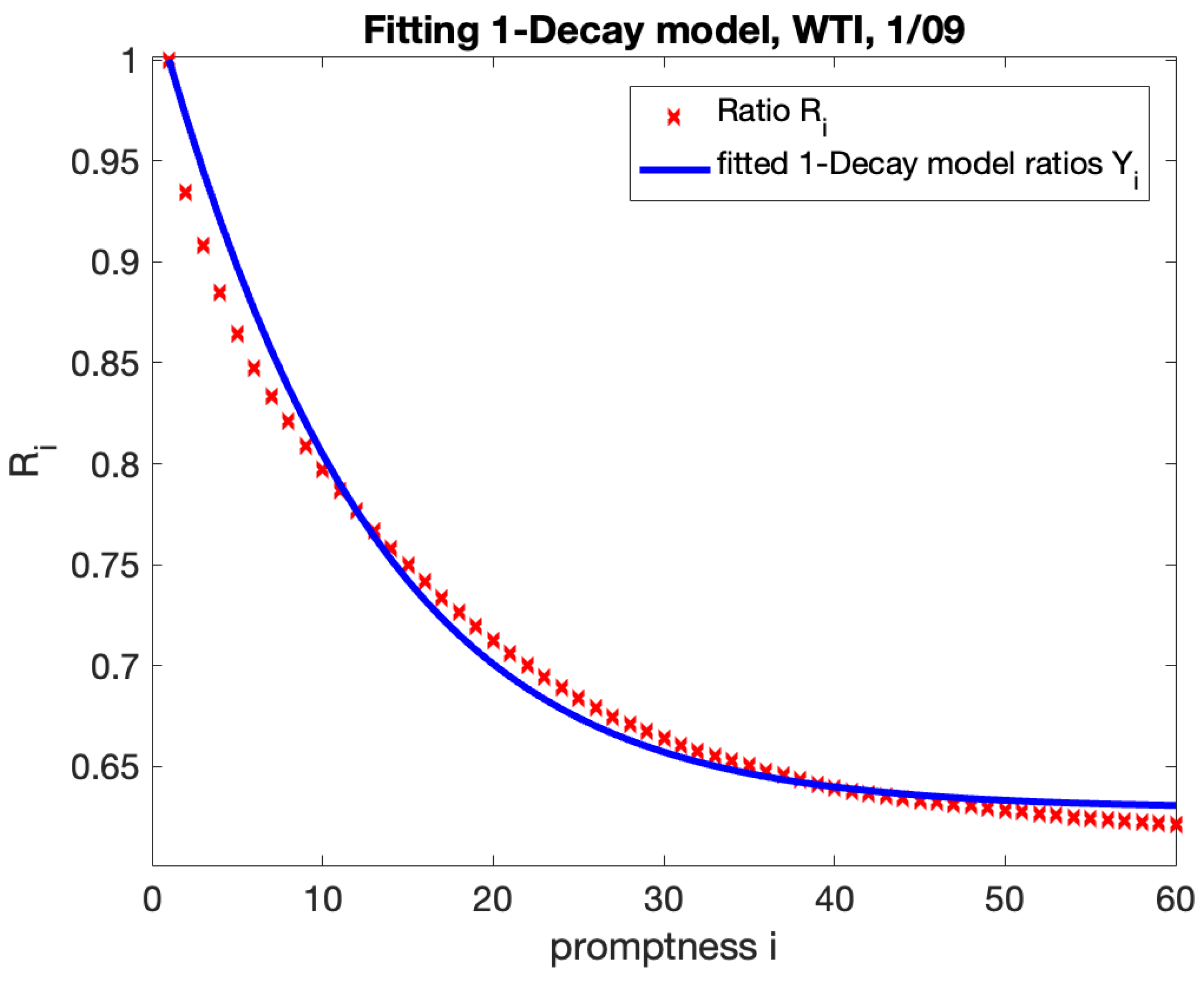
- The mean square error of the fit is .
- The estimates of correlations are presented on the plot:Figure A2. Correlations between the prompt and i-th nearby contract, computed using WTI log returns calculated on the period 12/19/2008 - 1/20/2009.Figure A2. Correlations between the prompt and i-th nearby contract, computed using WTI log returns calculated on the period 12/19/2008 - 1/20/2009.
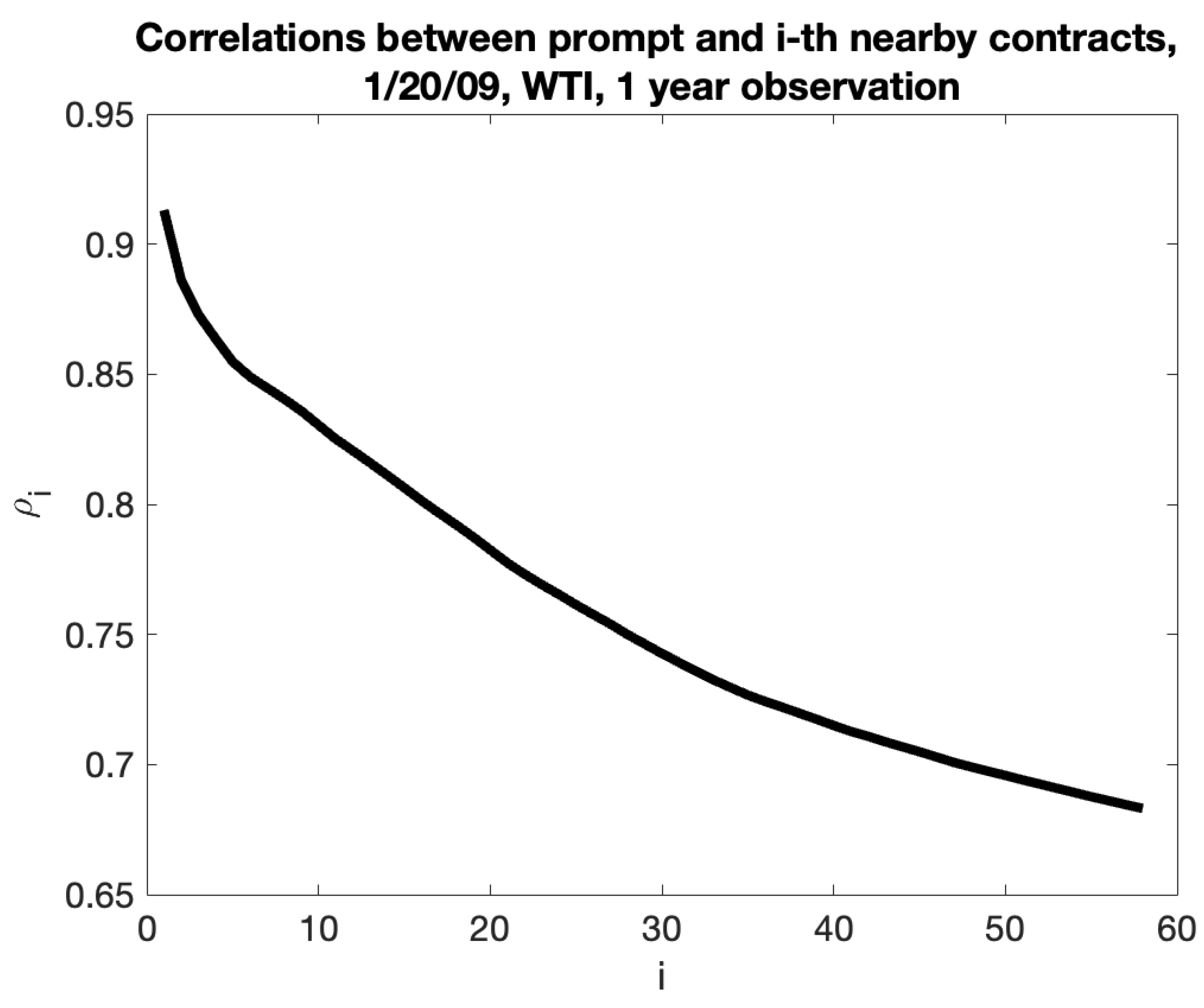
- The calculated lower bound of the statistical error (A5) is , thus the model fits well within the statistical error. Note that, we get practically the same lower bound, if instead of using the realized ratios , we use the model ratios with best fitted parameters.
-
Checking by Simulations We checked the formulas by simulations:
- Simulate daily prices of lognormal futures with known volatilities and correlations.
- For each simulation path, calculate the standard deviations of log-returns and the normalized ratios . Compute variance of across simulations.
- For each i, compare the variances of the ratios with the theoretical result (9). They are in good agreement, the average ratio real vs model, across simulations and contracts, is .
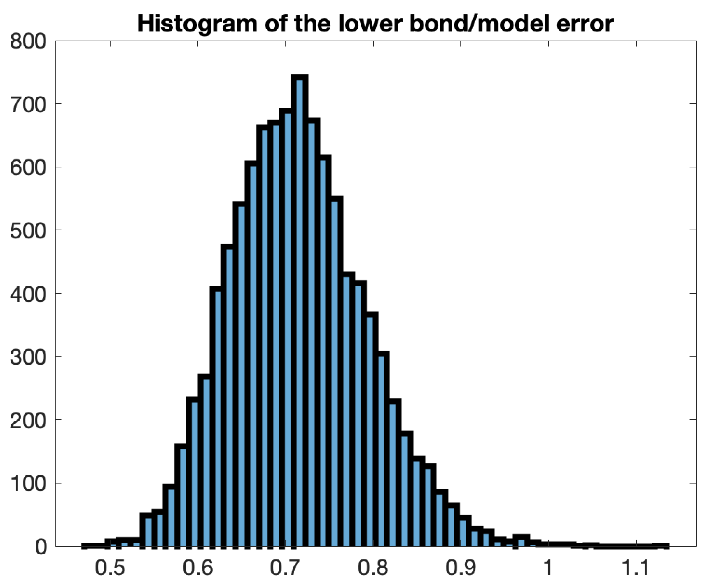
- For each i and each simulation path, compute the lower bound (A5) and compare vs the theoretical error. In average the lower bound is about of the model error. Figure A3 gives an example of the histogram of the ratios of the lower bound in each simulations divided by the model error. Only from all simulations give the value more than the model error.Figure A3. Checking by simulations, 10000 simulations paths, , , .
Appendix B. Cross Validation
Cross validation
Cross Validation (CV) is a technique used to get a more accurate estimate of out-of-sample accuracy. CV splits observations into two sets: the training set and the testing set. In the Samuelson case, the original dataset is given by volatilities of 60 nearby contracts. Following the standard CV process, we drop of data of the original dataset and keep the rest.
The volatility of prompt contract plays a crucial role in capturing Samuelson parameter B as it serves as a benchmark to normalize the volatilities of all other contracts. It also contributes the most to the increase in volatility as maturity approaches. For those reasons we choose to keep the return volatility of prompt contract and randomly drop 12 data points from the other 59 contracts. With the 48 data points, we repeat the calibration procedure and compare the fitted parameter, as well as in-sample and out-of-sample model errors obtained with the original data set. The procedure is as follows:
- Step 1: Generate 12 random numbers between 2 and 60 from uniform distribution, drop 12 data points from the data set. This is our testing set.
- Step 2: Perform the fitting procedure on the rest of data points (training set) , record the in-sample error and out-of-sample error.
- Step 3: Repeat step 1-3 for 100 times. Record out-of-sample errors and take averages of the 100 out-of-sample errors for all periods.
If the parameters estimated with training set are close to the original parameters, and the out-of-sample errors are reasonable, we can conclude that the model is stable.
In below table, we give statistics of cross validation procedure for WTI with different observation periods, such 2, 3... 12 months. Specifically, we report:
- The first column marked lists the average over all observation periods of the differences , where is the average of decay parameter B fitted on 100 randomized training sets; is the parameter B fitted on the whole set.
- Second column gives the maximum of the differences .
- In the third and the fourth column we similar statistics for the parameter .
- In the fifth column we report the average over all observation period of the differences between the out of sample errors and the in sample errors; and the last column gives the maximum of those differences.
In next table we report similar results of cross validation procedure for Brent.
Table A1.
WTI Cross Validation Results.
| 2m | 0.0010 | 0.0385 | 0.0003 | 0.0081 | 0.0021 | 0.0284 |
| 3m | 0.0009 | 0.0194 | 0.0003 | 0.0038 | 0.0022 | 0.0248 |
| 4m | 0.0008 | 0.0183 | 0.0002 | 0.0022 | 0.0022 | 0.0228 |
| 6m | 0.0008 | 0.0340 | 0.0002 | 0.0027 | 0.0023 | 0.0159 |
| 8m | 0.0006 | 0.0064 | 0.0002 | 0.0011 | 0.0024 | 0.0135 |
| 12m | 0.0009 | 0.0111 | 0.0002 | 0.0014 | 0.0026 | 0.0135 |
Table A2.
Brent Cross Validation Results.
| 2m | 0.0005 | 0.0107 | 0.0004 | 0.0096 | 0.0013 | 0.0168 |
| 3m | 0.0004 | 0.0065 | 0.0003 | 0.0054 | 0.0014 | 0.0156 |
| 4m | 0.0004 | 0.0040 | 0.0003 | 0.0028 | 0.0014 | 0.0134 |
| 6m | 0.0003 | 0.0044 | 0.0007 | 0.0526 | 0.0015 | 0.0102 |
| 8m | 0.0005 | 0.0082 | 0.0003 | 0.0101 | 0.0016 | 0.0092 |
| 12m | 0.0003 | 0.0021 | 0.0003 | 0.0055 | 0.0017 | 0.0079 |
Table A3.
WTI Cross Validation Results.
| Max. B diff | Mean. - | Max. - | Mean. - RMSE | Max. - RMSE | |
|---|---|---|---|---|---|
| 2m | 0.0385 | 0.0021 | 0.0284 | 0.0025 | 0.0136 |
| 3m | 0.0194 | 0.0022 | 0.0248 | 0.0024 | 0.0081 |
| 4m | 0.0183 | 0.0022 | 0.0228 | 0.0024 | 0.0134 |
| 6m | 0.0340 | 0.0023 | 0.0159 | 0.0026 | 0.0158 |
| 8m | 0.0064 | 0.0024 | 0.0135 | 0.0028 | 0.0156 |
| 12m | 0.0111 | 0.0026 | 0.0135 | 0.0033 | 0.0183 |
The results illustrates the stability of the fitted parameters, thus stability of the model.
References
- Samuelson, P. Proof that Properly Anticipated Prices Fluctuate Randomly. Industrial Management Review 1965, 6, 41–49. [Google Scholar]
- Galeeva, R.; Haversang, T. Parameterized Calendar Correlations: Decoding Oil and Beyond. The Journal of Derivatives 2020, 27, 7–25. [Google Scholar] [CrossRef]
- Miller, K. The Relation between Volatility and Maturity in Futures Contracts. Chicago Mercantile Exchange 1979, 25–36. [Google Scholar]
- Barnhill, T.M.; Jordan, J.; Seale, W. Maturity and refunding effects on Treasury bond futures price variance. Journal of Financial Research 1987, 1987 10, 121–131. [Google Scholar] [CrossRef]
- Adrangi, B.; Chatrath, A.; Dhanda, K.; Raffiee, K. Chaos in oil prices? Evidence from futures markets. Energy Economics 2001, 23, 405–425. [Google Scholar] [CrossRef]
- Adrangi, B.; Chatrath, A.; Dhanda, K.; Raffiee, K. on-linear dynamics in futures prices: Evidence from Coffee, Sugar and Cocoa Exchange. Applied Financial Economics 2003, 13, 245–256. [Google Scholar] [CrossRef]
- Andersen, R. Some determinants of the volatility of futures prices. The Journal of Futures Markets, 1985, 5. [Google Scholar] [CrossRef]
- Milonas, N. Price Variability and the Maturity Effect in Futures Markets. Futures Markets 1986, 3, 443–460. [Google Scholar] [CrossRef]
- Rutledge, D. A note on the variability of futures prices. Review of Economics and Statistics 1976, 58, 118–120. [Google Scholar] [CrossRef]
- Galloway, T.; Kolb, R. Futures prices and the maturity effect. Journal of Futures Markets, 1996, 16, 809–828. [Google Scholar] [CrossRef]
- Liu, W. (2021). Revisiting the Samuelson hypothesis on energy futures. Quantitative Finance 2021, 12, n12. [Google Scholar]
- Jaeck, E.; Lautier, D. Volatility in electricity derivative markets: The Samuelson effect revisited. Energy Economics 2016, 59, 300–313. [Google Scholar] [CrossRef]
- Grammatikos, T.; Sauders, A. Futures Price Variability: A Test of Maturity and Volume Effects. The Journal of Business. [CrossRef]
- Park, H.; Sears, R. Estimating stock index futures volatility through the price of their options. Journal of Futures Markets, 1985, 5, 123–138. [Google Scholar] [CrossRef]
- Bessembinder, H.; Coughenour, J.; Sequin, P.; Smeller, M. Is There a Term Structure of Futures Volatilities? Journal of Derivatives 1996, 4(2), 45–58. [Google Scholar] [CrossRef]
- Brooks, R. Samuelson hypothesis and carry arbitrage. Journal of Derivatives 2012, 20(2), 37–65. [Google Scholar] [CrossRef]
- Brooks, R.; Teterin, P. Samuelson hypothesis, arbitrage activity, and futures term premiums. Journal of Future Markets 1441. [Google Scholar] [CrossRef]
- Nelson, C.; Siegel, A. Parsimonious Modeling of Yield Curves/. The Journal of Biseness 1982, 60, 473–489. [Google Scholar] [CrossRef]
- Clewlow L, Strickland Ch. Energy Derivatives: Pricing and Risk Management Lacima Publications 2020.
- Schwartz, E. The Stochastic Behavior of Commodity Prices: Implications for Valuation and Hedging. Journal of Finance 1997, 52, n3–923. [Google Scholar] [CrossRef]
- Gibson, R.; Schwartz, E. Stochastic Convenience Yield and the Pricing of Oil Contingent Claims. Journal of Finance 1990, 45, 959–976. [Google Scholar] [CrossRef]
- Pilipović D. Energy Risk: Valuing and Managing Energy Derivatives McGraw-Hill 1987.
- Trolle, A. , Schwartz E. Unspanned stochastic volatility and the pricing of commodity derivatives. Review of Financial Studies 2009, 22(11), 4423–4461. [Google Scholar] [CrossRef]
- Crosby, J.; Frau, C. Jumps in commodity prices: New approaches for pricing plain vanilla options. Energy Economics 2022, 114. [Google Scholar] [CrossRef]
- Frau, C.; Fanelli, V. Seasonality in commodity prices: New approaches for pricing plain vanilla options. Annals of Operations Research 2023, 336, 1089–1131. [Google Scholar] [CrossRef]
- Hilliard, J.; Hilliard, J. A jump-diffusion model for pricing and hedging with margined options: An application to Brent crude oil contracts. Journal of Banking and Finance 2019, 98, 137–155. [Google Scholar] [CrossRef]
- Chiarella, C.; Kang, C. Sklibosios Nikitopoulos Ch., and Thuy-Duong T. Humps in the volatility structure of the crude oil futures market: New evidence. Energy Economics 2013, 40, 989–1000. [Google Scholar] [CrossRef]
- Schneider, L.; Tavin, B. From the Samuelson volatility effect to a Samuelson correlation effect: An analysis of crude oil calendar spread options. Journal of Banking & Finance 2018, 95, 185–202. [Google Scholar]
- Swindle G. Valuation and Risk Management in Energy Markets. Cambridge books 2014.
- Joarder, A. Moments of the product and ratio of two correlated chi-square variables. Stat. Papers, Open Access 2009, 50, 581–592. [Google Scholar] [CrossRef]
- Li, Y.; Wang, W. Snowball structure pricing and risk in-depth analysis. Advances in Economics, Business and Management Research 2022, 211. [Google Scholar]
| 1 | In industry such contracts are called constant maturity contracts, and used for risk management purposes |
| 2 | Brooks and Teterin [17] called it "the maturity drift problem" |
| 3 | For example, Ercot futures expire pm the second to last business day of the month prior to the contract month |
| 4 | Specifically, we must utilize the expiration of the option on the future . For the sake of simplicity, we elect to disregard this difference and assume
|
| 5 | A very close result can be obtained by using quantiles of the chi-square distribution, with confidence level of
|
Figure 1.
Illustration of concept of Samuelson Time.
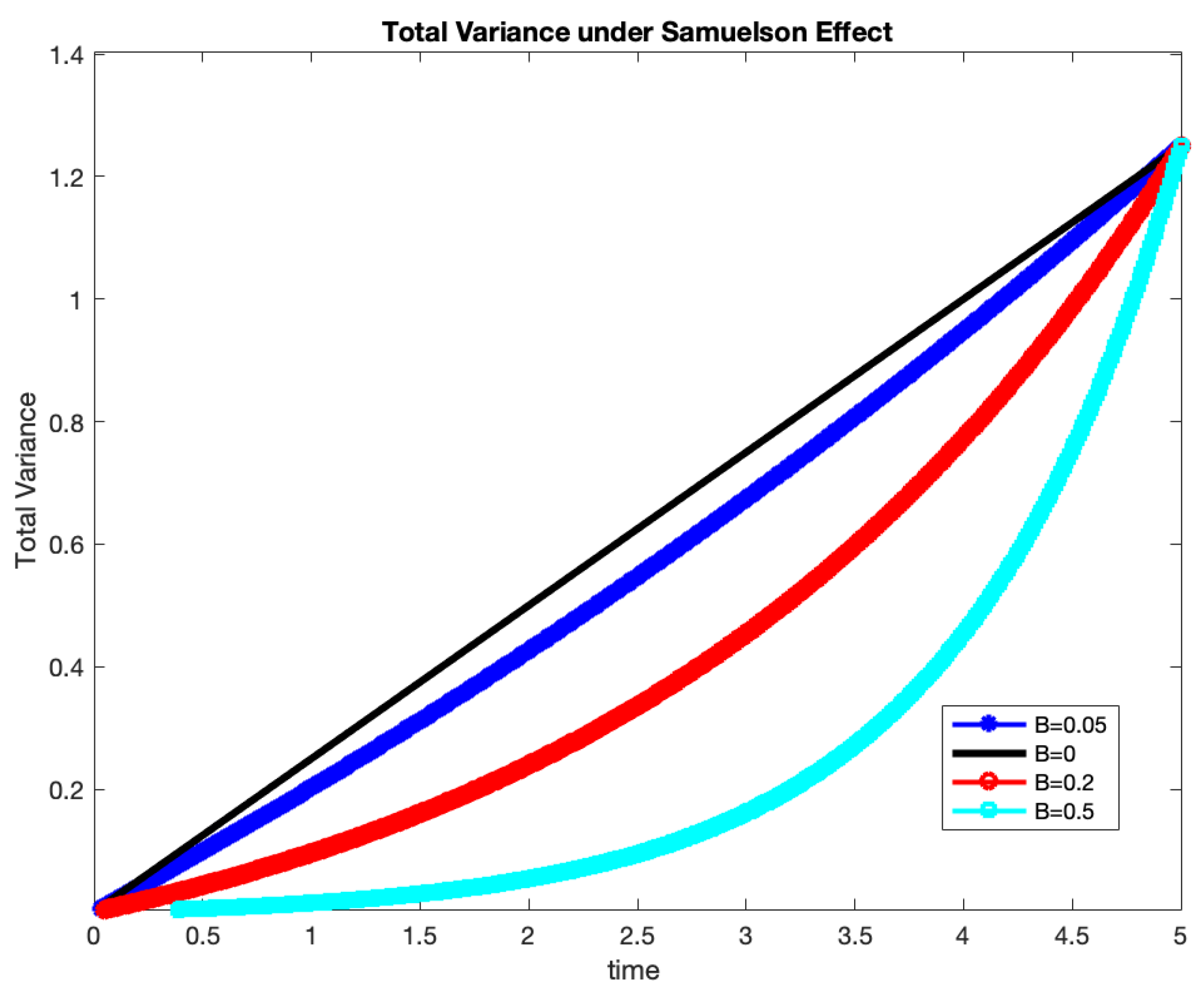
Figure 2.
Implied Volatility of WTI futures as November 2018 (source: Bloomberg), and realized Volatilities of WTI nearby futures, calculated on 2 months, September and October 2018.
Figure 2.
Implied Volatility of WTI futures as November 2018 (source: Bloomberg), and realized Volatilities of WTI nearby futures, calculated on 2 months, September and October 2018.
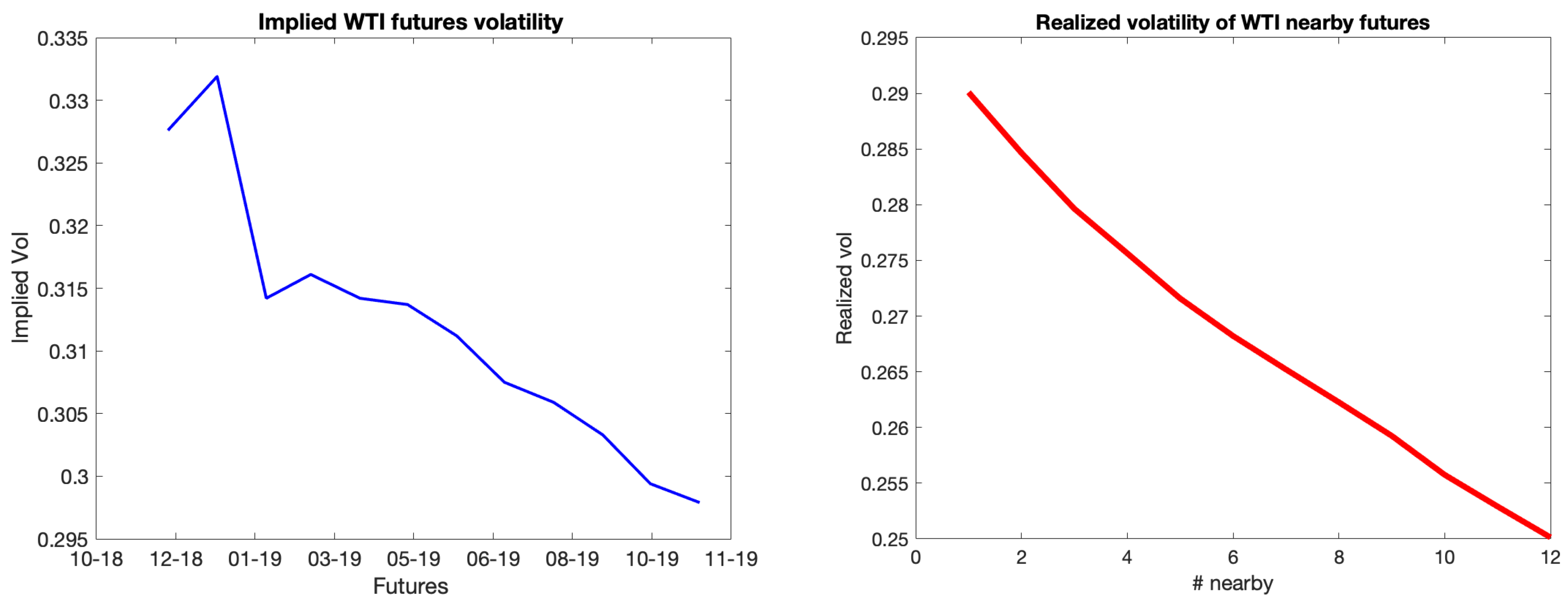
Figure 3.
Contour Plots of the ratio for Decay Model.
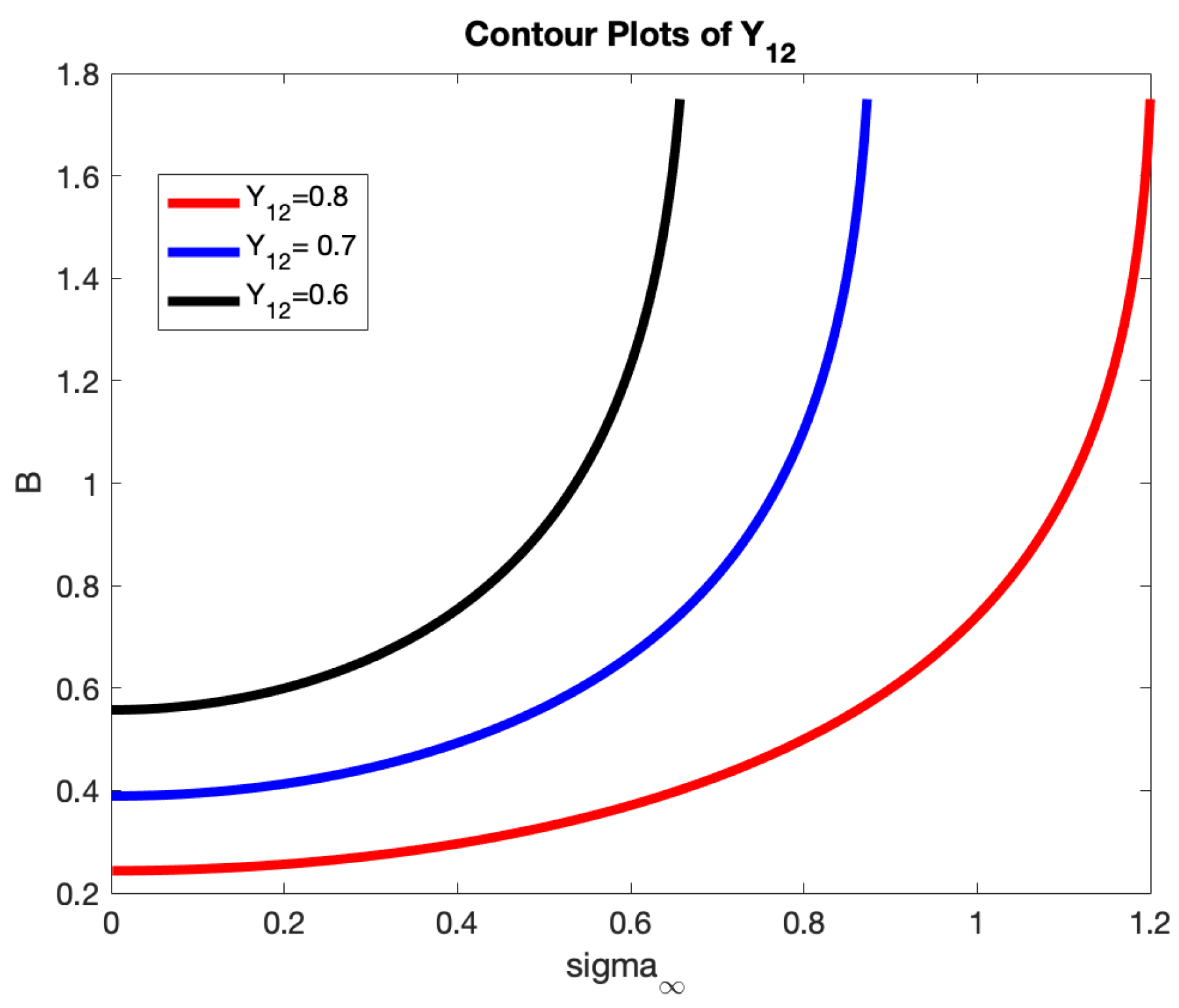
Figure 4.
US Monthly Supply & Demand data
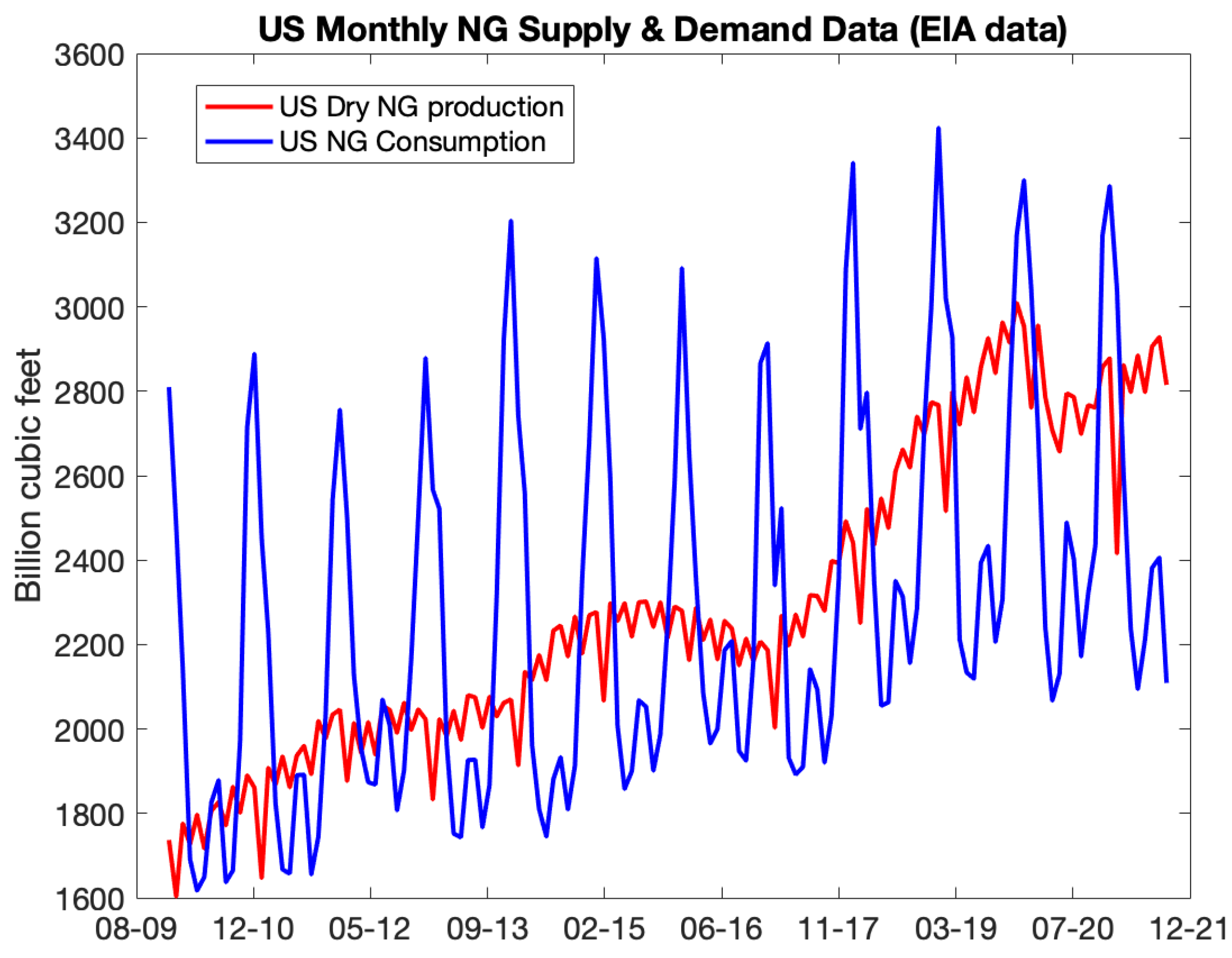
Figure 5.
Implied NG Volatility in June 2020, source: Bloomberg data
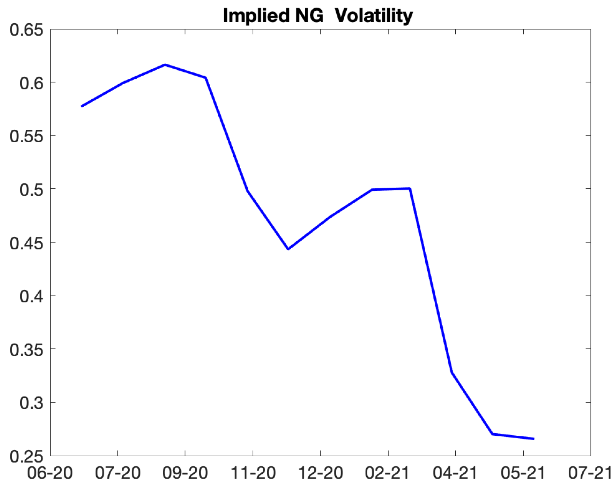
Figure 6.
This graph illustrates the actual WTI volatility compared to the fitted volatility generated from the 1-decay model. The realized volatility has been calculated using WTI log returns from 02/21/2019 to 02/20/2020.
Figure 6.
This graph illustrates the actual WTI volatility compared to the fitted volatility generated from the 1-decay model. The realized volatility has been calculated using WTI log returns from 02/21/2019 to 02/20/2020.
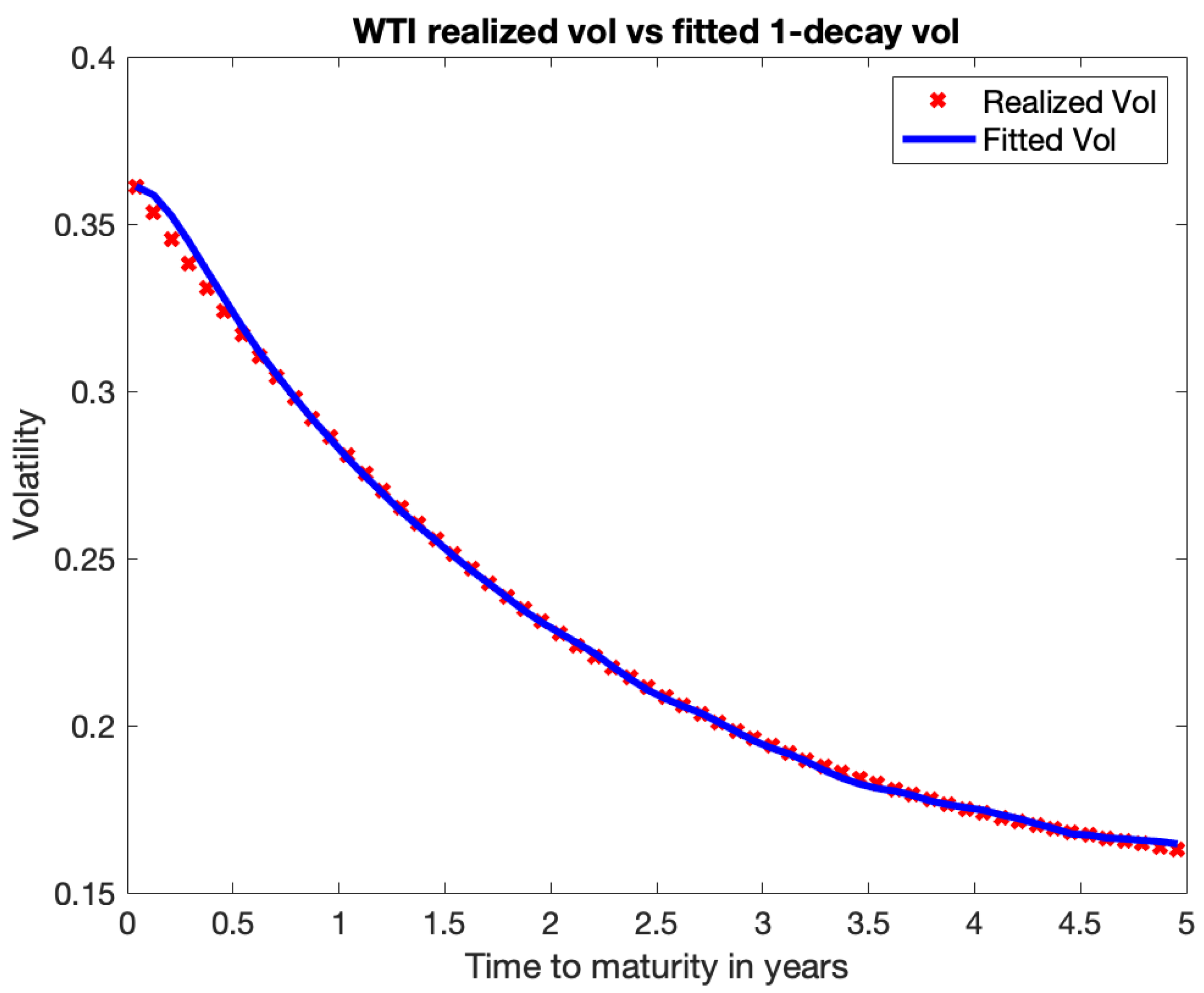
Figure 7.
This graph illustrates the actual NG volatility compared to the fitted volatility with a 1-decay model. The realized volatility is calculated using the log returns of Natural Gas for the period from October 30, 2019, to December 27, 2019.
Figure 7.
This graph illustrates the actual NG volatility compared to the fitted volatility with a 1-decay model. The realized volatility is calculated using the log returns of Natural Gas for the period from October 30, 2019, to December 27, 2019.
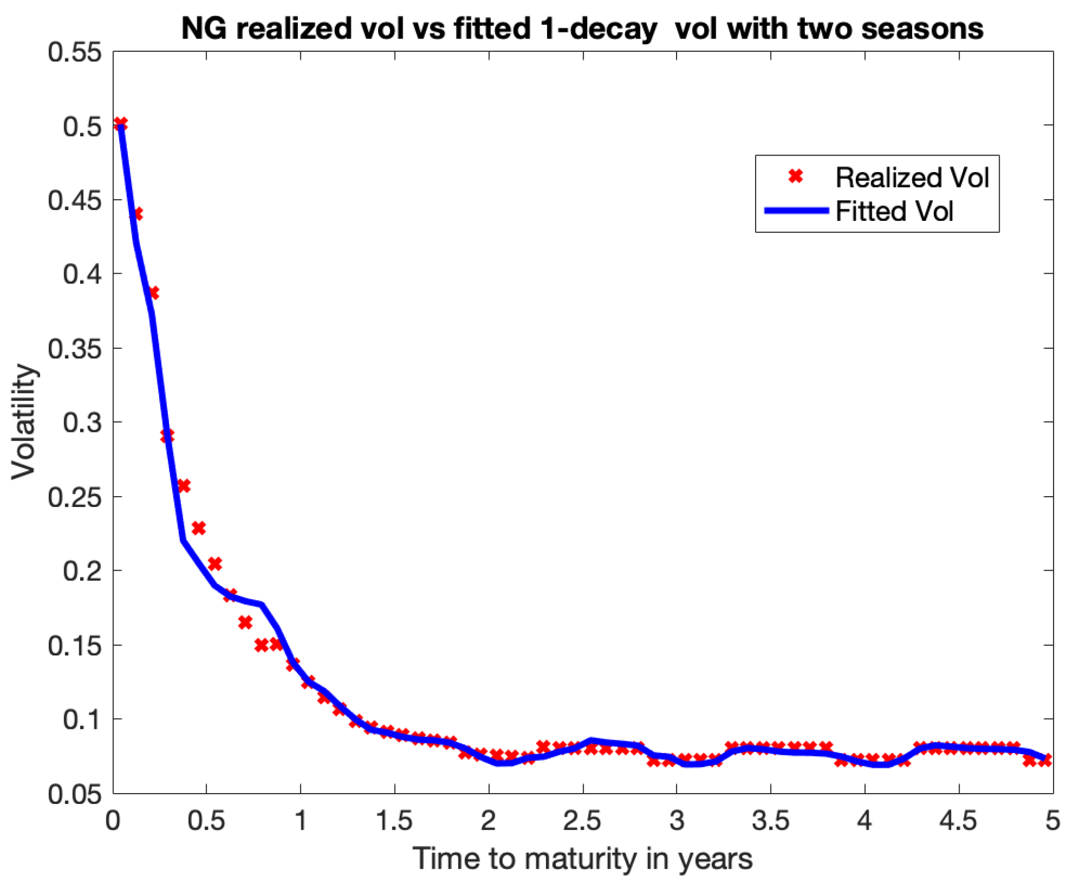
Figure 10.
The graph illustrates the actual WTI instantaneous volatility compared to the fitted volatility calculated using both the 1-decay and 2-decay models. The realized volatility is calculated using WTI log returns from the period of November 21, 2008, to November 20, 2009.
Figure 10.
The graph illustrates the actual WTI instantaneous volatility compared to the fitted volatility calculated using both the 1-decay and 2-decay models. The realized volatility is calculated using WTI log returns from the period of November 21, 2008, to November 20, 2009.
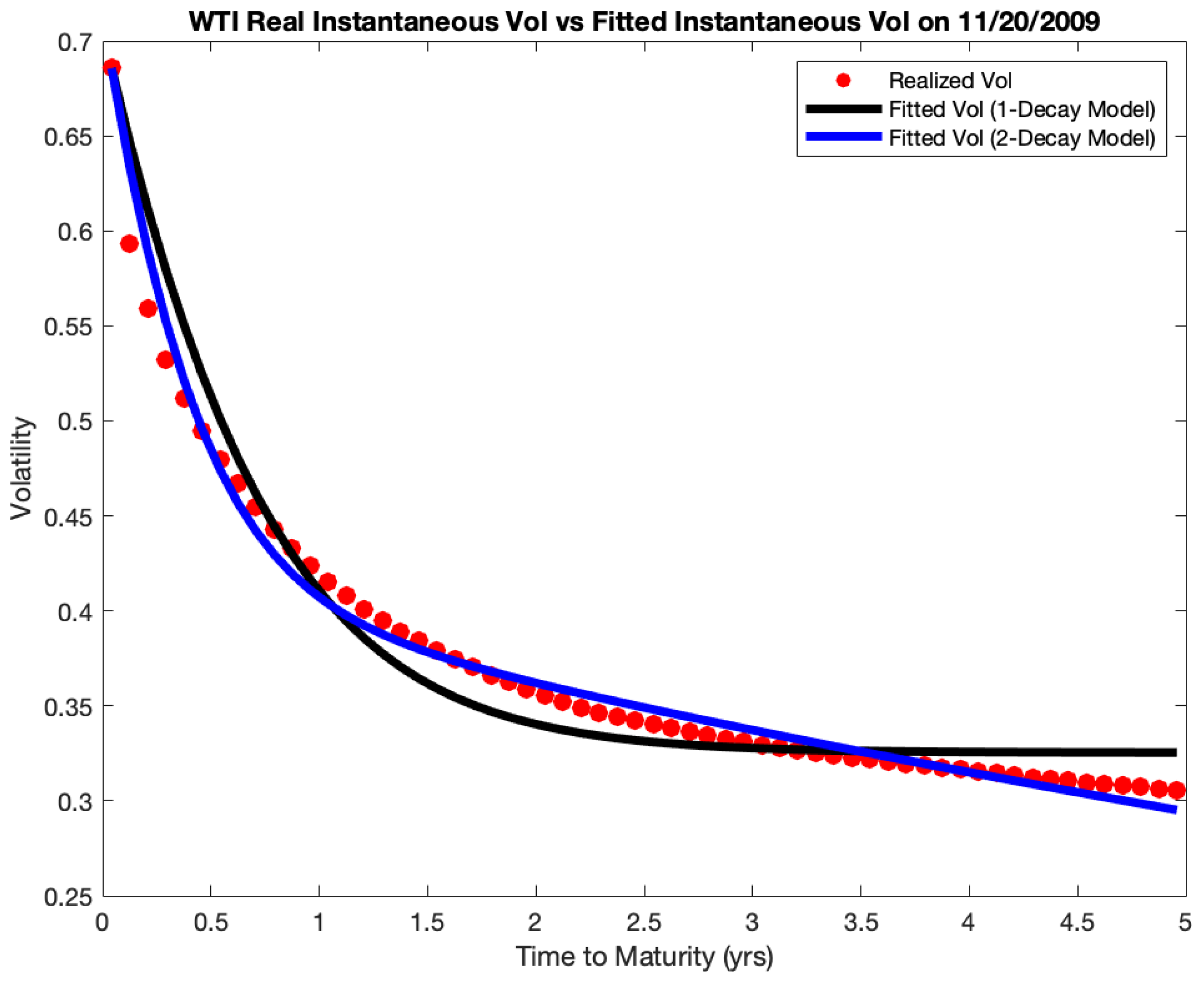
Figure 11.
ATM Peak Monthly and Daily Volatilities as of January 5 2023, ERCOT North, published by Argus Media.
Figure 11.
ATM Peak Monthly and Daily Volatilities as of January 5 2023, ERCOT North, published by Argus Media.
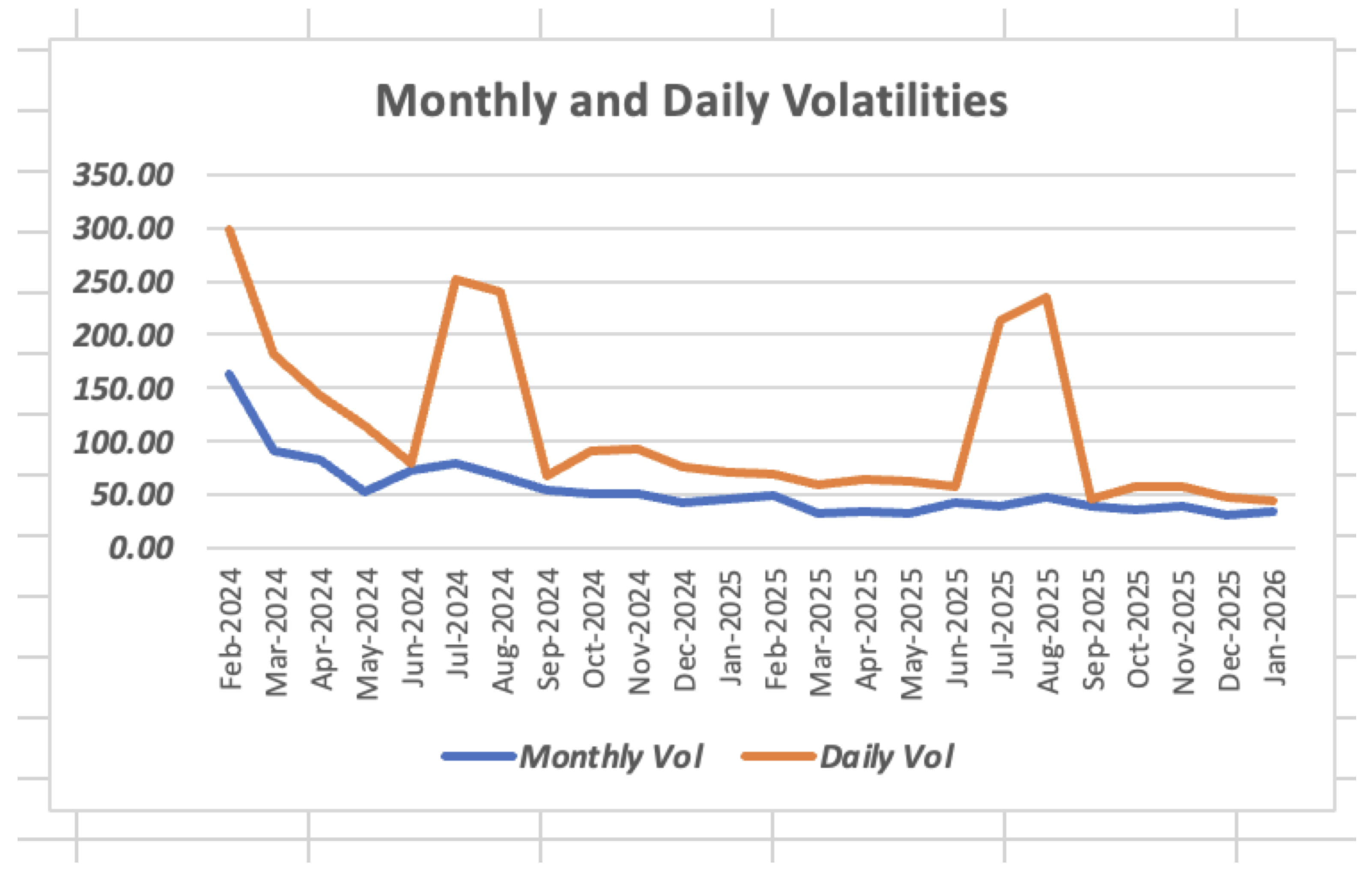
Figure 12.
Comparison of histograms by historical simulation vs Monte Carlo.
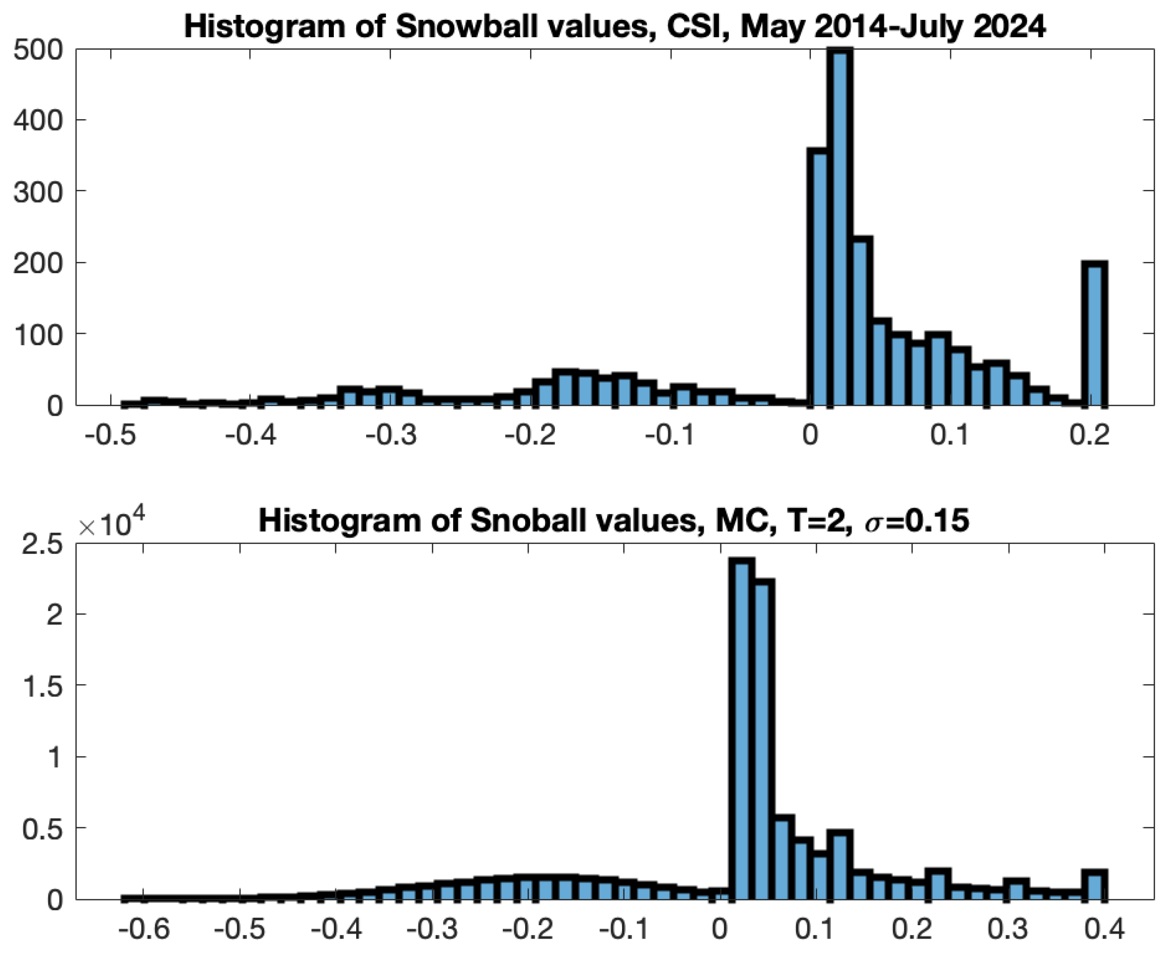
Figure 13.
The normalized index CSI 500 price history 9/22- 9/23 with the best snowball payoff
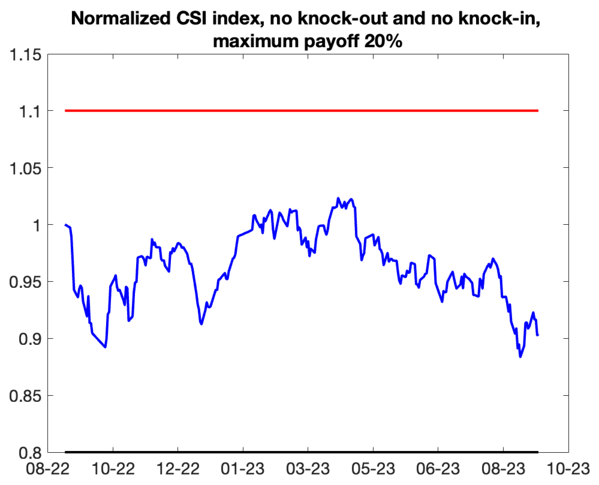
Figure 14.
The normalized index CSI 500 price history 5/15- 5/16with the worst snowball payoff
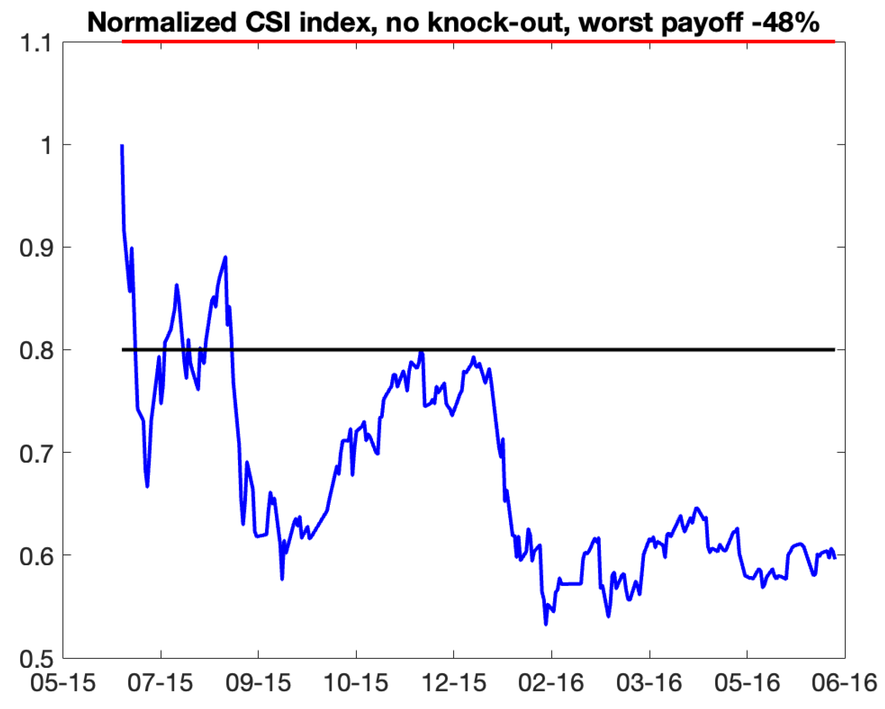
Figure 15.
The expected snowball payoff vs volatility of the underlying
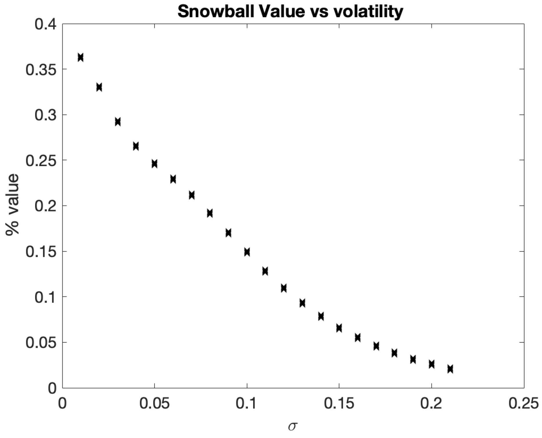
Figure 16.
The expected snowball payoff for different decay values B, ,
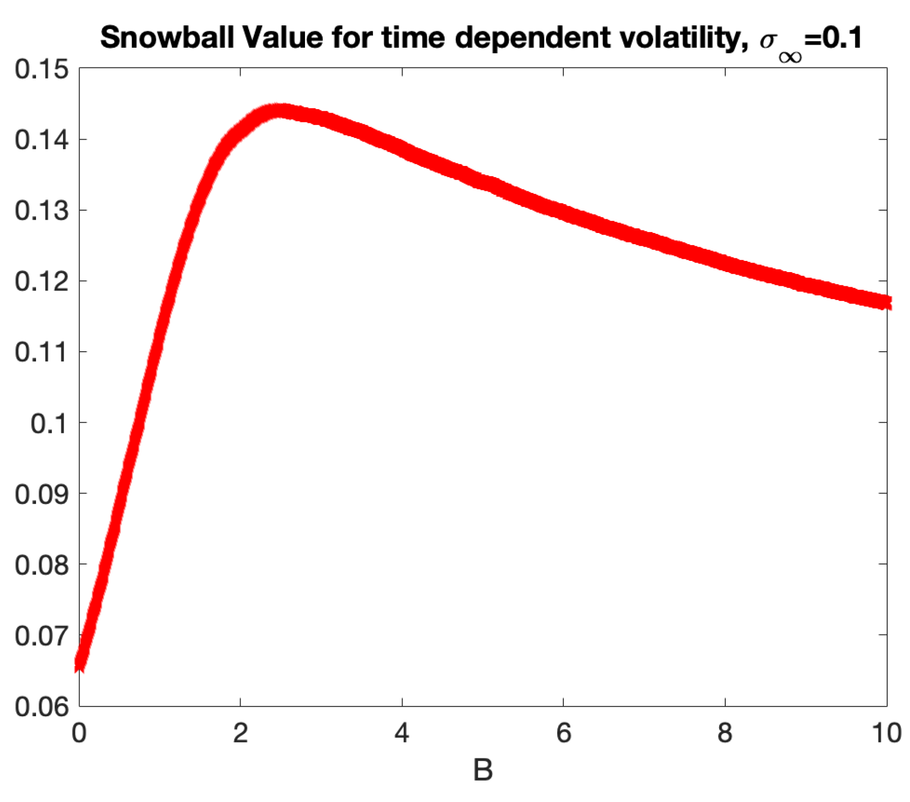
Table 1.
Descriptive statistics of WTI, Brent and Natural Gas return series.
| Series | Count | Mean | Std. Dev. | Median | Minimum | Maximum | Skewness | Kurtosis |
|---|---|---|---|---|---|---|---|---|
| Data 1: WTI (Data Period: 04/21/2006 - 06/09/2021) | ||||||||
| WTI1 | 3813 | |||||||
| WTI2 | 3813 | |||||||
| WTI3 | 3813 | |||||||
| WTI4 | 3813 | |||||||
| Data 2: Brent (Data Period: 06/16/2006 - 06/09/2021) | ||||||||
| Brent1 | 3869 | |||||||
| Brent2 | 3869 | |||||||
| Brent3 | 3869 | |||||||
| Brent4 | 3869 | |||||||
| Data 3: Natural Gas (Data Period: 06/29/2006 - 06/09/2021) | ||||||||
| NG1 | 3772 | |||||||
| NG2 | 3772 | |||||||
| NG3 | 3772 | |||||||
| NG4 | 3772 | |||||||
Table 2.
WTI Calibration Result Examples.
| B | RMSE | |||
|---|---|---|---|---|
| 12/21/11 | 12/19/12 | 0.2937 | 0.5678 | 0.0014 |
| 11/19/12 | 11/20/13 | 0.4611 | 0.4953 | 0.0003 |
| 10/23/13 | 10/21/14 | 0.6627 | 0.4663 | 0.0004 |
| 9/23/14 | 9/22/15 | 0.4803 | 0.4856 | 0.0006 |
| 8/21/15 | 8/22/16 | 0.4624 | 0.5773 | 0.0063 |
| 7/21/16 | 7/20/17 | 0.3959 | 0.5966 | 0.0007 |
| 6/21/17 | 6/20/18 | 0.4864 | 0.6964 | 0.0008 |
| 5/23/18 | 5/21/19 | 0.2980 | 0.6775 | 0.0008 |
| 4/23/19 | 4/21/20 | 0.9093 | 0.3028 | 0.0252 |
| 02/21/19 | 02/20/20 | 0.3245 | 0.4458 | 0.0018 |
Table 3.
Examples of Brent Calibration Results Utilizing the 1-Decay Mode.l
| B | RMSE | |||
|---|---|---|---|---|
| 10/17/12 | 10/16/13 | 0.2809 | 0.4159 | 0.0013 |
| 9/16/13 | 9/15/14 | 0.5306 | 0.4917 | 0.0004 |
| 8/15/14 | 8/14/15 | 0.3821 | 0.4267 | 0.0026 |
| 8/17/15 | 7/29/16 | 0.3498 | 0.5520 | 0.0012 |
| 7/1/16 | 6/30/17 | 0.3367 | 0.5495 | 0.00175 |
| 6/1/17 | 5/31/18 | 0.3629 | 0.6853 | 0.0025 |
| 5/1/18 | 4/30/19 | 0.2325 | 0.5715 | 0.0006 |
| 4/1/19 | 3/31/20 | 0.4789 | 0.3813 | 0.005 |
Table 4.
Natural Gas Calibration Results; "W" denotes winter, whereas "S" signifies summer.
| B W | W | B S | S | RMSE | |
|---|---|---|---|---|---|
Disclaimer/Publisher’s Note: The statements, opinions and data contained in all publications are solely those of the individual author(s) and contributor(s) and not of MDPI and/or the editor(s). MDPI and/or the editor(s) disclaim responsibility for any injury to people or property resulting from any ideas, methods, instructions or products referred to in the content. |
© 2025 by the authors. Licensee MDPI, Basel, Switzerland. This article is an open access article distributed under the terms and conditions of the Creative Commons Attribution (CC BY) license (http://creativecommons.org/licenses/by/4.0/).
Copyright: This open access article is published under a Creative Commons CC BY 4.0 license, which permit the free download, distribution, and reuse, provided that the author and preprint are cited in any reuse.


